Earth System Model Evaluation Tool (ESMValTool) v2.0 - diagnostics for emergent constraints and future projections from Earth system models in ...
←
→
Page content transcription
If your browser does not render page correctly, please read the page content below
Geosci. Model Dev., 13, 4205–4228, 2020
https://doi.org/10.5194/gmd-13-4205-2020
© Author(s) 2020. This work is distributed under
the Creative Commons Attribution 4.0 License.

Earth System Model Evaluation Tool (ESMValTool) v2.0 –
diagnostics for emergent constraints and future projections from
Earth system models in CMIP
Axel Lauer1 , Veronika Eyring1,2 , Omar Bellprat3 , Lisa Bock1 , Bettina K. Gier2,1 , Alasdair Hunter5 , Ruth Lorenz4 ,
Núria Pérez-Zanón5 , Mattia Righi1 , Manuel Schlund1 , Daniel Senftleben1 , Katja Weigel2,1 , and Sabrina Zechlau1
1 Deutsches Zentrum für Luft- und Raumfahrt (DLR), Institut für Physik der Atmosphäre, Oberpfaffenhofen, Germany
2 Universityof Bremen, Institute of Environmental Physics (IUP), Bremen, Germany
3 Swiss Federal Department of Foreign Affairs, Bern, Switzerland
4 ETH Zurich, Institute for Atmospheric and Climate Science, Zurich, Switzerland
5 Barcelona Supercomputing Center (BSC), Barcelona, Spain

Correspondence: Axel Lauer (axel.lauer@dlr.de)

Received: 26 February 2020 – Discussion started: 18 March 2020
Revised: 26 June 2020 – Accepted: 20 July 2020 – Published: 10 September 2020

Abstract. The Earth System Model Evaluation Tool (ES-            Intergovernmental Panel on Climate Change’s (IPCC) Fifth
MValTool), a community diagnostics and performance met-          Assessment Report (AR5) and various multi-model statistics.
rics tool for evaluation and analysis of Earth system mod-
els (ESMs), is designed to facilitate a more comprehensive
and rapid comparison of single or multiple models participat-
ing in the Coupled Model Intercomparison Project (CMIP).         1   Introduction
The ESM results can be compared against observations or re-
analysis data as well as against other models including pre-     Climate models are important tools not only to improve our
decessor versions of the same model. The updated and ex-         understanding of the key processes in present-day climate but
tended version (v2.0) of the ESMValTool includes several         also to project future climate change under different plausi-
new analysis scripts such as large-scale diagnostics for eval-   ble scenarios. Climate models have been continuously im-
uation of ESMs as well as diagnostics for extreme events, re-    proved and extended over the last decades from relatively
gional model and impact evaluation. In this paper, the newly     simple atmosphere-only models to the complex state-of-the-
implemented climate metrics such as effective climate sensi-     art Earth system models (ESMs) participating in the latest
tivity (ECS) and transient climate response (TCR) as well        (sixth) phase of the Coupled Model Intercomparison Project
as emergent constraints for various climate-relevant feed-       (CMIP6; Eyring et al., 2016a). The increasing complexity of
backs and diagnostics for future projections from ESMs are       the models is needed to represent key feedbacks that affect
described and illustrated with examples using results from       climate change but is also likely to increase the spread of cli-
the well-established model ensemble CMIP5. The emergent          mate projections across the multi-model ensemble (Eyring et
constraints implemented include constraints on ECS, snow-        al., 2019). This poses a challenge for evaluation and analysis
albedo effect, climate–carbon cycle feedback, hydrologic cy-     of the model results that requires efficient tools able to han-
cle intensification, future Indian summer monsoon precipi-       dle the increasing number of variables, processes and also the
tation and year of disappearance of summer Arctic sea ice.       increasing data volume.
The diagnostics included in ESMValTool v2.0 to analyze fu-          The Earth System Model Evaluation Tool (ESMValTool),
ture climate projections from ESMs further include analy-        released in a first version in 2016 (Eyring et al., 2016b),
sis scripts to reproduce selected figures of chapter 12 of the   has been developed with the aim of taking model evalua-
                                                                 tion to the next level by facilitating analysis of many dif-

Published by Copernicus Publications on behalf of the European Geosciences Union.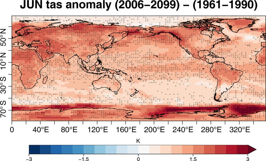
4206                                                A. Lauer et al.: Earth System Model Evaluation Tool (ESMValTool) v2.0

ferent ESM components, providing well-documented source             al. (2013). Furthermore, diagnostics tailored to analyze pro-
code and scientific background of implemented diagnostics           jections of sea ice such as calculation of the year of disap-
and metrics and allowing for traceability and reproducibil-         pearance (sea ice extent below 1 million km2 ) from a multi-
ity of results (provenance). This has been made possible by         model ensemble and to constrain the future austral jet posi-
a lively and growing development community continuously             tion have been added. A newly implemented “toy model” can
improving the tool supported by multiple national and Eu-           be used to generate synthetic members of a single dataset.
ropean projects. Version 2.0 (v2.0) of the ESMValTool has           When providing an estimate for the standard error of ob-
been developed as a large community effort to specifically          servations, e.g., from differences between different observa-
target the increased data volume of CMIP6 and the related           tional datasets, this toy model can be used to investigate and
challenges posed by analysis and evaluation of output from          take into account the effect of observational uncertainty in
multiple high-resolution and complex ESMs.                          model evaluation (Sect. 3.4). A summary is given in Sect. 4.
   For this, the core functionalities have been completely          The aim of this paper is to document and illustrate how these
rewritten in order to take advantage of state-of-the-art com-       newly added ESMValTool “recipes”, i.e., configuration files
putational libraries and methods to allow for faster, more ef-      defining input, preprocessing, diagnostics and run-time op-
ficient and user-friendly data processing (Righi et al., 2020).     tions of the ESMValTool, can be used for model evaluation
Besides many technical improvements, ESMValTool v2.0 in-            and analysis.
cludes new large-scale diagnostics for evaluation of Earth
system models (Eyring et al., 2020) and diagnostics for ex-
treme events, regional model and impact evaluation and anal-        2   Models and observations
ysis of ESM results (Weigel et al., 2020). As part of a series
of four articles describing the new features and diagnostics        The open-source release of ESMValTool (v2.0) that accom-
of the Earth System Model Evaluation Tool v2.0, this paper          panies this paper is intended to work with CMIP5 and
focuses on the newly included diagnostics for emergent con-         CMIP6 model output (and partly also with CMIP3 if the re-
straints and for analysis of future projections from ESMs as        quired output has been generated), but the tool is compatible
well as multi-model products (Sect. 3.1) and the two new            with any arbitrary model output, provided that it is in CF-
climate metrics: effective climate sensitivity (ECS) and tran-      compliant (CF: Climate and Forecast; http://cfconventions.
sient climate response (TCR) (Sect. 3.2).                           org/, last access: 18 June 2020) NetCDF format and
   An emergent constraint is a relationship across an ensem-        that the variables and metadata are following the CMOR
ble of models between some aspect of the Earth system sen-          (Climate Model Output Rewriter; https://pcmdi.github.
sitivity and an observable trend or variation in the current cli-   io/cmor-site/media/pdf/cmor_users_guide.pdf, last access:
mate, which offers the possibility to reduce uncertainties in       18 June 2020) tables and definitions (e.g., https://github.
climate projections. Furthermore, emergent constraints can          com/PCMDI/cmip6-cmor-tables/tree/master/Tables, last ac-
help guide model development onto processes crucial to the          cess: 7 November 2019, for CMIP6). These tables read in
magnitude and spread of future climate change projections           by the ESMValTool contain the definition of all variables,
and to point out future observational priorities (Eyring et al.,    together with their metadata such as units and standard and
2019). Emergent constraints implemented in ESMValTool               long names. Observations used in the evaluation are detailed
v2.0 (Sect. 3.3) include seven different approaches to con-         in the various sections of the paper (see also Sect. 6) and sum-
strain ECS as well as constraints for the hydrological cycle        marized in Tables 1 and 2 but should also be seen as examples
intensification, snow-albedo effect, year of disappearance of       as they can be easily replaced by other observational datasets
summer Arctic sea ice, future Indian summer monsoon pre-            provided they follow the CMOR convention. For selected ob-
cipitation and climate–carbon cycle feedback.                       servational datasets, CMORizing scripts are provided with
   For the analysis of ESM projections, ESMValTool v2.0             the ESMValTool that contain detailed downloading and pro-
now includes diagnostics to reproduce selected figures from         cessing instructions to convert the datasets into a CMOR-like
chapter 12 (Long-term Climate Change: Projections, Com-             format that can be processed by the ESMValTool. These re-
mitments and Irreversibility) of the IPCC AR5 (Collins et           format scripts serve as examples for writing similar scripts
al., 2013). These include figures showing the change in a           for other observational datasets that do not follow the CMOR
variable between historical and future periods, e.g., maps          standard. Such other datasets that are not available via
(2-D variables), zonal means (3-D variables), time series           the obs4mips (https://esgf-node.llnl.gov/projects/obs4mips/,
showing the change in certain variables from historical to          last access: 26 February 2020) or ana4mips (https://esgf.
future periods for multiple scenarios and maps visualizing          nccs.nasa.gov/projects/ana4mips/, last access: 30 June 2019)
change in variables normalized by global mean tempera-              projects and for which no CMORizing scripts are provided
ture change (pattern scaling) and the possibility to show sta-      can be used with the ESMValTool in two ways. The first is
tistical significance of changes when compared to natural           to write a new CMORizing script using an available one as
variability and the degree of agreement between the mod-            a template to generate a local copy of CMORized data that
els using the stippling and hatching methods as in Collins et       can readily be used with the ESMValTool. This typically in-

Geosci. Model Dev., 13, 4205–4228, 2020                                             https://doi.org/10.5194/gmd-13-4205-2020
A. Lauer et al.: Earth System Model Evaluation Tool (ESMValTool) v2.0                                                                                        4207

Table 1. Overview of recipes for emergent constraints and future projections implemented in ESMValTool (v2.0) along with the section
where they are described, a brief description, the required CMIP5 variables, the diagnostic scripts included and the observational datasets
used in the examples. All diagnostics expect time series of monthly mean data as input. For further technical details, we refer to the GitHub
repository.

 Recipe name                         Section    Description                  Variables             Diagnostic scripts                     Observational datasets
 Section 3.1: calculations of multi-model products
 recipe_multimodel_products.yml      3.1        tool to compute the en-      tas (example)         magic_bsc/multimodel_products.R        –
                                                semble mean anomaly,
                                                ensemble variance and
                                                agreement and plot the
                                                results as maps and
                                                time series
 Section 3.2: ECS and TCR
 recipe_ecs.yml                      3.2        ECS using linear re-         rtmt, rtnt, tas       climate_metrics/ecs.py                 –
                                                gression following Gre-
                                                gory et al. (2004)
 recipe_flato13ipcc.yml              3.2        Figure 9.42 of Flato et      rtmt, rtnt, tas       climate_metrics/ecs.py                 –
                                                al. (2013): (a) global                             climate_metrics/tcr.py
                                                mean near-surface air                              ipcc_ar5/ch09_fig09_42a.py
                                                temperature vs. ECS;                               ipcc_ar5/ch09_fig09_42b.py
                                                (b) TCR vs. ECS
 recipe_tcr.yml                      3.2        TCR following Gre-           tas                   climate_metrics/tcr.py                 –
                                                gory and Forster (2008)
 Section 3.3: emergent constraints
 recipe_ecs_scatter.yml              3.3.1      ECS       vs.    different   hur, hus, pr,         emergent_constraints/ecs_scatter.ncl   ERA-Interim (hur, ta,
                                                quantities (Brient and       rsdt,         rsut,                                          va, wap), TRMM (pr),
                                                Schneider, 2016; Lipat       rsutcs, ta, ts, va,                                          AIRS (hus), HadISST
                                                et al., 2017; Sherwood       wap                                                          (ts),     CERES-EBAF
                                                et al., 2014; Tian, 2015)                                                                 (rsdt, rsut, rsutcs)
 recipe_cox18nature.yml              3.3.1      emergent constraint for      tas, tasa             climate_metrics/ecs.py                 HadCRUT4 (tas, tasa)
                                                ECS based on global                                climate_metrics/psi.py
                                                temperature variabil-                              emergent_constraints/cox18nature.py
                                                ity following Cox et
                                                al. (2018)
 recipe_ecs_constraints.yml          3.3.1      ECS vs. difference be-       clt                   emergent_constraints/ecs_scatter.py    ISCCP-D2 (clt)
                                                tween tropical and mid-
                                                latitude cloud fraction
                                                (Volodin, 2008)
 recipe_wenzel14jgr.yml              3.3.2      emergent constraint on       fgco2, nbp, tas       carbon_ec/carbon_constraint.ncl        NCEP (tas), GCP (nbp,
                                                long-term sensitivity                              carbon_ec/carbon_gammaHist.ncl         fgco2)
                                                of tropical land carbon                            carbon_ec/carbon_tsline.ncl
                                                storage to climate
                                                warming (γLT ) (Wenzel
                                                et al., 2014)
 recipe_wenzel16nat.yml              3.3.2      emergent constraint on       gpp, co2              carbon_ec/carbon_beta.ncl              NOAA station mea-
                                                carbon cycle – CO2                                 carbon_ec/carbon_cycle_co2.ncl         surements Alaska and
                                                concentration feedback                             carbon_ec/carbon_co2-gpp-              Hawaii (co2)
                                                (β) (Wenzel et al.,                                correlation.ncl
                                                2016a)
 recipe_seaice.yml                   3.3.3      emergent constraint on       sic, areacello        seaice/seaice_ecs.ncl                  HadISST (sic)
                                                YOD following Mas-
                                                sonnet et al. (2012)
 recipe_snowalbedo.yml               3.3.4      emergent constraint on       rsdscs,     rsdt,     emergent_constraints/snowalbedo.ncl    ISCCP-FH (alb, rsdt),
                                                snow-albedo effect fol-      rsuscs, tas                                                  ERA-Interim (tas)
                                                lowing Hall and Qu
                                                (2006)

https://doi.org/10.5194/gmd-13-4205-2020                                                                        Geosci. Model Dev., 13, 4205–4228, 2020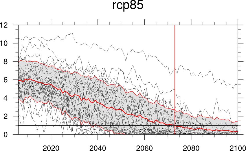
4208 A. Lauer et al.: Earth System Model Evaluation Tool (ESMValTool) v2.0
Table 1. Continued.
Recipe name Section Description Variables Diagnostic scripts Observational datasets
recipe_deangelis15nat.yml 3.3.5 constraint on hydro- hfss, lvp, prw, deangelis15nat/deangelis1b.py ERA-Interim (prw),
logic cycle intensifica- rlnst, rlnstcs, deangelis15nat/deangelis2.py RSS (prw), CERES-
tion (DeAngelis et al., rsnst, rsnstcs, deangelis15nat/deangelis3.py EBAF (rlnstcs, rsnst,
2015) rsnstcsnorm, rsnstcs, rsnstcsnorm)
tas
recipe_li2017natcc.yml 3.3.5 emergent constraint on pr, ts, ua, va emergent_constraints/lif1.py GPCP (pr)
the future Indian sum-
mer monsoon precipi-
tation following Li et
al. (2017)
Section 3.4: climate model projections
recipe_wenzel16jclim.yml 3.4.1 constraint on austral jet asr, ps, ta, uajet austral_jet/asr.ncl ERA-Interim (ps, ta,
position in future pro- (ua), va austral_jet/main.ncl ua, va), CERES-EBAF
jections mder/absolute_correlation.ncl (asr)
mder/regression_stepwise.ncl
mder/select_for_mder.ncl
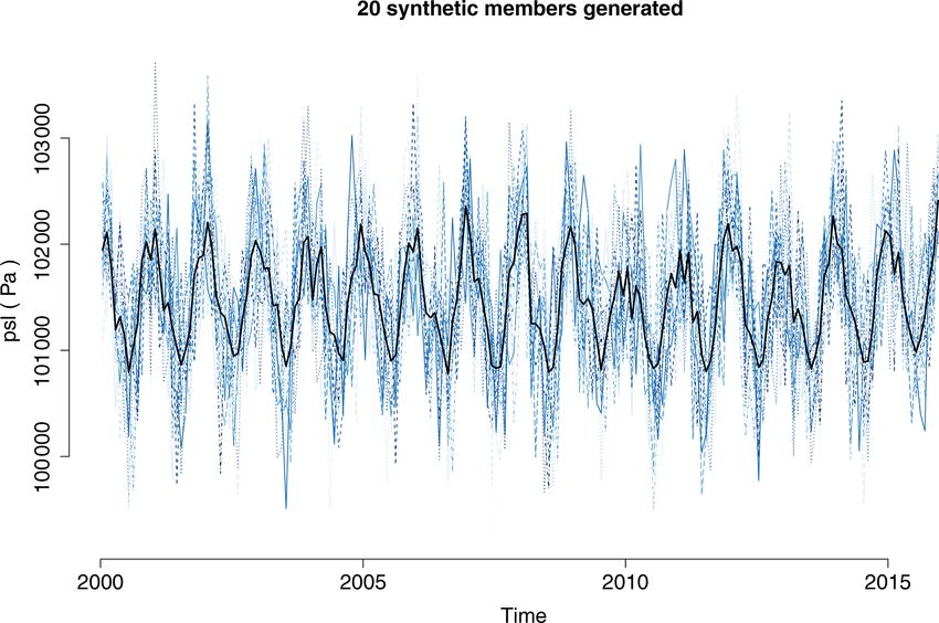
recipe_toymodel.yml 3.4.2 recipe for generating psl (example) magic_bsc/toymodel.R ERA-Interim (psl)
synthetic observations
based on the model
presented in Weigel et
al. (2008)
recipe_collins13ipcc.yml 3.4.3 selected figures from areacello, clt, ipcc_ar5/ch12_calc_IAV_for_ HadISST (sic)
IPCC AR5, chap. 12 evspsbl, hurs, stippandhatch.ncl
(Collins et al., 2013): mrro, mrsos, ipcc_ar5/ch12_calc_map_diff_mmm_
mainly difference maps pr, psl, rlut, stippandhatch.ncl
between future and rsut, rtmt, sic, ipcc_ar5/ch12_calc_zonal_cont_
present snw, sos, ta, tas, diff_mmm_stippandhatch.ncl
thetao, ua ipcc_ar5/ch12_map_diff_each_model_
fig12-9.ncl
ipcc_ar5/ch12_plot_map_diff_
mmm_stipp.ncl
ipcc_ar5/ch12_plot_ts_line_mean_
spread.ncl
ipcc_ar5/ch12_plot_zonal_diff_
mmm_stipp.ncl
ipcc_ar5/ch12_snw_area_change_fig12-
32.ncl
ipcc_ar5/ch12_ts_line_mean_spread.ncl
seaice/seaice_ecs.ncl
seaice/seaice_yod.ncl
recipe_seaice.yml 3.4.4 time series of sea ice areacello, sic seaice/seaice_aux.ncl HadISST (sic)
area and extent, sea seaice/seaice_ecs.ncl
ice extent trend distri- seaice/seaice_trends.ncl
butions, year of near seaice/seaice_tsline.ncl
disappearance of Arctic seaice/seaice_yod.ncl
sea ice, emergent con-
straint on YOD (Mas-
sonnet et al., 2012)
volves saving only one variable per file and adding metadata user guide available at https://docs.esmvaltool.org/en/latest/
such as coordinates (e.g., longitude, latitude, pressure level, input.html#observations (last access: 18 June 2020).
time) and attributes (e.g., variable standard and long names,
units, dimensions) according to the CMOR standard to the
dataset(s). The second way is to implement specific “fixes” 3 Overview of recipes included in ESMValTool v2.0 for
for this dataset in which case the CMORizing is performed emergent constraints and future projections
“on the fly” during the execution of an ESMValTool recipe.
For details on both methods, we refer to the ESMValTool In this section, all diagnostics and metrics newly added to
ESMValTool v2.0 for analysis of future projections from
ESMs as well as the emergent constraints implemented are
Geosci. Model Dev., 13, 4205–4228, 2020 https://doi.org/10.5194/gmd-13-4205-2020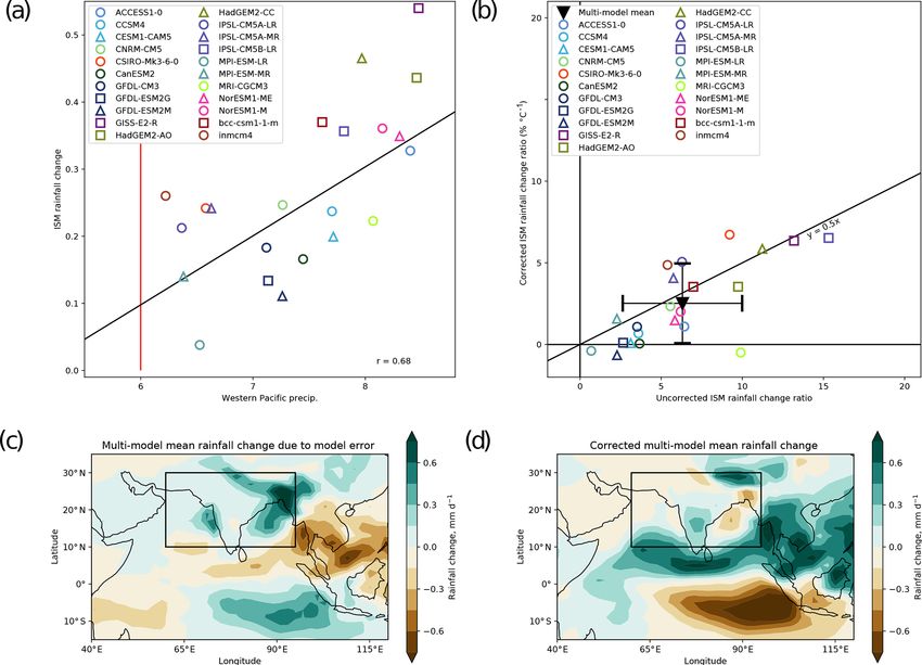
A. Lauer et al.: Earth System Model Evaluation Tool (ESMValTool) v2.0                                                             4209

Table 2. Emergent constraints implemented in ESMValTool v2.0 and observational datasets used.

      Reference                      Constrained parameter     Description/observed quantity       Observational datasets
      Brient and Schneider (2016)    ECS                       covariance of shortwave cloud       HadISST (ts), ERA-Interim
                                                               reflection                          (hur), CERES-EBAF (rsut,
                                                                                                   rsutcs, rsdt)
      Cox et al. (2018)              ECS                       global temperature variability      HadCRUT4 (tasa)
      DeAngelis et al. (2015)        hydrologic cycle inten-   radiative fluxes and precipitable   CERES-EBAF (rsdscs, rsdt,
                                     sification                water                               rsuscs, rsutcs), RSS (prw),
                                                                                                   ERA-Interim (prw)
      Hall and Qu (2006)             snow-albedo effect        springtime snow-albedo feed-        ISCCP-FH (alb, rsdt), ERA-
                                                               back values in climate change       Interim (tas)
                                                               vs. springtime values in the sea-
                                                               sonal cycle in transient climate
                                                               change
      Massonnet et al. (2012)        YOD                       year of disappearance (YOD)         HadISST (sic)
                                                               of September Arctic sea ice vs.
                                                               mean sea ice extent or trend in
                                                               sea ice extent
      Li et al. (2017)               future Indian summer      present-day precipitation over      GPCP (pr)
                                     monsoon precipitation     the tropical western Pacific
      Lipat et al. (2017)            ECS                       climatological Hadley cell ex-      ERA-Interim (va)
                                                               tent
      Sherwood et al. (2014)         ECS                       lower tropospheric mixing in-       ERA-Interim (hur, ta, wap)
                                                               dex (LTMI)
      Tian (2015)                    ECS                       southern ITCZ index, tropi-         TRMM (pr), AIRS (hus)
                                                               cal mid-tropospheric humidity
                                                               asymmetry index
      Volodin (2008)                 ECS                       difference between tropical and     ISCCP-D2 (clt)
                                                               midlatitude cloud fraction
      Wenzel et al. (2014)           climate–carbon    cycle   long-term sensitivity of tropical   NCEP (tas), GCP (nbp, fgco2)
                                     feedback (γLT )           land carbon storage to climate
                                                               warming
      Wenzel et al. (2016a)          land photosynthesis (β)   carbon cycle – CO2 concentra-       NOAA station measurements
                                                               tion feedback                       Alaska and Hawaii (co2)

described and illustrated with examples using results from           tails on the technical infrastructure of the tool including ac-
the CMIP5 model ensemble (Taylor et al., 2012). The ESM-             cepted data formats, data reference syntax (DRS) used for
ValTool workflow is controlled by configuration files called         directory and file name conventions, available preprocessor
“recipes”, which define all input datasets, preprocessing            functions, etc., we refer again to Righi et al. (2020). Fur-
steps and diagnostics to run (for details we refer to Righi          ther information can be found in the ESMValTool user guide,
et al., 2020). An overview of all recipes described in this pa-      which documents all technical aspects of the tool as well
per including a short description, the variables processed, the      as all available diagnostics; see https://docs.esmvaltool.org/
names of the diagnostic scripts and observations is given in         (last access: 1 September 2020).
Table 1.
   All diagnostics output one or more NetCDF file(s) con-
taining the results of the analysis that are then visualized in      3.1    Calculations of multi-model products
the figure(s) created. The file format of the figures can be
defined in the user configuration file and includes common           Multi-model means are commonly used to project climate
formats such as *.png, *.pdf, *.ps and *.eps. For more de-           change (IPCC, 2013, 2007) and are thus a useful quantity to

https://doi.org/10.5194/gmd-13-4205-2020                                                  Geosci. Model Dev., 13, 4205–4228, 2020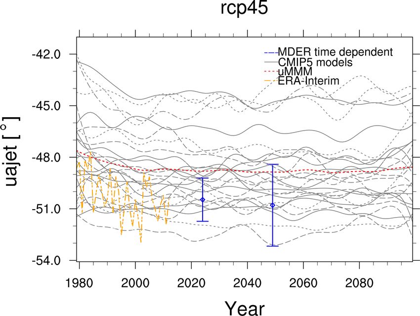
4210 A. Lauer et al.: Earth System Model Evaluation Tool (ESMValTool) v2.0
calculate in support of diagnostics included in the ESMVal- new equilibrium (Gregory et al., 2004). Climate models of
Tool. the CMIP5 model ensemble simulated an ECS ranging be-
The recipe recipe_multimodel_products.yml computes the tween 2.1 and 4.7 K (Flato et al., 2013). Using all avail-
multi-model ensemble mean for a set of models selected by able evidence of that time, IPCC AR5 assessed a “likely”
the user for individual variables and different temporal reso- range of ECS between 1.5 and 4.5 K in 2013 (IPCC, 2013).
lutions (annual, seasonal, monthly). For this, all data are re- recipe_ecs.yml uses a regression method proposed by Gre-
gridded to the same horizontal grid. In the example shown in gory et al. (2004) to calculate ECS. Using the total radiative
Fig. 1, all models are regridded to the grid of BCC-CSM1- forcing F caused by the doubling of atmospheric CO2 con-
1 using a linear interpolation scheme. This task is done by centration and the climate feedback parameter λ, ECS is de-
the ESMValTool’s preprocessor and defined in the recipe de- fined as ECS = F /λ. Both of these variables can be assessed
pending on the application and user requirements. The user- by linear regression of the equation for radiative balance
definable configuration options include definition of the tar- N = F −λ1T , where N is the net radiation flux at the top of
get grid (e.g., 2.5◦ × 2.5◦ ) and regridding scheme (e.g., lin- the atmosphere (TOA) and 1T the global mean near-surface
ear, nearest, area weighted). Regridding/interpolation of the air temperature change. N and 1T are both given as global
input data in time is currently not supported. For further de- and annual mean differences between the abrupt quadrupled
tails, we refer to the ESMValTool user guide (https://docs. CO2 simulation and the linear regression of the pre-industrial
esmvaltool.org/, last access: 1 September 2020). After select- control run. Figure 3 illustrates this regression for the CMIP5
ing the region (rectangular region defined by the lowermost multi-model mean. Moreover, it shows that the assumption
and uppermost longitudes and latitudes), the mean for the se- of a linear climate feedback parameter is only an approx-
lected reference period is subtracted from the time series in imation. Using only the first 20 years (last 130 years) in-
order to obtain the anomalies for the desired period. In addi- stead of all 150 years of the abrupt quadrupled CO2 simu-
tion, the recipe computes the percentage of models agreeing lations results in a stronger (weaker) feedback, which again
on the sign of this anomaly, thus providing some information leads to a lower (higher) ECS. This demonstrates the differ-
on the robustness of the climate change signal. ent response of the climate system at different timescales,
The output of the recipe consists of a contour map show- i.e., non-linear feedback processes. This diagnostic requires
ing the time average of the multi-model mean anomalies and the input variables near-surface air temperature (tas), TOA
stippling to indicate locations where the percentage of mod- incoming shortwave radiation (rsdt), TOA outgoing short-
els agreeing on the sign of the multi-model mean anomaly wave radiation (rsut) and TOA outgoing longwave radiation
exceeds a threshold selected by the user (Fig. 1). The exam- (rlut) from abrupt4xCO2 (quadrupling of CO2 compared to
ple in Fig. 1 shows a warming over the continents in the range pre-industrial conditions) and piControl (pre-industrial con-
of 1–2 K which is more pronounced than the warming over trol) simulations.
the ocean which is mostly in the range of 0.5–1.5 K in this Figure 9.42a of Flato et al. (2013) shows the globally av-
scenario. The example also shows that the models largely eraged mean near-surface air temperature (GMSAT) for the
agree on the sign of the temperature change with the most historical period of 1961–1990 plotted vs. ECS of several
prominent exceptions found in parts of the Southern Ocean, CMIP5 models. The latter quantity can be calculated by a re-
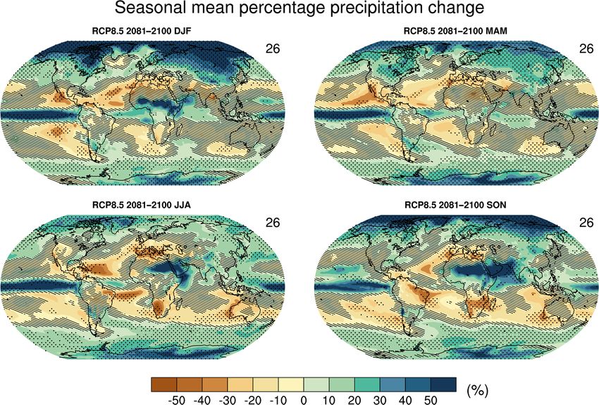
Greenland and the North Atlantic. Furthermore, a time se- gression method based on Gregory et al. (2004) as outlined
ries of the area-weighted mean anomalies is plotted. For the above. A similar figure produced with recipe_flato13ipcc.yml
plots, the user can select the length of the running window implemented in ESMValTool v2.0 shows that there are no
for temporal smoothing and choose to display either the en- distinctive correlations between the historical surface tem-
semble mean with a light shading to represent the spread of peratures and the ECS, which suggests that the ECS is not
the ensemble or each individual model separately (Fig. 2). very sensitive to errors in the current climate in contrast to
The example in Fig. 2 shows an increase in global average other sources of uncertainty (Fig. 4).
June temperatures up to about 2060 when temperatures start The TCR is defined as the global and annual mean near-
to level off. By 2100, the four CMIP5 example models (MPI- surface air temperature anomaly in the 1pctCO2 simulation
ESM-MR, CNRM-CM5, BCC-CSM1-1 and IPSL-CM5A- (1 % increase in CO2 per year) for a 20-year period cen-
LR) show a spread in temperature increase for the RCP2.6 tered at the time of CO2 doubling, i.e., using the years 61 to
scenario ranging from 0.7 to about 1.8 K. 80 after the start of the simulation. The temperature anoma-
lies are calculated by subtracting a linear fit to the piControl
3.2 ECS and TCR run for all 140 years from the 1pctCO2 experiment prior to
the TCR calculation (Gregory and Forster, 2008). Figure 5
The ECS is an important metric to assess the future warm- shows (a) a time series of the 1pctCO2 near-surface temper-
ing of the climate system. It is defined as the change in ature anomalies from MIROC-ESM used to obtain TCR and
global mean near-surface air temperature as a result of a dou- (b) TCR values for different CMIP5 models calculated with
bling of the atmospheric CO2 concentration compared to pre- recipe_tcr.yml.
industrial conditions after the climate system has reached a
Geosci. Model Dev., 13, 4205–4228, 2020 https://doi.org/10.5194/gmd-13-4205-2020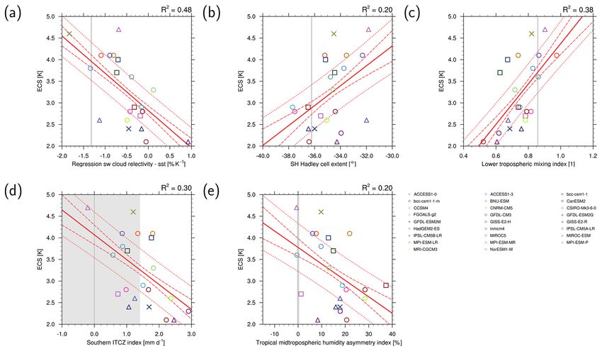
A. Lauer et al.: Earth System Model Evaluation Tool (ESMValTool) v2.0                                                                 4211

Figure 1. Multi-model mean of projected future June near-surface air temperature anomalies (2006–2099) compared with the period of
1961–1990 (colors). Crosses indicate that the 80 % of models agree with the sign of the multi-model mean anomaly. The models used in this
example are BCC-CSM1-1, MPI-ESM-MR and MIROC5 (r1i1p1 ensembles) for the RCP2.6 scenario. All models have been regridded to
the BCC-CSM1-1 grid using a linear interpolation scheme. See Sect. 3.1 for details on recipe_multimodel_products.yml.

                                                                       Figure 3. Gregory plot to approximate the ECS (Gregory et al.,
                                                                       2004). Shown is the relationship between the differences in global
                                                                       and annual mean top-of-the-atmosphere net downward radiative
                                                                       flux N (W m−2 ) and global and annual mean near-surface air tem-
                                                                       perature anomalies 1T (K) for the CMIP5 multi-model mean.
                                                                       Anomalies are calculated as difference between the abrupt4xCO2
                                                                       experiment (quadrupling of CO2 ) and the pre-industrial control run
                                                                       (piControl). The blue dots show the first 20 years of the simulation;
Figure 2. Time series of global average near-surface air temper-
                                                                       the orange dots show the last 130 years. A linear regression using
ature anomalies in June for the period of 2006–2099 (RCP2.6
                                                                       only the first 20 years (blue line) instead of all 150 years (black
scenario) compared to the reference period of 1961–1990.
                                                                       line) results in a stronger feedback (and thus lower ECS). Using the
The individual models are shown as colored lines; the multi-
                                                                       last 130 years only (orange line) results in a weaker feedback (i.e.,
model mean is shown in black. See Sect. 3.1 for details on
                                                                       higher ECS). See Sect. 3.2 for details on recipe_ecs.yml.
recipe_multimodel_products.yml.

https://doi.org/10.5194/gmd-13-4205-2020                                                   Geosci. Model Dev., 13, 4205–4228, 2020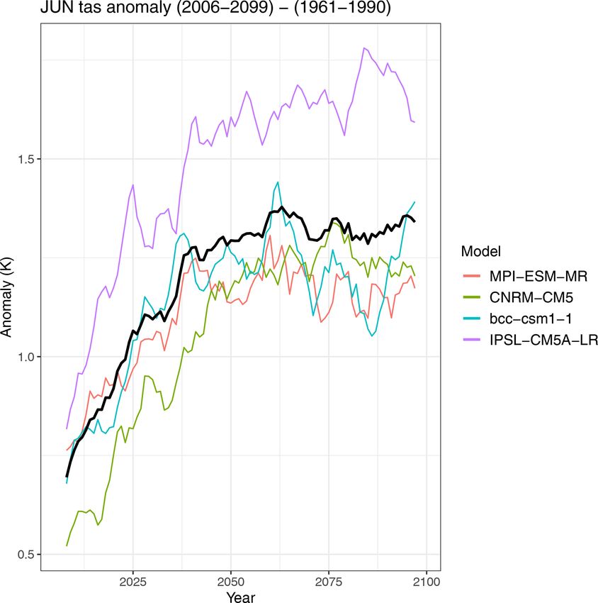
4212                                               A. Lauer et al.: Earth System Model Evaluation Tool (ESMValTool) v2.0

Figure 4. Globally averaged near-surface air temperature (GMSAT) of the historical period of 1961–1990 vs. the ECS for several CMIP5
models. Similar to Fig. 9.42a of Flato et al. (2013) and produced with recipe_flato13ipcc.yml; see details in Sect. 3.2.

Figure 5. (a) Time series of temperature anomalies from MIROC-ESM experiment 1pctCO2 (1 % increase in CO2 per year) compared to the
piControl simulation. (b) Transient climate response (in K) for CMIP5 models calculated with the method by Gregory and Forster (2008).
For details on recipe_tcr.yml, see Sect. 3.2.

3.3    Emergent constraints                                          certainties in climate projections and can help guide model
                                                                     development by highlighting processes that are crucial to ex-
An emergent constraint utilizes an ensemble of ESMs to-              plaining the magnitude and spread of the modeled future cli-
gether with observational data to constrain a simulated future       mate change. Emergent constraints can also help point out
Earth system feedback. A prerequisite for an emergent con-           the need for more and/or more reliable observations.
straint is a robust relationship between, for example, changes          We would like to note that a limitation of the emergent
occurring on seasonal or interannual timescales and changes          constraints as currently implemented into the ESMValTool
found in ESM simulations of anthropogenically forced cli-            is that model interdependency, as in the original studies, is
mate change (Eyring et al., 2019). If such a relationship can        not explicitly taken into account. As some modeling groups
be explained by a plausible physical mechanism, an obser-            share model components or code, the models are not all in-
vational constraint of multi-model projections of quantities         dependent. Duplicated code, as well as identical forcing and
that cannot be observed directly might be possible. Such a           validation data in multiple models, is expected to lead to
non-observable quantity is, for instance, ECS. The technique         an overestimation of the sample size of a model ensemble
of emergent constraints offers the possibility to reduce un-

Geosci. Model Dev., 13, 4205–4228, 2020                                               https://doi.org/10.5194/gmd-13-4205-2020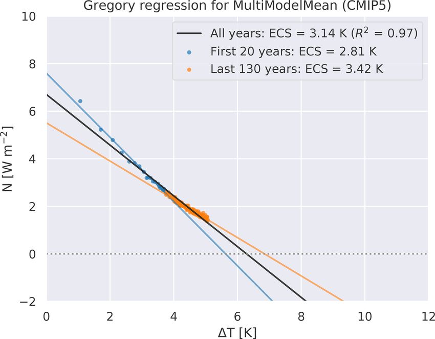
A. Lauer et al.: Earth System Model Evaluation Tool (ESMValTool) v2.0                                                          4213

and may result in spurious correlations (Sanderson et al.,           Covariance of shortwave cloud reflection
2015). As a possible approach, future implementations of
these emergent constraints could, for example, apply a model         This emergent constraint uses the models’ correlation of
weighting based on a model’s interdependence (e.g., Knutti           tropical low-level cloud (TLC) reflection with the underlying
et al., 2017) or simply reduce the ensemble size by taking           SST to constrain ECS (Brient and Schneider, 2016). The def-
into account only models that are above a given yet-to-be-           inition and calculation of the individual terms follows Brient
defined interdependence score.                                       and Schneider (2016): TLC regions are defined as the 25 %
   Table 2 summarizes the emergent constraints that have             ocean areas between 30◦ S and 30◦ N with the lowest 500 hPa
been implemented in ESMValTool (v2.0) including the ob-              relative humidity. TLC reflection is calculated as the ratio of
servational datasets used and are described in the following.        top-of-the-atmosphere shortwave cloud radiative forcing and
                                                                     insolation, both averaged over the TLC region. This is then
3.3.1   Emergent constraints on effective climate                    used to calculate the regression coefficients of deseasonal-
        sensitivity                                                  ized variations of TLC shortwave reflection and sea surface
                                                                     temperature in % per K used as an emergent constraint. In the
recipe_ecs_scatter.yml calculates five emergent constraints          example shown in Fig. 6a, data from the CMIP5 historical
for ECS (see Table 2). These are briefly described in                simulations between 1980 and 2005 are used for the models,
Sect. 3.3.1 (“Covariance of shortwave cloud reflection” to           observational/reanalysis data used in Fig. 6 are ERA-Interim
“Tropical mid-tropospheric humidity asymmetry index”).               (Dee et al., 2011) for relative humidity, HadISST (Rayner
The ECS values from the models are pre-calculated with               et al., 2003) for sea surface temperatures and CERES-EBAF
recipe_ecs.yml (see Sect. 3.2) or can be taken from literature.      (Ed2.7) (Loeb et al., 2012) for top-of-the-atmosphere radia-
The diagnostic calculates ECS vs. selected constraining pa-          tive fluxes.
rameters, such as the climatological Hadley cell extent from
models, and fits a linear regression line to the data. If avail-     Climatological Hadley cell extent
able, the observational uncertainty of a given observational
dataset can be estimated. For this, the standard error of the        Lipat et al. (2017) found that the climatological mean
observations is subtracted or added from or to the means be-         Hadley cell (HC) edge latitude from CMIP5 models corre-
fore calculating the observational value (estimated minimum          lates with ECS. The HC edge latitude is calculated from
or maximum, respectively). In addition to the scatter plots          first two grid cells from the Equator going south where the
of ECS vs. constraining parameter calculated by the diag-            zonal average 500 hPa mass stream function changes sign
nostic, the diagnostic also outputs the 25 %/75 % confidence         from negative to positive (downward branch of the HC).
intervals of the regression (i.e., uncertainty of the fit) and the   The mass stream function is calculated from climatological
25 %/75 % prediction intervals of the regression (i.e., mea-         December–January–February (DJF) means of the meridional
sure for the quality of the linear fit). By definition, 50 % of      wind fields. The correlation of the climatological HC extent
all model data points are within the 25 %/75 % prediction in-        with ECS found in CMIP5 models is explained by obser-
terval of the regression line. Examples of the different scat-       vations that show a correlation of variability in midlatitude
ter plots that can be created by recipe_ecs_scatter.yml are          clouds and cloud radiative effects with poleward HC expan-
shown in Fig. 6. It should be noted that because a different         sion (Lipat et al., 2017). For the example shown in Fig. 6b,
set of CMIP5 models might be used in the figures compared            CMIP5 data from historical simulations and ERA-Interim
to the originally published emergent constraints, the figures        (Dee et al., 2011) are used as a reference dataset for the years
could show some deviations to the ones published in litera-          1980–2005.
ture. While the emergent constraints shown in Fig. 6a, c, d,
e suggest ECS values in the upper range of the values given          Lower tropospheric mixing index
in IPCC AR5 (IPCC, 2007, 1.5 to 4.5 K), the emergent con-
straint shown in Fig. 6b suggests an ECS value in the lower          Following Sherwood et al. (2014), the lower tropospheric
range of the IPCC AR5 values.                                        mixing index (LTMI) can be used to constrain ECS and is
   In addition to these five emergent constraints,                   calculated as the sum of small-scale mixing S and the large-
recipe_cox18nature.yml implements an emergent con-                   scale component of mixing D. S is calculated from relative
straint for ECS based on global temperature vari-                    humidity (RH) and temperature (T ) differences between 700
ability (Sect. 3.3.1, “Global temperature variability”),             and 850 hPa and averaged over a tropical region between
recipe_ecs_constraints.yml an emergent constraint based              30◦ S and 30◦ N defined by the upper quartile of the an-
on the difference between tropical and midlatitude cloud             nual mean 500 hPa ascent rate within ascending regions: S =
fraction (Sect. 3.3.1, “Difference between tropical and              (1RH700−850 /100 % − 1T700−850 /9 K)/2. The large-scale
midlatitude cloud fraction”).                                        component of mixing is the ratio of shallow to deep over-
                                                                     turning: D = h1H (1)H (−ω1 )i/h−ω2 H (−ω2 )i with ω1 the
                                                                     average of the vertical velocity at 850 and 700 hPa, ω2 the av-

https://doi.org/10.5194/gmd-13-4205-2020                                               Geosci. Model Dev., 13, 4205–4228, 2020
4214                                                    A. Lauer et al.: Earth System Model Evaluation Tool (ESMValTool) v2.0

Figure 6. Scatter plots of ECS vs. (a) covariance of shortwave cloud reflection (Brient and Schneider, 2016), (b) Southern Hemisphere
(SH) climatological Hadley cell extent (Lipat et al., 2017), (c) lower tropospheric mixing index (LTMI) (Sherwood et al., 2014), (d) south-
ern Intertropical Convergence Zone (ITCZ) index (Tian, 2015) and (e) tropical mid-tropospheric humidity asymmetry index (Tian, 2015)
for CMIP5 models (symbols). The vertical gray lines represent the observations; the shaded areas in light gray represent observational un-
certainties (if available). The solid red lines represent the regression lines, the dashed red lines the 25 %/75 % confidence intervals of the
regression and the dotted red lines the 25 %/75 % prediction intervals of the regression. Similar to (a) Fig. 6 of Brient and Schneider (2016),
(b) Fig. 4 of Lipat et al. (2017), (c) Fig. 5c of Sherwood et al. (2014), (d) Fig. 2 of Tian (2015) and (e) Fig. 4c of Tian (2015). For details on
recipe_ecs_scatter.yml, see Sect. 3.3.1.

erage of the vertical velocity at 600, 500 and 400 hPa, H the              mm d−1 . The southern ITCZ index is used to quantify the
step function and h. . .i the average over the tropical ocean              double-ITCZ bias in CMIP3 and CMIP5 models and has
region 30◦ S–30◦ N, 160◦ W–30◦ E. The lower tropospheric                   been found to correlate with ECS (Tian, 2015). In the ex-
mixing index is calculated as LTMI = S + D. Sherwood et                    ample shown in Fig. 6d, the ITCZ index has been calcu-
al. (2014) explain the correlation between LTMI and ECS in                 lated from CMIP5 historical model simulations averaged
CMIP3 and CMIP5 models by convective mixing between                        over the years 1980–2005. Tropical Rainfall Measuring Mis-
the lower and middle tropical troposphere dehydrating low-                 sion (TRMM) (Huffman et al., 2007) satellite data (v7) aver-
level cloud layers at an increasing rate as climate warms.                 aged over the years 1998–2013 have been used as observa-
They argue that this rate of increase depends on initial mixing            tional reference.
strength, which links the mixing to clouds feedbacks and thus
ECS. Figure 6c shows an example of this emergent constraint                Tropical mid-tropospheric humidity asymmetry index
applied to CMIP5 historical simulations using ERA-Interim
data (Dee et al., 2011) as reference data. All datasets in this            The strong link found in CMIP3 and CMIP5 models between
example cover the time period of 1980–2005.                                the double-ITCZ bias and simulated moisture, precipitation,
                                                                           clouds and large-scale circulation allows the double-ITCZ
Southern ITCZ index                                                        bias and thus ECS to also be related to mid-tropospheric
                                                                           humidity over the tropical Pacific (Tian, 2015). As shown
The southern Intertropical Convergence Zone (ITCZ) index                   by Tian (2015), spatial patterns of mid-tropospheric humid-
(Bellucci et al., 2010; Hirota et al., 2011) is defined as the             ity and precipitation are similar as both are related to the
climatological annual mean precipitation bias averaged over                ITCZ. This allows defining a tropical mid-tropospheric hu-
the south-eastern Pacific (30◦ S–0◦ , 150–100◦ W) given in                 midity asymmetry index to quantify the double-ITCZ bias

Geosci. Model Dev., 13, 4205–4228, 2020                                                       https://doi.org/10.5194/gmd-13-4205-2020
A. Lauer et al.: Earth System Model Evaluation Tool (ESMValTool) v2.0 4215
in models and consequently constrain ECS. This index is
defined as relative bias in simulated annual mean 500 hPa
specific humidity compared with observations ((model −
observation)/observation·100 %) averaged over the Southern
Hemisphere (SH) tropical Pacific (30◦ S–0◦ , 120◦ E–80◦ W)
minus the bias averaged over the Northern Hemisphere (NH)
tropical Pacific (20◦ N–0◦ , 120◦ E–80◦ W) (Tian, 2015). The
example for the tropical mid-tropospheric humidity asymme-
try index shown in Fig. 6e is calculated from CMIP5 his-
torical runs averaged over the years 1980–2005 and AIRS
(v5) satellite data (Susskind et al., 2006) averaged over the
years 2003–2010 as observational reference data.
Global temperature variability
Cox et al. (2018) propose an emergent constraint for the ECS
using global temperature variability. The latter is defined by
a metric ψ which can be calculated from the global tempera- Figure 7. Emergent constraint for ECS. Shown is the relation-
ture variance (in time) σT and the 1-year-lag autocorrelation ship between ECS and the temperature variability metric ψ pro-
of the global temperature α1T by posed by Cox et al. (2018). Letters show individual CMIP5 mod-
els (for nomenclature details, see original publication) with lower-
σT sensitivity models in green and higher-sensitivity models in purple.
ψ=√ . (1) The black lines show the linear fit including the prediction error and
− ln(α1T )
the vertical blue lines indicate the observational mean and standard
Using the simple “Hasselmann model” (Hasselmann, 1976), deviation given by the HadCRUT4 dataset. Similar to Fig. 2 of Cox
Cox et al. (2018) showed that ψ is linearly correlated with et al. (2018) and produced with recipe_cox18nature.yml (see details
in Sect. 3.3.1, “Global temperature variability”).
ECS in CMIP5 data. Since calculation of ψ only depends
on the temporal evolution of the global surface tempera-
ture, there are many observational datasets available. In the
original publication, data from HadCRUT4 (Morice et al., with recipe_ecs_constraints.yml, which uses CMIP5 histori-
2012) are used to construct the emergent relationship. In the cal runs averaged between 1980 and 2000 (Fig. 8). The ob-
ESMValTool, this is reproduced by recipe_cox18nature.yml, served values are based on ISCCP-D2 data and are taken
which only needs two variables: historical near-surface air from Volodin (2008).
temperature (tas) and ECS (see Sect. 3.2). The emergent re-
lationship between ECS and ψ is shown in Fig. 7 includ- 3.3.2 Emergent constraints on the carbon cycle
ing means and confidence intervals. The constrained range
of ECS based on this plot is 2.2 to 3.4 K with a 66 % confi- Uncertainties in projections of future temperature using
dence interval, similar to Cox et al. (2018). ESMs are high, in a large part due to uncertainties of emis-
sions and feedbacks. Within the carbon cycle, feedbacks are
Difference between tropical and midlatitude cloud usually split into the carbon cycle – climate feedback γ ,
fraction which quantifies carbon to climate change, and the carbon
cycle – CO2 concentration feedback β, which is the carbon
Volodin (2008) proposes an emergent constraint for ECS sensitivity to atmospheric CO2 (Friedlingstein et al., 2006).
based on the distribution of clouds in global climate mod- γ is a positive feedback as climate warming reduces the ef-
els. The study finds that models with high climate sensi- ficiency of CO2 absorption by the land and ocean, leading to
tivity show a higher total cloud cover over the southern more of the emitted carbon staying in the atmosphere, which
midlatitudes and a lower total cloud cover over the tropics in turn leads to additional warming. In contrast, β is a neg-
than the multi-model average. Thus, the difference in trop- ative feedback because of the so-called CO2 fertilization ef-
ical total cloud cover (between 28◦ S and 28◦ N) and the fect, where plants take up a higher amount of CO2 for pho-
SH midlatitude total cloud cover (between 56 and 36◦ S) tosynthesis with increasing atmospheric CO2 concentrations.
is negatively correlated with ECS. The original publication Efforts have been made to reduce the uncertainties of these
uses the CMIP3 ensemble and the International Satellite two carbon cycle feedback parameters.
Cloud Climatology Project (ISCCP)-D2 dataset (Rossow and Wenzel et al. (2014) employed the emergent constraint
Schiffer, 1991) as observational reference, but the relation- described by Cox et al. (2013) for the long-term sensitiv-
ship also holds when using CMIP5 models. In the ESM- ity of tropical land carbon storage to climate warming (γLT )
ValTool, this emergent constraint for ECS can be produced to the interannual sensitivity of atmospheric CO2 to interan-
https://doi.org/10.5194/gmd-13-4205-2020 Geosci. Model Dev., 13, 4205–4228, 20204216 A. Lauer et al.: Earth System Model Evaluation Tool (ESMValTool) v2.0
Figure 8. ECS vs. difference in total cloud cover between the trop-
ics (28◦ S–28◦ N) and southern midlatitudes (56–36◦ S) for CMIP5
models (orange dots). The orange line and shaded area show the
Figure 9. Relationship between long-term sensitivity of tropi-
linear regression line and its 95 % uncertainty range (estimated via
cal land carbon storage to climate warming (γLT ) and short-term
bootstrapping). Together with the observational estimate (vertical
sensitivity of atmospheric CO2 to interannual temperature vari-
blue line and shaded area), this can be used as an emergent con-
ability (γIAV ) for CMIP5 models (markers with horizontal and
straint for ECS (Volodin, 2008). The observational range is based
vertical error bars) using the historical simulation. The red line
on ISCCP-D2 data (Rossow and Schiffer, 1991) and taken from
shows the linear regression through the CMIP5 models; the ver-
Volodin (2008). Similar to Fig. 3a of Volodin (2008) and produced
tical gray area shows the range of observed γIAV . Produced with
with recipe_ecs_constraints.yml (see details in Sect. 3.3.1, “Differ-
recipe_wenzel14jgr.yml, similar to Fig. 5a of Wenzel et al. (2014)
ence between tropical and midlatitude cloud fraction”).
(for details, see Sect. 3.3.2).
nual tropical temperature variability (γIAV ) in CMIP5 mod- run this recipe is gross primary productivity (GPP) in the
els. The analysis from this paper can be reproduced using esmFixClim1 simulations, as well as the atmospheric CO2
recipe_wenzel14jgr.yml with the emergent relationship be- concentration (co2) from emission-driven historical simula-
ing able to reduce the range of projected γLT (Fig. 9). In- tions. Observations used are the atmospheric CO2 concen-
put variables include net primary productivity (nbp), surface trations at Point Barrow (BRW; 71.3◦ N, 156.6◦ W), Alaska,
temperature (tas), gas exchange flux of CO2 into the ocean and Cape Kumukahi, Hawaii (KMK; 19.5◦ N, 155.6◦ W)
(fgco2) from the experiment 1pctCO2, nbp, fgco2, tas from (NOAA, 2018).
the emission-driven historical simulations (esmHistorical),
as well as nbp from the esmFixClim1 (carbon cycle sees CO2 3.3.3 Emergent constraints on the year of
concentration increase but radiation does not) simulations. disappearance of September Arctic sea ice
The different simulations are included in γIAV , which is es-
timated from both the 1pctCO2 experiment and the esmHis- This sea ice diagnostic produces scatter plots of (a) mean
torical simulation, and then compared in the paper. The de- of and (b) trend in historical September Arctic sea ice ex-
fault observational datasets are NCEP reanalysis (Kalnay et tent (SSIE) vs. the first year of disappearance (YOD). Here,
al., 1996) for the surface temperature and the Global Carbon YOD is defined as the first of five consecutive years in which
Project (GCP; Le Quere et al., 2015) for the carbon fluxes. the Arctic SSIE drops below 1 million km2 (Wang and Over-
Wenzel et al. (2016a) developed an emergent constraint for land, 2009). Sea ice extent is defined in the diagnostic as the
β on land in the extratropics and northern midlatitudes con- total area of all grid cells in which the sea ice concentra-
straining the projected land photosynthesis with changes in tion is 15 % or larger, Arctic is defined as the region north of
the seasonal cycle of atmospheric CO2 . The figures from this 60◦ N. The annual minimum Arctic sea ice extent typically
paper can be reproduced with recipe_wenzel16nat.yml, with occurs in September. For this reason, September mean sea ice
Fig. 10 showing the emergent constraint reproduced with the quantities are commonly used in literature for analyses of the
ESMValTool. The unconstrained CO2 fertilization effect lies timing of an ice-free Arctic (e.g., Massonnet et al., 2012; Sig-
at 40 ± 20 %, which can be narrowed down to 37 ± 9 % in mond et al., 2018). The two scatter plots in Fig. 11a and b are
high latitudes and 32±9 % in the extratropics with this emer- similar to those in Fig. 12.31a/c of Collins et al. (2013), re-
gent constraint. Input variables from the models needed to spectively. In addition, the diagnostic produces a scatter plot
Geosci. Model Dev., 13, 4205–4228, 2020 https://doi.org/10.5194/gmd-13-4205-2020A. Lauer et al.: Earth System Model Evaluation Tool (ESMValTool) v2.0 4217
Figure 10. (a) Correlations between the sensitivity of the CO2 amplitude to annual mean CO2 increases at Point Barrow, Alaska (abscissa),
and the high-latitude (60–90◦ N) CO2 fertilization of GPP at twice the CO2 . The gray shading shows the range of the observed sensitivity.
The red line shows the linear best fit across the CMIP5 ensemble together with the prediction error (orange) and error bars show the standard
deviation for each data point. (b) The probability density function for the unconstrained CO2 fertilization of GPP (black, dotted) and the
conditional probability density function arising from the emergent constraint (red). Produced with recipe_wenzel16nat.yml, similar to Fig. 3
of Wenzel et al. (2016a) (for details, see Sect. 3.3.2).
of mean SSIE vs. trend in historical SSIE, similar to Fig. 2 – (ordinate values) the change in April αs (future projec-
of Massonnet et al. (2012). In the example shown in Fig. 11, tion – historical) averaged over NH land masses pole-
HadISST data (Rayner et al., 2003) over the time period of ward of 30◦ N is divided by the change in April Ts (fu-
1960–2005 have been used as a reference dataset for com- ture projection – historical) averaged over the same re-
parison with CMIP5 results. The figure shows that while the gion. The change in αs (or Ts ) is defined as the dif-
individual models spread widely around the observed mean ference between 22nd century mean αs (Ts ) and 20th-
Arctic SSIE, most of the CMIP5 models tend to underesti- century-mean αs . Values of αs are weighted by April
mate the trend in Arctic SSIE observed over the period of incoming insolation (It ) prior to averaging.
1960–2005.
– The seasonal cycle 1αs /1Ts values (abscissa values),
3.3.4 Emergent constraints on the snow-albedo effect based on 20th century climatological means, are calcu-
lated by dividing the difference between April and May
The recipe recipe_snowalbedo.yml computes springtime αs (averaged over NH continents poleward of 30◦ N) by
snow-albedo feedback values in climate change vs. spring- the difference between April and May Ts averaged over
time values in the seasonal cycle in transient climate change the same area. Values of αs are weighted by April in-
experiments following Hall and Qu (2006). The strength of coming insolation prior to averaging.
the snow-albedo effect is quantified by the variation in net in-
Figure 12 shows an example calculated from CMIP5 his-
coming shortwave radiation (Q) with surface air temperature
torical (1901–2000) and Representative Concentration Path-
(Ts ) due to changes in surface albedo αs :
ways 4.5 (RCP4.5, 2101–2200) experiments for 12 different
models. The seasonal cycle values used as reference (ver-
∂Q ∂αp 1αs
= −It · · . (2) tical gray line) are calculated from the third generation of
∂Ts ∂αs 1Ts
ISCCP radiative fluxes (ISCCP-FH; Young et al., 2018) and
Here, It is the constant incoming solar radiation at the top near-surface air temperature from ERA-Interim (Dee et al.,
of the atmosphere, αp the planetary albedo. The diagnos- 2011) for the years 1984–2000. While data from ISCCP-
tic produces scatter plots of simulated springtime 1αs /1Ts FH data suggest that CMIP5 models tend to underestimate
values in climate change (ordinate) vs. simulated springtime springtime snow-albedo effect values in climate change, us-
1αs /1Ts values in the seasonal cycle (abscissa). These val- ing the second generation of ISCCP radiative fluxes (ISCCP-
ues are calculated as follows: FD, Zhang et al., 2004, not shown) as in Fig. 9.45a of Flato et
https://doi.org/10.5194/gmd-13-4205-2020 Geosci. Model Dev., 13, 4205–4228, 20204218 A. Lauer et al.: Earth System Model Evaluation Tool (ESMValTool) v2.0
Figure 11. Scatter plot of (a) mean historical (1960–2005) September Arctic sea ice extent (SSIE, million km2 ) and (b) trend in September
Arctic sea ice extent (1960–2005) vs. first year of disappearance for scenario RCP8.5. The vertical gray lines are calculated from observations
(HadISST, Rayner et al., 2003), similar to Fig. 12.31a/d of Collins et al. (2013). For details on recipe_seaice.yml, see Sect. 3.3.3.
al. (2013) suggests that the CMIP5 models under- and over-
estimate springtime snow-albedo effect almost equally.
3.3.5 Emergent constraints on the hydrological cycle
The recipes recipe_deangelis2015nat.yml and
recipe_li2017natcc.yml, newly developed for v2.0, re-
produce the analysis from DeAngelis et al. (2015) and
Li et al. (2017), respectively. DeAngelis et al. (2015)
constrain the hydrologic cycle intensification with ob-
served radiative fluxes and water vapor data. The recipe
recipe_deangelis2015nat.yml reproduces their Figs. 1b
(Fig. 13a) to 4 (Fig. 13b) as well as their extended data
Figs. 1 and 2. Here, the analysis is shown for 17 CMIP5
models and includes monthly mean total precipitable water
on a 1◦ × 1◦ grid from RSS (Remote Sensing System)
version-7 microwave radiometer data (Wentz et al., 2007) Figure 12. Scatter plot of springtime snow-albedo effect values
and ERA-Interim reanalysis (Dee et al., 2011), as well as in climate change (ordinate) vs. springtime 1αs /1Ts values in
radiative fluxes from the Clouds and the Earth’s Radiant the seasonal cycle (abscissa) in transient climate change experi-
Energy System Energy Balance and Filled (CERES-EBAF; ments calculated from CMIP5 historical (1901–2000) and RCP4.5
Kato et al., 2013; Loeb et al., 2009) dataset. Figure 13a (2101–2200) experiments. The vertical gray line shows the seasonal
cycle values calculated from third generation of ISCCP radiative
shows that energy sources and sinks readjust in reply to
fluxes (ISCCP-FH, Young et al., 2018) and near-surface air tem-
an increase in greenhouse gases, leading to a decrease in
perature from ERA-Interim (Dee et al., 2011) for the years 1984–
the sensible heat flux and an increase in the other fluxes; 2000. Models with higher surface albedos over NH continents
Fig. 13b shows that results from parameterization schemes poleward of 30◦ N typically have a larger contrast between snow-
using pseudo-k distributions with more than 20 exponential covered and snow-free areas, and hence a stronger snow-albedo
terms representing water vapor absorption and correlated-k feedback. Similar to Fig. 9.45a of Flato et al. (2013); for details
distributions agree better with the observations than the on recipe_snowalbedo.yml, see Sect. 3.3.4.
other schemes.
Li et al. (2017) relate the future Indian summer monsoon
projections to the present-day precipitation over the tropi-
Geosci. Model Dev., 13, 4205–4228, 2020 https://doi.org/10.5194/gmd-13-4205-2020A. Lauer et al.: Earth System Model Evaluation Tool (ESMValTool) v2.0 4219
Figure 13. The atmospheric energy budget (DeAngelis et al., 2015): (a) net atmospheric longwave cooling to the surface and outer space
calculated as sum of upward longwave radiative flux at TOA and net downward longwave flux at the surface (rlnst), heating from shortwave
absorption (rsnst), latent heat release from precipitation (lvp) and global average multi-model mean sensible heat flux (hfss). The panel shows
three model experiments: the pre-industrial control simulation averaged over 150 years (blue), the RCP8.5 scenario averaged over 2091–2100
(orange) and the abrupt quadrupled CO2 scenario averaged over years 141–150 after CO2 quadrupling in all models except IPSL-CM5A-MR,
for which the average is calculated over years 131–140 (gray). (b) The 95 % confidence interval for the slope of the regression of clear-sky
rsnst normalized by the incoming shortwave flux at TOA with the water vapor path (prw) over the tropical ocean (30◦ S–30◦ N), regridded to
a 2.5◦ latitude × 2 kg m−2 prw grid for different CMIP5 models (horizontal bars) and for data from CERES-EBAF (Kato et al., 2013; Loeb
et al., 2009, rsnst) and RSS version-7 microwave radiometer data (Wentz et al., 2007, prw) together with ERA-Interim (Dee et al., 2011,
prw) (dotted lines). The colors indicate different parameterization schemes for solar absorption by water vapor in a cloud-free atmosphere
implemented in the models. Similar to Figs. 1b and 4 from DeAngelis et al. (2015) and produced with recipe_deangelis15nat.yml (see details
in Sect. 3.3.5).
cal western Pacific. With this relationship, they can correct new diagnostics in ESMValTool v2.0 are briefly described in
the projected rainfall for models with too strong negative the following sections.
cloud–radiation feedback on sea surface temperature. The
corrected values (see Fig. 14) do not show an increase in 3.4.1 MDER to constrain future austral jet position
rainfall over the whole Indian summer monsoon (ISM) re-
gion under greenhouse warming and are expected to be more
The position of the austral jet stream is poorly modeled
robust than the uncorrected projection (Li et al., 2017). The
by CMIP5 models with a latitude range of 10◦ within
recipe_li2017natcc.yml reproduces their Figs. 1 and 2 for an
the ensemble and a mean bias towards the Equator. The
ensemble of 22 CMIP5 models (Fig. 14) and their Fig. 1a for
recipe_wenzel16jclim.yml reproduces the study of Wenzel et
each of the individual models and the multi-model mean.
al. (2016b) who used a process-oriented multiple diagnos-
tic ensemble regression (MDER) to constrain the future jet
3.4 Climate model projections position in the RCP4.5 scenario. MDER uses a stepwise re-
gression scheme to identify the most relevant present-day di-
In addition to the emergent constraints described in the pre- agnostics from a list of diagnostics provided as an input and
vious section, ESMValTool v2.0 also includes new diagnos- links those to future projections via a multivariate linear re-
tics specifically designed to analyze future climate projec- gression scheme. With the diagnostics selected by MDER,
tions from ESMs. This includes diagnostics using the multi- the future quantity (in this case, the austral jet position)
ple diagnostic ensemble regression used to constrain the fu- can be constrained with suitable observationally based data
ture position of the austral jet, a “toy model” to allow for in- (here: ERA-Interim; Dee et al., 2011), following the same
vestigating the effect of observational uncertainty on model basic idea as emergent constraints (see also Sect. 3.3). Using
evaluation, diagnostics for reproducing selected figures from this approach, the future jet position from CMIP5 models is
the climate projection chapter in IPCC AR5 (Collins et al., bias corrected about 1.5◦ southwards compared to the un-
2013) and for analyzing future sea ice quantities. All of these weighted multi-model mean (Fig. 15).
https://doi.org/10.5194/gmd-13-4205-2020 Geosci. Model Dev., 13, 4205–4228, 2020You can also read