A Climate-Economy Policy Model for Barbados - MDPI
←
→
Page content transcription
If your browser does not render page correctly, please read the page content below

economies
Article
A Climate-Economy Policy Model for Barbados
Eric Kemp-Benedict 1, * , Crystal Drakes 2 and Nella Canales 3
 1   Stockholm Environment Institute, Somerville, MA 02144, USA
 2   BlueGreen Initiative Inc., Peterkin Road, Bank Hall, St. Michael, Bridgetown BB11059, Barbados;
     crystal@bgibb.com
 3   Stockholm Environment Institute (SEI Latinoamérica), Calle 71, #11-10, Edificio Corecol,
     Oficina 801, Bogotá, Colombia; nella.canales@sei.org
 *   Correspondence: eric.kemp-benedict@sei.org; Tel.: +1-617-590-5436

 Received: 22 December 2019; Accepted: 21 February 2020; Published: 25 February 2020

 Abstract: Small island developing states (SIDS), such as Barbados, must continually adapt in the
 face of uncertain external drivers. These include demand for exports, tourism demand, and extreme
 weather events. Climate change introduces further uncertainty into the external drivers. To address
 the challenge, we present a policy-oriented simulation model that builds upon prior work by the
 authors and their collaborators. Intended for policy analysis, it follows a robust decision making
 (RDM) philosophy of identifying policies that lead to positive outcomes across a wide range of
 external changes. While the model can benefit from further development, it illustrates the importance
 for SIDS of incorporating climate change into national planning. Even without climate change, normal
 variation in export and tourism demand drive divergent trajectories for the economy and external
 debt. With climate change, increasing storm damage adds to external debt as the loss of productive
 capital and need to rebuild drives imports.

 Keywords: SIDS; Caribbean; climate change; climate adaptation; tropical cyclone; parametric
 insurance; tourism

 JEL Classification: E12; E6; O21

1. Introduction
      This paper presents an economic simulation model for the small island state of Barbados. With a
focus on the medium to longer run future, the model seeks to represent a set of uncertain external
factors that can significantly impact upon economic outcomes. These include demand for the country’s
exports, tourism, and damage to capital stocks from tropical storms.
      While the model is specific to Barbados, many small island developing states (SIDS) face similar
challenges. They are highly dependent on export revenue and are therefore vulnerable to trade risks
(Streeten 1993; Briguglio 1995; McGillivray et al. 2011). Tourism is an important sector; the World
Tourism Organization (UNWTO 2012 Table 1.10) lists 29 SIDS for whom inbound tourist receipts
exceeded half of the value of their exports of services, and 11 for whom tourist receipts exceeded
half the value of both goods and services exports (out of a list of 35 for which data were available).
Moreover, SIDS are vulnerable to climate impacts, particularly sea-level rise, but also damage from
tropical storms (Nurse et al. 2014). Thus, to a large degree, SIDS thrive to the extent that they can
effectively respond to external changes. Historically, that has meant changes in foreign demand for the
country’s products; in the future, it will increasingly include changes in the climate.
      Given the importance of uncertain external factors, we followed a robust decision making (RDM)
strategy (Lempert and Kalra 2011). In RDM, the goal is to identify policies that are more likely than not
to lead to good outcomes in a wide variety of possible futures, whether by mitigating negative outcomes

Economies 2020, 8, 16; doi:10.3390/economies8010016                            www.mdpi.com/journal/economies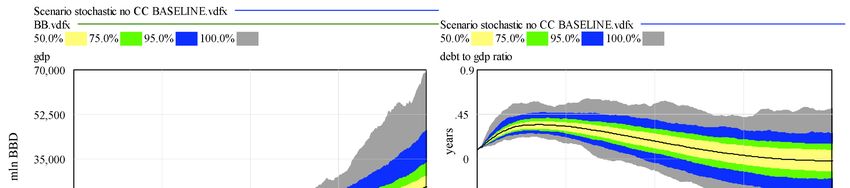
Economies 2020, 8, 16                                                                             2 of 21

or enhancing positive outcomes. This is, indeed, a well-established reason for building scenarios.
As Pierre Wack (1985), a scenario pioneer, wrote in a classic paper, “Scenarios serve two main purposes.
The first is protective: anticipating and understanding risk. The second is entrepreneurial: discovering
strategic options of which you were previously unaware.” The robust decision-making strategy will
also be familiar to policy makers in SIDS. Demas (2009; originally published in 1965) argued that one
of the advantages of small size is “greater flexibility”, a point also made by Kuznets (1960), and SIDS
deploy a variety of strategies and tactics to respond to external events.
     The model presented in this paper combines an updated version of a macroeconomic model
for Caribbean states (Kemp-Benedict et al. 2018), a model of storm damage to capital stocks for
Barbados (Kemp-Benedict et al. 2019), and a tourism sector model based on an empirical model by
Laframboise et al. (2014). To these, we added sub-models developed in this paper for global GDP
growth, economic growth in tourism source markets, and payouts from the Caribbean Catastrophic
Risk Insurance Facility (CCRIF).
     The economic model follows the structuralist tradition in development economics. That tradition,
which arguably grew from Rosenstein-Rodan’s (1943) classic paper, had a strong influence on
development thinking (Chenery 1975). It dominated Caribbean economic thought for decades through
the work of Sir Arthur Lewis (1954), Demas (2009), Best (1968), and Girvan (2006), among others.
The stream of structuralism applied in this paper, which is compatible with Caribbean structuralism,
is today developed and promoted by economists such as Lance Taylor, Jose Ocampo, Luis Carlos
Bresser-Pereira, and their collaborators (Taylor 1989; Ocampo et al. 2009; Bresser-Pereira et al. 2015).
Structuralist models in this stream are demand-led, with firms investing in anticipation of future
demand, while saving and the trade balance accommodate. Demand-led models are particularly
appropriate for SIDS, where the domestic economy is strongly reliant on the export sector, which
drives the rest of the economy through a multiplier process. The “structure” of structuralism refers
both to productive structure of the economy as well social and institutional structures in which the
economy is embedded (Gibson 2003; Ocampo et al. 2009).
     The structuralism of Taylor and others can be contrasted with the neoclassical “new structural
economics” (Lin 2012). The new structural economics is concerned with the balance between the
role of public and private actors in the economy, criticizing the “old structuralism” for its focus on
public investment and planning. It emphasizes the role of markets in resource allocation, with the
state playing a coordinating or facilitating role. The “structure” in new structural economics is the
prevailing structure of factor endowments. While the new structural economics offers some potentially
useful techniques, such as the “growth diagnostics” method of Hausmann et al. (2008), it tends to take
the neoclassical conception of the market as given. Indeed, Hausmann et al. (2008, p. 327) claim that
an economy that is underperforming and in need of reform is “by definition” plagued with market
imperfections and distortions. As noted by Felipe et al. (2008), while the growth diagnostics approach
might be useful in some situations, its scope is severely limited and must be applied cautiously.
More broadly, the central analytical task of the new structural economics is to determine how the
endowment structure must change in order to promote growth (Lin 2012, p. 99). Such a study can
provide insight when preparing a development strategy, but from the perspective of Taylor, Ocampo,
and Bresser-Pereira’s structuralism, it is quite narrow and begs the question of what drives changes in
the endowment structure.
     The structuralist approach in this paper can be further contrasted with the balance-of-payments
constrained growth theory of Thirlwall (1979, 2011). Cimoli and Porcile (2014) showed that Thirlwall’s
model can be combined with the Kaldor-Verdoorn law and a Lewis-type subsistence labor model to
generate a useful North–South model along structuralist lines. The model presented in this paper is
not inconsistent with balance-of-payments constrained growth, but it views long-run trajectories as
emerging from short-run dynamics. We therefore do not impose the balance of payments constraint
but rather allow it to emerge as a tendency.
Economies 2020, 8, 16 3 of 21
We constructed a simulation model, which Gibson (2003) argues is a technique well suited to
structuralist theory. We then ran the model using a mix of Monte Carlo and scenario approaches
in keeping with the RDM methodology. In the terminology of Knight (1921), we considered some
uncertainties to be quantifiable risks, while others were fundamental uncertainties. For the former,
such as global GDP growth, we provided a stochastic model and ran it in Monte Carlo mode, drawing
parameter values from a probability distribution. For the latter, such as future sea-surface temperature,
we could not provide a stochastic model, and instead allowed for distinct alternatives. Once sea-surface
temperature was given, we ran a stochastic model of storm damage, but the parameters themselves
depended on a cascading set of uncertainties, some of them irreducible to probabilistic calculations
(Collins et al. 2013).
While the model is in development, initial results show that, even in the absence of climate change,
fluctuations in export and tourism demand within historical bounds can lead to substantially different
GDP and external debt trajectories. Such changes are largely out of the control of Barbadian authorities,
thus there is need for robust strategies and policies to manage the impact of those fluctuations on the
economy. Under a climate change scenario, it becomes even more challenging to manage external debt
due to rebuilding costs, loss of productive capital, and the resulting increase in imports.
1.1. The Barbados Economy
The post-independence period of the Barbados economy is characterized by succeeding periods
of growth and contraction. In the 1960s and the 1970s, annual average economic growth was 5%.
During this period, the economy was driven primarily by agricultural production, particularly sugar
cane. By 1980, the economy had diversified, with agriculture accounting for 9% of GDP, wholesale
and retail trade 17%, general services 14%, manufacturing to 12%, and government services and
tourism to 11% each. The economy in the 1980s was negatively impacted by the global recession,
but by 1986, the economy again grew by 5% each year due to strong performances in the foreign
exchange earning sectors of agriculture, tourism, and manufacturing (Meditz and Hanratty 1987).
In the early 1990s, the economy again was impacted by the external economic environment and entered
an International Monetary Fund (IMF) program that sought to deliver balance of payment support. By
1993, the economy was recovering and continued to grow during the 1990s, driven by tourism and
construction sectors.1
The post 2008 global recession period brought low or no growth to the small island economy.
From 2008 to 2018, the annual average GDP growth rate was 0.1% (using data from the World Bank
WDI and Central Bank of Barbados 2018). Further, the country’s external debt increased to 150% of
GDP, contributing to a fiscal deficit of 5% of GDP in 2016 (Central Bank of Barbados 2018). This led to a
sovereign debt default and the country signing onto a four year IMF Extended Fund Facility in 2018.
Barbados’ economy is heavily reliant on the tourism sector. Tourism directly accounts for 13%
of GDP and indirectly for 40%. The sector also supports, directly and indirectly, around 40% of total
employment on the island (WTTC 2018). The tourism sector is the main foreign exchange earner, and
in June 2019, it recorded 3.9% growth while all other sectors had contracted. This increase was due to
increases in arrivals from the United Kingdom and the United States. However, cruise tourism fell by
1.9% due to rerouting of itineraries to original ports following disruptions form the 2017 hurricane
season (Central Bank of Barbados 2019). Given the island’s dependence on tourism for economic
activity, the impacts of climate change—including stronger, more frequent hurricanes (Granvorka
and Strobl 2013), sea level rise (Scott et al. 2012), loss of coral reefs (Burke and Maidens 2004), and
increasing droughts (Cashman and Nagdee 2017)—have direct implications for the sector (Moore 2010;
ECLAC 2011; Cashman et al. 2012). Because of the sector’s economic importance, climate change holds
1 https://thecommonwealth.org/our-member-countries/barbados/economy.Economies 2020, 8, 16 4 of 21
indirect implications for the entire economy. This is true for many Caribbean countries, as the region is
the most tourism dependent in the world (Thomas 2015).
Barbados has played an active and prominent role in regional integration, being a founding
member in 1973 of the Caribbean Community and Common Market (CARICOM). Barbados maintains
a Cabinet position within CARICOM. In addition, through the Revised Treaty of Chaguaramas in 2001,
Barbados led the establishment and the implementation of the CARICOM Single Market and Economy
(CSME) up until 2008. Among its various benefits, the CSME allows its members the free movement of
goods and services, the right of establishment, an external common tariff, and the free movement of
capital and labor.
1.2. Barbados in a Changing Climate
Barbados is on the southern edge of the hurricane belt, thus most years it suffers little
damage from tropical cyclones. Nevertheless, it is periodically struck, sometimes severely.
Kemp-Benedict et al. (2019) estimate a strike probability for Barbados of just over one-third for
storms in the Eastern Caribbean.
Climate models exhibit low skill in projecting tropical cyclone frequency and intensity
(Nurse et al. 2014, p. 1634), and give ambiguous results for Atlantic tropical storms (Villarini and
Vecchi 2012). With extremely wide variation, the trend is towards an increasing number of tropical
storms through 2050, with no change beyond that. In this paper, we use a model developed by
Kemp-Benedict et al. (2019) that relates storm intensity and frequency in the Eastern Caribbean to
changes in sea-surface temperature (SST). In contrast to projections of tropical cyclones, climate models
unambiguously suggest rising SST, whether at global scale, in the tropics, or in the North Atlantic
(Villarini and Vecchi 2012). Given the uncertain results on tropical cyclones from climate models,
the model accepts a range of parameter values to allow for different climate scenarios.
1.3. The Caribbean Catastrophic Risk Insurance Facility (CCRIF)
The Caribbean Catastrophic Risk Insurance Facility (CCRIF) Segregated Portfolio Company
(SPC) is a regional catastrophic risk pool mechanism. It was established in 2007 in response to
the damage from hurricane Ivan in 2004. The purpose of the CCRIF is to cover damage to public
infrastructure, whereas the focus for the model described in this paper is damage to private physical
capital. As described below, the role of the CCRIF sub-model in our simulation model is to offset the
need for external borrowing after a storm.
The CCRIF offers parametric insurance—that is, insurance following a trigger event rather than
after an assessment of loss—for states in the Caribbean and, since 2015, Central America. This feature
facilitates its inclusion in the present model, because it allows us to use simulated peak wind speeds as
the parameter for the simulated payout. The payout model is described in a later section.
As with other risk pools, the aim of the facility is to support a group of countries facing a common
risk with at least partially independent probabilities of loss. Compared with a conventional approach
in which each country purchases insurance independently, the CCRIF SPC risk pool reduces countries’
premium costs by up to half of what they might pay on their own (CCRIF 2018a).
Insurance products offered by CCRIF SPC are classified as both parametric, as defined above, and
sovereign. The triggering events for the parametric insurance include tropical cyclones, earthquakes,
and excess rainfall. The insurance is sovereign because the policy owners are the governments of
the contributing states, and the insurance is meant to protect government budgets from disaster
impacts. The CCRIF SPC offers coverage for losses caused by wind and storm surge caused by
tropical cyclones (for one-in-10-years events), and by excess rainfall (from one-in-15-years events)
(Martinez-Diaz et al. 2019).
Barbados is a loyal customer of CCRIF SPC (Martinez-Diaz et al. 2019). It has purchased insurance
products from CCRIF SPC every year and has been covered against tropical cyclones and earthquakes
since 2007 and excess rainfall since 2014. Barbados is also the country that has received the higherEconomies 2020, 8, 16 5 of 21
number of payouts (six out of 38 payouts from 2007 until 2018), all from tropical cyclones and excess
rainfall events, receiving a total of US$ 19.3 million (CCRIF 2018b). All payouts to Barbados have
gone from the CCRIF SPC to Barbados’ Consolidated Fund within 14 days after the event, providing
liquidity to the governments and allowing them to respond quickly. Payouts have been administered
by the Ministry of Public Works and used mainly for immediate post-event activities, including the
repairing of public infrastructure such as roads and bridges and remedial work in low lying areas
(CCRIF 2018b). The funds are intended to cover immediate needs only, not all recovery-related costs.
Thus, the size of the payouts is relatively small in comparison to the damage caused by covered events.
1.4. Exchange Rate Management in Barbados
Barbados has adopted a fiscal strategy for countering the depletion of foreign reserves, which are
chronic in small open economies (Worrell et al. 2003). That system has allowed the country to maintain
its exchange rate peg at 2 BBD/USD since 1975, despite periodic pressures on foreign reserves. In this
system, the central bank and the Ministry of Finance use a forecasting model to identify a target level
for the fiscal balance consistent with the target exchange rate. Given the target, the Finance Ministry
engages with spending ministries to decide how to achieve it. Adjustment may include both increased
taxes and decreased government spending in order to increase domestic saving, requiring flexibility
and acquiescence from both citizens and ministries. During a balance of payments crisis that began in
1991, Barbados expanded the system, establishing a body to oversee the process, the Joint Economic
Group (JEG), and negotiating a “tripartite accord” with labor on wages, prices, and productivity.
For the purposes of the model presented in this paper, we do not seek to represent this complex
process in any detail. Rather, we represent the outcome by relying on accounting relationships and a
simple behavioral rule.
We begin with a standard economic balance, equating injections into the economy—purchases
of consumption and investment goods C and I, income from exports, X, government expenditure,
G, incoming personal remittances R, and payouts from the CCRIF Fpay —to their corresponding
leakages—consumption expenditure (also equal to C), saving S, imports M, taxes T, remitted profits
Πr , and premium payments to the CCRIF Fprem . In this section, we express all variables in nominal
terms, thus the balance is
C + I + X + G + R + Fpay = C + S + M + T + Πr + Fprem . (1)
| {z } | {z }
injections leakages
Consumer goods C enter on both the injection and the leakage sides of the equation and cancel
out; the textbook result. In Barbados as well as other small island economies, there is little capacity to
produce investment goods, and we assume that all are imported. Imports then consist of investment
goods I, imported consumption goods Mc , and intermediate imports for domestic production, Mi .
With these definitions, and rearranging to solve for imports of consumption goods, we can rewrite
Equation (1) as
Mc = X − Mi − (S + T − G) + R − Πr + Fpay − Fprem . (2)
| {z } | {z } | {z }
total domestic net remittance net CCRIF payout
saving inflows
Most of the terms on the right-hand side of this equation are fully determined in the model.
Exports are determined by global demand; intermediate imports by domestic production; remittance
inflows from citizens or relatives living abroad by a factor applied to GDP; and remittance outflows to
meet contractual obligations or remit profits by a factor applied to the capital stock. The remaining
term is total domestic saving.Economies 2020, 8, 16 6 of 21
To determine a rule for total domestic saving, we note that, while in principle, foreign savings
can complement domestic savings, in practice, they tend to substitute for them (Bresser-Pereira et al.
2015, chp. 8). The mechanism operates through the exchange rate. Capital inflows represent a demand
for the domestic currency, which causes it to appreciate, other things remaining equal. That drives
wages and imports of consumption goods upward. The rising wage squeezes profits, which are only
partially offset by the fall in the cost of intermediate imports. That depresses savings, and the balance
of payments worsens.
Barbados’ strategy offsets the potential crowding out of domestic private savings by increasing
public saving through the fiscal balance. For the purposes of the present model, where we do not
explicitly represent government spending, we express this rule through a target domestic saving rate
sd targ , which is then multiplied by GDP, Y, giving an expression for imports of consumer goods Mc .
This gives an upper bound for the level of imports of consumer goods,
targ
Mc ≤ X − Mi − sd Y + R − Πr + Fpay − Fprem . (3)
This constraint is maintained by adjusting the saving rate. It is possible for the right-hand side to
become negative, in which case the upper bound is set to zero.
Fiscal mechanisms operate slowly, thus the balance in Equation (3) may not be achieved in
any given time period. Rather, realized domestic savings will fluctuate around the target level.
The implementation in the model is described below in Section 2: Methodology.
2. Methodology
As noted in the Introduction, the core of the model presented in this paper is a macroeconomic
simulation model built along structuralist lines (Taylor 1989; Ocampo et al. 2009; Bresser-Pereira 2012).
The model is documented in a separate paper (Kemp-Benedict et al. 2018). While we leave the details
to that paper, we briefly describe the structure and the main assumptions below. Data requirements
are summarized in the Appendix A.
2.1. Dynamic Macroeconomic Model
The main calculations underlying the economic model are shown in Figure 1. Consumption both
fuels and is driven by GDP. Some of that consumption is in the form of imports, which are balanced
against exports (net of remittances) to determine the change in the external debt. Trend GDP growth
sets longer-run expectations for firms. In the short run, GDP growth in excess of growth in the capital
stock indicates rising capital utilization and is taken by firms as a sign of rising demand and therefore
a stimulus to investment. However, because investment goods are imported, investment expenditure
contributes to the external debt.2 That is assumed to increase the perceived risk of investment in the
country by external investors, thus further investment is dampened when the debt-to-GDP ratio rises.
Once investment is determined, it contributes to the capital stock.
2 While capital goods are largely imported, investment expenditure also includes domestic construction. We plan to include
this in future iterations of the model.sets longer-run expectations for firms. In the short run, GDP growth in excess of growth in the capital
stock indicates rising capital utilization and is taken by firms as a sign of rising demand and therefore
a stimulus to investment. However, because investment goods are imported, investment expenditure
contributes to the external debt.2 That is assumed to increase the perceived risk of investment in the
country2020,
Economies by external
8, 16 investors, thus further investment is dampened when the debt-to-GDP ratio7rises.
of 21
Once investment is determined, it contributes to the capital stock.
GDP utilization
consumption
GDP growth
exports investment capital
remittances debt-to-GDP
debt
imports
Figure 1. Flow of calculation in the core macroeconomic model (from Kemp-Benedict et al. 2018).
Figure 1. Flow of calculation in the core macroeconomic model (from Kemp-Benedict et al. 2018).
At the highest level of abstraction, domestic economic activity in the model results from a
At the
multiplier highest
applied level of While
to exports. abstraction, domestic
this is similar economic
to “export base”activity
theoryin the model
(North resultsenjoyed
1955), which from a
multiplier
some applied
popularity in to
theexports.
1970s, the While this is in
multiplier similar to “export
the model base” rather
is dynamic theorythan(North 1955),
static, as itwhich
is in
enjoyed some popularity in the 1970s, the multiplier in the model is dynamic rather
export base models (Lewis 1976). The dynamic multiplier is constructed by starting with a two-sector than static, as it
is in export base models and
model—export-oriented (W. C. Lewis 1976). The
domestic—and dynamic
through multiplier is constructed
an input–output type analysis, by starting
derivingwithan
a two-sector
effective model—export-oriented
one-sector model with the two-sector and domestic—and
model parameters through
and an input–output
exogenous prices type analysis,
embedded in
deriving an effective one-sector model
it. The approach was inspired by the work of with the two-sector model parameters and exogenous
Caribbean structuralists Seers (1964) and Bruce and prices
embedded
Girvan in who
(1972), it. The approach
carried out awas inspired
similar by thefor
calculation work
the of the Caribbean
special structuralists
case of a petroleum Seers Aside
exporter. (1964)
and Bruce
from and Girvan
the intuitive appeal(1972),
of thewho carried the
multiplier, outattraction
a similar calculation
of this typefor the special
of model case
is that of a petroleum
output variables
are at the level of the whole economy rather than the two sectors, which facilitates calibration when
2
data While capital goods are largely imported, investment expenditure also includes domestic construction. We
are scarce.
plan to include this in
The assumption of future iterations
exogenous of the
prices model. some justification. For small open economies, it
requires
is plausible to assume exogenous prices for tradeable goods. Yet, the same also appears to hold for
non-tradeables. Holder and Worrell (1985) found, in a study that included Barbados, that the price
of tradeables had a much stronger effect than either wage rates or bank lending rates on the price
of non-tradeables.
In the model runs reported in this paper, we held structural parameters fixed at their calibrated
values, thus changes in the multiplier are driven by relative price changes. In scenario exercises, it is
possible to change structural parameters exogenously to allow for greater or lesser integration between
the domestic and the export sectors, changing import propensity, different sector wage shares, and
so on.
The model is implemented as a system dynamics model implemented in the modeling software
Vensim DSS.3 The model economy is normally out of equilibrium. As a structuralist model, it is
demand driven; when demands depart from expectations, economic actors are assumed to act only
after a delay. In economic modeling, this is normally referred to as adjustment following a shock.
However, as the economy is strongly dependent on fluctuating external demand and climate events, it
is effectively always being “shocked”. Admittedly, some of those shocks—such as global recessions or
severe storms—are unusually large, a possibility that we incorporate into the model.
In this paper, we make four significant extensions to the model as documented in Kemp-Benedict
et al. (2018). First, as described in the introduction, we simulate the outcome of the exchange rate
management regime. Second, we construct a model for global GDP growth in order to drive export
demand. Third, we construct a separate model for the tourism sector. Fourth, we apply a model for
payouts from the CCRIF SCP.
3 The model code is available at: https://github.com/sei-international/SIDS_climate_economy_model_BB.git.Economies 2020, 8, 16 8 of 21
2.2. The Exchange Rate Management Regime
Our strategy for simulating Barbados’ fiscal exchange rate management regime was described in
the Introduction. We now say explicitly how it is implemented in the model. We first put Equation (3)
in terms of real variables by explicitly giving prices,
targ
h i
Mmax
c = max 0, eP∗x X − eP∗m Mi − sd PY + R − Πr + Fpay − Fprem . (4)
In this expression, e is the exchange rate, P is the general price level, Px and Pm are the prices of exports
and imports, and a star indicates a world price, denominated in US dollars.
Imports of consumption goods are a fraction of consumption above a basic level. Basic
consumption, which is a fixed multiple c0 of the population, N, is assumed to be fully supplied
by domestic producers at a price Pd . Households target a desired level of saving sw desired with a
(price-dependent) import fraction m. They then devote a fraction of their smoothed wage income W in
excess of basic consumption to desired imports of consumer goods,
Mdesired
c = m 1 − sdesired
w (W − Pd c0 N ). (5)
If this exceeds the maximum level of imports consistent with the target saving rate, then the Central
Bank and the Finance Ministry will intervene in order to raise total saving. In the model, this
intervention is represented by a target level of consumer goods imports,
targ
Mc = min Mmax
c , Mdesired
c , (6)
which corresponds to a target saving rate,
targ
Mtarg
c
sw = 1 − 1 − sdesired
w . (7)
Mdesired
c
Because this is achieved through a fiscal mechanism and therefore operates after a delay, we assume
that the actual saving rate tracks the target with a one-year smoothing time.
2.3. Demand Drivers
In this demand-led model, the main external sources of demand are for goods and services exports
and domestic expenditure by tourists. We treat tourist revenue as export demand, although that
demand is realized by in-country payments.
Income in tourist source countries is an explanatory factor for tourist arrivals (Moore 2010). Due
to global economic conditions, we expect the source countries’ GDP to move together to some degree.
Similarly, we expect changes in export demand to reflect global economic conditions. To generate
consistent external demand scenarios, we constructed a model for the world GDP growth rate, gw ,
and used it as an explanatory variable for growth rates of export demand and income in tourist
source countries.
Attempting an autoregression using data from the World Bank World Development Indicators
for 1980–2018 yielded residuals that deviated strongly from normality due to the global recessions in
the early 1980s, the early 1990s, the early 2000s, and the Global Financial Crisis (p = 0.013 with the
Shapiro–Wilk test). We therefore represented the world GDP growth rate by separating recessions
from normal conditions. We used an autoregressive model for normal conditions and a mixed
Poisson-exponential model for recessions. We constructed a modified time series by setting the
world growth rates in 1982, 1991, 2001, and 2009 to 3.15%/year, which is the mean value with those
years removed. Carrying out the autoregression in R using the Yule-Walker algorithm and choosing
the optimal order using the Akaike Information Criterion (AIC) measure gave an order one model.
The residuals for the modified time series were acceptably normal (p = 0.865 with the Shapiro–Wilk test).Economies 2020, 8, 16 9 of 21
We modeled the occurrence of recessions as a Poisson process with an annual probability of recession
of 10% (four recessions over 39 years) and the depth of the recession as a truncated exponentially
distributed variable with a mean depth below trend of 2.6%/year and a maximum depth of 10.0%/year.
Most tourists to Barbados arrive from the UK (over 35%), the US (about 25%), other CARICOM
countries (about 15%), and Canada (about 12%). We assume all tourists come from these four source
markets. For the model runs in this paper, we represent CARICOM by the World Bank’s “Caribbean
Small States” group (CSS).4 For each country and the CSS, we modeled the GDP growth rate of source
country or region s as a stochastic process,
gs = as0 + as1 gs,−1 + bs0 gw + bs1 gw,−1 + σs B. (8)
In this equation, σs is the standard deviation of the residuals of the fitted model, and B is a standardized
normal random variate. The model structure is a compromise. For each of the three countries (UK, US,
and Canada), each coefficient (aside from the constant) is significant at least at the 10% level. For the
CSS group, the coefficient on the lagged world GDP growth rate is not significant but is retained to
maintain the same structure across tourism source markets. Given the non-normality of the residuals
for world GDP, we ran the Shapiro–Wilk test as a check, which gave acceptable results (US: p = 0.208;
UK: p = 0.838; Canada: p = 0.157; CSS: p = 0.340).
For the growth rate of export demand (excluding tourism revenue), we found that it can be
reasonably modeled as depending solely on the instantaneous value of the world GDP growth rate.
The constant term was insignificant and small, thus we ran the regression with the intercept set to zero.
Using a notation similar to that above, the export growth model is,
gX = bX0 gw + σX B. (9)
The coefficient bX0 is very nearly equal to one (0.943), thus trend growth in demand for Barabados’
exports follows growth in the global economy very closely. However, the deviations are large, with
σX = 9.7%/year. The Shapiro–Wilk test statistic for the residuals is consistent with normality (p = 0.877).
2.4. The Tourism Sector
Tourist revenue is calculated for tourist season, which is taken to be the first quarter of each
year. As noted earlier, the revenue is treated as part of exports. A number of tourism models are
available, including ones by Moore (2010) and Laframboise et al. (2014). Moore makes use of a tourism
climate index (TCI) proposed by Mieczkowski (1985). This is a compelling approach, because climate
indices, whether TCI or more recent alternatives (de Freitas et al. 2008; Mailly et al. 2014), include
climate-related variables that can be drawn from climate models. Moreover, local indices can in
some cases be computed from indices at coarser resolution using statistical downscaling techniques
(Casanueva et al. 2014). However, aside from unresolved challenges in making long-run projections of
climate tourism indices (Dubois et al. 2016), implementing a climate index would require a finer time
resolution than the quarterly time step we assumed in our model. We therefore adopted one of the
models tested by Laframboise et al. (2014). Specifically, we chose the model for tourism expenditure
in which tourism-weighted GDP per capita is the income proxy (Table II.2 in Laframboise et al.). We
depart from that paper, however, by using the tourism-weighted GDP growth rate rather than GDP
per capita.
4 The CSS countries include Antigua and Barbuda, Bahamas, Barbados, Belize, Dominica, Grenada, Guyana, Jamaica, St. Kitts
and Nevis, St. Lucia, St. Vincent and the Grenadines, Suriname, and Trinidad and Tobago. About 10% of all visitors to
Barbados were from Trinidad and Tobago alone. In CARICOM, but not in CSS (and therefore excluded from the parameter
estimates) are Haiti and Montserrat.Economies 2020, 8, 16 10 of 21
Besides tourism-weighted GDP growth in source markets gsource , the model of Laframboise et al.
(2014) depends on a hurricane dummy, h, the tourism-weighted real exchange rate esource , and the
number of airlines serving Barbados, A. Using a “hat” to indicate a growth rate and denoting tourist
income by Xtour , the model is,
X̂tour = c1 gsource − c2 h − c3 esource + c4 Â. (10)
Of these variables, gsource is computed using the model described in the previous section, esource is
computed using an exogenously specified exchange rate e, the computed price level in Barbados, and
price indices in source countries, and A is given exogenously. The hurricane dummy h is computed
using a storm damage model documented in Kemp-Benedict et al. (2019), as described in the next
section.
2.5. Climate Impacts
The storm damage model of Kemp-Benedict et al. (2019) simulates hurricane events by running
the simulation model in Monte Carlo mode using a probabilistic model. Because hurricanes in Barbados
are comparatively rare, hurricane arrivals in Barbados are computed as a strike probability (estimated
to be 36%) multiplied by the probability of arrival in the Eastern Caribbean as a whole, which is
represented by a generalized extreme value (GEV) distribution. Peak wind speed in a given year is
treated as an independent draw from the distribution, which is characterized by location, scale, and
shape parameters. Historically, the peak wind speed recorded in Barbados has been on average about
three quarters of the peak wind speed for the Eastern Caribbean as a whole, thus after fitting the GEV
to data for the Eastern Caribbean, we adjusted the location and the scale parameters by that factor.
Under climate change, the distribution of storm arrivals and intensities is not stationary, thus the
parameter values of the GEV distribution are expected to change. Testing a nonstationary model with
global sea-surface temperature (SST) as a covariate showed a significant relationship for the location
parameter. In the simulation models, climate scenarios are therefore specified by a trajectory for SST,
which drives the location parameter in the GEV, thereby driving up average peak wind speed.
The original model was built for annual hurricane events and was run at a yearly time step. In the
model described in this paper, which is run at a quarterly time step, hurricanes appear only during
“hurricane season”, which is taken to be the third quarter of each year. Firms anticipate climate damage
when they make new investments, balancing current adaptation expenditures against future rebuilding
costs. They do this in a typical engineering cost-minimization exercise that compares capitalized
investment expenditure to discounted expected damages. However, they may not correctly anticipate
future climate. In this paper, we assume that they do not, and continue to assume historical climate
when making new investments.5
The climate damage model applied in this paper is inspired by the treatment of extreme events
in engineering studies, where the aim is to build infrastructure that can withstand all but the
most infrequent and damaging events. Under stationary conditions, a popular parameter is the
return period. Under nonstationary conditions, the concept of a return period becomes problematic
(Read and Vogel 2015). Nevertheless, given its intuitive appeal, changes in return period were used
in the IPCC Special Report on Extreme Events (SREX) to illustrate the impacts of climate change
(IPCC and Field 2012). This engineering approach can be contrasted with the highly aggregate “damage
function” approach used in some prominent integrated assessment models (IAMs), such as DICE
(Nordhaus 1993, 2017) and FUND (Anthoff and Tol 2012). In such models, greenhouse gas concentration
in the atmosphere or global temperature determines economic losses. Losses are typically given as a
fraction of GDP, although in some cases they represent loss of fixed capital (Fankhauser and Tol 2005;
5 See Kemp-Benedict et al. (2019) for the consequences of anticipating climate change.Economies 2020, 8, 16 11 of 21
Rezai et al. 2013; Piontek et al. 2018). In the model described in this paper, we used global sea surface
temperature to compute a (stochastic) peak wind speed, which then determines losses to capital stocks
of different vintages. Thus, the overall logic is the same as in the IAMs—a global climate parameter
drives economic losses—but we simulated the decision process and used a physically-motivated storm
model to calculate damages.
While we did not explicitly consider public infrastructure, we did take into account the impact
of CCRIF premiums and payouts on the current account. We assumed a series of fixed premium
payments in US dollars. Following a World Bank (2007) background document to the creation of the
CCRIF, we simulated payouts as rising from zero below an “attachment” wind speed and plateauing
at a maximum payout Fpay max above an “exhaustion” wind speed. For the simulations, we chose the
attachment wind speed to be the lower limit for a tropical storm, wTS , and the exhaustion wind speed
to be the lower limit for a category five hurricane, wCAT5 . Between those limits, the payout increased
as the fractional distance between the attachment and the exhaustion wind speeds raised to the power
of a damage exponent β. That is,
0, w < wTS
max w−wTS β
Fpay = Fpay w , wTS ≤ w < wCAT5 (11)
CAT5 −wTS
Fmax ,
w ≥ wCAT5
pay
We note that, because the CCRIF only covers damage to public infrastructure, it is not a large correction
to total damage expenditure in the model.
We further took into account loss in global GDP due to climate change using the damage
function from the DICE integrated assessment model. The effects were essentially negligible, which
might not have been the case if the damage function allowed for a higher probability of catastrophic
damage (Weitzman 2009, 2011; Ackerman and Stanton 2012). The DICE damage function depends
on atmospheric temperature rather than SST. Following historical patterns based on ordinary least
squares (OLS) regression of the global temperature anomaly on the SST anomaly using data from
National Oceanic and Atmospheric Administration (NOAA), we found that the annual rise in global
temperatures is about 12.5% higher than the annual rise in SST. We applied that dependence to our SST
assumption and used the damage function from DICE-2016R (Nordhaus 2017).
3. Results
In this section, we present some key results from runs of the model. We ran the model to 2080,
a common choice for a future year in climate scenario projections. We ran two scenarios, one with
a historical climate and the second with a warming climate. We ran the model under each scenario
1000 times, using the same pseudo-random number sequence in each case.
First, we consider the scenario without climate change. Key economic variables are shown in
Figure 2. As shown in the figure, in the average case, GDP rises in line with historical rates but with the
possibility of much slower or faster growth depending on global economic conditions and variability in
export demand. The debt-to-GDP ratio initially rises in all variants, as in Kemp-Benedict et al. (2018).
However, it subsequently declines—without triggering the exchange rate stabilization mechanism—to
gradually return close to zero in the average case.2 BlueGreen Initiative Inc., Peterkin Road, Bank Hall, St. Michael, Bridgetown BB11059, Barbados;
crystal@bgibb.com
3 Stockholm Environment Institute (SEI Latinoamérica), Calle 71, #11-10, Edificio Corecol, Oficina 801,
Bogotá, Colombia; nella.canales@sei.org
* Correspondence:
Economies 2020, 8, 16 eric.kemp-benedict@sei.org; Tel.: +1-617-590-5436 12 of 21
Received: 22 December 2019; Accepted: 21 February 2020; Published: 25 February 2020
0
Article
AFigure
Climate-Economy
2. GDP and debt-to-GDP ratio in Policy Model
the scenario without climatefor Barbados
change (probability bands for
Abstract:
1000 runs). Small island developing states (SIDS), such as Barbados, must continually adapt in the
Eric Kemp-Benedict
face of uncertain
1 Stockholm
1,*, Crystal Drakes 2 and Nella Canales 3
external drivers. These include demand for exports, tourism demand, and extreme
Environment Institute, Somerville, MA 02144, USA
In the baseline
2 weather events.scenario,
Climate we assume
change that the global
introduces further trends from 1985
uncertainty into tothethe present
external continue
drivers. To into
address
BlueGreen Initiative Inc., Peterkin Road, Bank Hall, St. Michael, Bridgetown BB11059, Barbados;
the future.
the This leads
challenge, weto a steady
present a mean growth
policy-oriented rate of about
simulation 3%/year,
model as
that shown
builds in Figure
upon 3.
prior However,
work by the
crystal@bgibb.com
the growth
3 authorsdistribution
andEnvironment
Stockholm is decidedly
their collaborators. asymmetric
Intended
Institute (SEI because
for policy
Latinoamérica), of the Poisson-exponential
analysis,
Calle it follows
71, #11-10, recession
a robustOficina
Edificio Corecol, model.
decision
801,making
Recessions
(RDM) arephilosophy
Bogotá, shown innella.canales@sei.org
Colombia; the
of second panelpolicies
identifying of Figure 3, where
that lead tothey are most
positive likely toacross
outcomes be absent or small
a wide range of
but may, in some
* external circumstances,
Correspondence:
changes. leadmodel
to a large
eric.kemp-benedict@sei.org;
While the canfall in+1-617-590-5436
Tel.: the global
benefit GDP growth
from further rate.
development, it illustrates the
importance for SIDS of incorporating climate change into national planning. Even without climate
change, normal variation in export and tourism demand drive divergent trajectories for the
economy and external debt. With climate change, increasing storm damage adds to external debt as
the loss of productive capital and need to rebuild drives imports.
0.
Keywords: SIDS; Caribbean; climate change; climate adaptation; tropical cyclone; parametric
insurance; tourism
JEL Classification: E12; E6; O21
Received:Figure
22 December
3. World2019;
GDPAccepted: 21 global
growth and February 2020; Published:
recessions 25 February
(probability bands for 2020
1000 runs).
1. Introduction
Selected model
Abstract: outputs
Small island for a single
developing model
states run, such
(SIDS), whichasincludes
Barbados, climate
must change,
continuallyare shown
adapt ininthe
Figure This paper
cost ofpresents an economic simulation model for in
thegraph
small(a).
island state of Barbados.time,With
face4.ofThe
uncertain climate damage
external drivers. rises
Theseover time,
include as shown
demand for exports, Rebuilding
tourism demand,takes
and extreme
a
leading focus on
to the the medium
sharpClimate to longer
rise andchange
the smoothrun future, the
decayfurther model seeks
of lossuncertainty
and damage to represent a
expenditure. set of uncertain
Rebuilding external
also
weather events. introduces into the external drivers. To address
factors
requires that can
imports ofwe significantly
capital goods, impactareupon
which economic
reflected in graphoutcomes.
(b). that These
Climate include demandwith
damage for the
the challenge, present a policy-oriented simulation model builds upon combined
prior work by the
country’s
fluctuations exports, tourism, and damage to capital stocks from tropical storms.
authors in andworld
theirGDP, shown in graph
collaborators. Intended(c), for
affect tourist
policy expenditure
analysis, in graph
it follows (d). The
a robust multiplier
decision making
effect(RDM) While
from export the model
demand is specific to
can be seen Barbados,
in graph many small island developing states (SIDS) face
upsimilar
philosophy of identifying policies that(e).
lead Astoshown
positivein outcomes
the graph,acrossexports makerange
a wide a of
largechallenges.
component
external
They
changes.
are highly
of GDP,While itdependent
but the is model
dominatedon export
can by anrevenue
benefit indirect and are therefore
component
from further that vulnerable
development, is driven byto export
trade risks
it illustrates the
(Streeten
demand 1993;
through Briguglio 1995;
a (dynamic) McGillivray
multiplier. Employmentet al. 2011).
in the Tourism is anandimportant sector; the World
importance for SIDS of incorporating climate change intoexport sector
national planning.demand for domestic
Even without climate
intermediate goods
change, 2020,
Economies normal8, 16;drives
variationthe in
domestic
export economy.
doi:10.3390/economies8010016and tourism Thedemand
assumption drivethat households
divergent decide their
trajectories for the
www.mdpi.com/journal/economies
consumption
economy and based on smoothed
external debt. With wage income
climate rather
change, than instantaneous
increasing storm damage wageaddsincome results
to external in as
debt
smaller variations in GDP than in export demand, while
the loss of productive capital and need to rebuild drives imports. basic consumption declines in importance as
wages grow. The gap between imports and exports drives external debt, which varies as a share of
GDP,Keywords:
as shown inSIDS;graphCaribbean;
(f). climate change; climate adaptation; tropical cyclone; parametric
insurance; tourism
JEL Classification: E12; E6; O21
1. Introduction
This paper presents an economic simulation model for the small island state of Barbados. With
a focus on the medium to longer run future, the model seeks to represent a set of uncertain external
factors that can significantly impact upon economic outcomes. These include demand for the
country’s exports, tourism, and damage to capital stocks from tropical storms.
While the model is specific to Barbados, many small island developing states (SIDS) face similarcomponent of GDP, but it is dominated by an indirect component that is driven by export demand
through a (dynamic) multiplier. Employment in the export sector and demand for domestic
intermediate goods drives the domestic economy. The assumption that households decide their
consumption based on smoothed wage income rather than instantaneous wage income results in
smaller variations in GDP than in export demand, while basic consumption declines in importance
Economies 2020, 8, 16 13 of 21
as wages grow. The gap between imports and exports drives external debt, which varies as a share
of GDP, as shown in graph (f).
(a) (b) nominal exports and nominal imports
mln BBD
%
(c) (d)
mln BBD
1/year
Components of GDP
(e) 200,000
(f)
150,000
mln BBD
years
100,000
50,000
0
2011 2023 2034 2046 2057 2069 2080
Time (Year)
gdp basic consumption direct : Scenario stochastic CC BASELINE.vdfx
gdp exports direct : Scenario stochastic CC BASELINE.vdfx
gdp indirect : Scenario stochastic CC BASELINE.vdfx
Figure 4. Selected outputs from a single run of the model under climate change. (a) Loss and damage
Figure 4. Selected outputs from a single run of the model under climate change. (a) Loss and damage
as a share of GDP. (b) Export and import volume in nominal terms. (c) Global GDP growth rate
as a share of GDP. (b) Export and import volume in nominal terms. (c) Global GDP growth rate (a
(a driver for export and tourism demand). (d) Tourist expenditure. (e) GDP, broken into: minimal
driver for export and tourism demand). (d) Tourist expenditure. (e) GDP, broken into: minimal
household consumption demand (“basic” consumption); exports; demand induced through the
household consumption demand (“basic” consumption); exports; demand induced through the
multiplier (“indirect” demand). (f) External debt-to-GDP ratio.
multiplier (“indirect” demand). (f) External debt-to-GDP ratio.
The effect of the storm damage model can be seen when comparing the scenario with climate
The effect of the storm damage model can be seen when comparing the scenario with climate
change to that without. Under climate change, rebuilding costs rise substantially, as shown in Figure 5.
change to that without. Under climate change, rebuilding costs rise substantially, as shown in Figure
The 5.
saw-tooth pattern
The saw-tooth in the
pattern in figure arises
the figure from
arises hurricane
from damage
hurricane damageoccurring
occurringduring
during the hurricane
the hurricane
season, while, as noted above, rebuilding takes time.
season, while, as noted above, rebuilding takes time.Economies 2020, 8, 16 13 of 20
Economies 2020, 8, 16 14 of 21
Economies 2020, 8, 16 13 of 20
Economies 2020, 8, 16 13 of 20
Scenario stochastic no CC BASELINE.vdfx Scenario stochastic CC BASELINE.vdfx
50.0% 75.0% no CC95.0% 100.0% 50.0% 75.0% CC BASELINE.vdfx
Scenario stochastic 95.0% 100.0%
Scenario stochastic BASELINE.vdfx
loss
50.0%and damage
Scenario 75.0%as share
stochastic of GDP
no 95.0%
CC 100.0%
BASELINE.vdfx loss
50.0%and damage
Scenario 75.0%as share
stochastic ofBASELINE.vdfx
GDP
CC95.0% 100.0%
20.12
50.0% 20.12
50.0%
and damage75.0%
as share of 95.0% 100.0%
loss and damage75.0%
as share of 95.0%
GDP 100.0% loss GDP
loss and damage as share of GDP
20.12 loss and damage as share of GDP
20.12
20.12 20.12
15.09 15.09
15.09 15.09
% %
% %
15.09 15.09
10.06 10.06
%
%
10.06 10.06
10.06 10.06
5.03 5.03
5.03 5.03
5.03 5.03
0 0
2011 2028 2046 2063 2080 2011 2028 2046 2063 2080
0 0 Time (Year)
2011 2028 Time (Year)
2046 2063 2080 2011 2028 2046 2063 2080
0 0
2011 2028 Time (Year)
2046 2063 2080 2011 2028 Time (Year)
2046 2063 2080
Time (Year) Time (Year)
Figure 5. Rebuilding costs as a share of GDP.
Figure 5. Rebuilding costs as a share of GDP.
Figure5.5.Rebuilding
Figure Rebuildingcosts
costsasasa ashare
shareofofGDP.
GDP.
As storm damage increases, payouts from the CCRIF also increase, as shown in Figure 6. The
As storm
As damage increases, payouts from the CCRIFto also 20increase, as shown in Figure 6. 95%
The
Asstorm
average stormdamage
payout remains
damage increases,
well below
increases, payouts
the cap
payouts from the
(assumed
from the CCRIF
CCRIF also
bealso increase,
million
increase, asas
USD). shownin in
However,
shown Figure
the
Figure 6.
6. The
average
The payout
average
probability level remains
payout well
remains
eventually below
well below
exceeds the
the cap
the
cap. (assumed
cap (assumed to be
to be2020 million
millionUSD).
USD). However,
However, the
the 95%
95%
average payout remains well below the cap (assumed to be 20 million USD). However, the 95%
probability level
probability level eventually
eventually exceeds
exceeds the
thecap.
cap.
probability level eventually exceeds the cap.
Scenario stochastic no CC BASELINE.vdfx Scenario stochastic CC BASELINE.vdfx
50.0% 75.0% no CC95.0%
Scenario stochastic 100.0%
BASELINE.vdfx 50.0% 75.0% CC BASELINE.vdfx
95.0% 100.0%
Scenario stochastic
Scenario
50.0%
CCRIF stochastic
75.0% no 95.0%
payout CC BASELINE.vdfx
100.0% Scenario
50.0%
CCRIF stochastic
75.0% CC95.0%
payout BASELINE.vdfx
100.0%
50.0%
20 payout 75.0%
CCRIF 95.0% 100.0% 50.0%
20 payout 75.0% 95.0% 100.0%
CCRIF
CCRIF
20 payout CCRIF
20 payout
20 20
15 15
USD
USD
15 15
15
USD
USD
15
mlnmln
mlnmln
mln USD
mln USD
10 10
10 10
10 10
5 5
5 5
5 5
0 0
2011 2028 2046 2063 2080 2011 2028 2046 2063 2080
0 Time (Year) 0
2011 2028 2046 2063 2080 2011 2028 Time (Year)
2046 2063 2080
0 0
2011 2028 2046
Time (Year) 2063 2080 2011 2028 2046
Time (Year) 2063 2080
Time (Year) Time (Year)
Figure 6.
Figure 6. Caribbean
Caribbean Catastrophic
Catastrophic Risk
Risk Insurance
Insurance Facility
Facility (CCRIF)
(CCRIF) payouts.
payouts.
Figure 6. Caribbean Catastrophic Risk Insurance Facility (CCRIF) payouts.
Figure 6. Caribbean Catastrophic Risk Insurance Facility (CCRIF) payouts.
Due to the
Due the need
needto torebuild
rebuilddamaged
damagedcapital
capitalstocks, the
stocks, average
the external
average debt-to-GDP
external debt-to-GDP ratio in the
ratio in
Due
scenario to the
with need
climate to rebuild
change damaged
remains capital
above stocks,
zero,zero, the
despite average
payout external
from debt-to-GDP
the CCIF (see (seeratio
Figure in the
7). in
The
the scenario
Due towith
the climate
need change
to rebuild remains
damaged above
capital despite
stocks, the payout
average from
externalthe CCIF
debt-to-GDP Figure
ratio 7).
the
scenario
initial with climate
trajectories change
are very remains
similar, aboveincreasing
but under zero, despite payout
climate fromthe
change, thecurve
CCIFreverses
(see Figure
and 7). The
begins
The initial
scenario trajectories
with climate are very
change similar,
remains but under
above zero,increasing
despite climate
payout change,
from the curve
the CCIF (see reverses
Figure 7).and
The
initial
to rise.trajectories are very similar, but under increasing climate change, the curve reverses and begins
begins
initialto rise.
trajectories are very similar, but under increasing climate change, the curve reverses and begins
to rise.
to rise.
Scenario stochastic no CC BASELINE.vdfx Scenario stochastic CC BASELINE.vdfx
50.0% 75.0% no CC95.0% 100.0% 50.0% 75.0% CC BASELINE.vdfx
Scenario stochastic 95.0% 100.0%
Scenario stochastic BASELINE.vdfx
debt
50.0%to gdp ratio
Scenario 75.0% no 95.0%
stochastic 100.0%
CC BASELINE.vdfx debt
50.0%to gdp ratio
Scenario 75.0% CC95.0%
stochastic 100.0%
BASELINE.vdfx
2 gdp ratio75.0%
50.0% 95.0% 100.0% 50.0%
debt 2 gdp ratio75.0%
to 95.0% 100.0%
debt to
debt
2 to gdp ratio debt
2 to gdp ratio
2 2
1 1
1 1
years
1 1
years
years
0 0
years
years
0 0
years
0 0
-1 -1
-1 -1
-1 -1
-2 -2
2011 2028 2046 2063 2080 2011 2028 2046 2063 2080
-2 -2 Time (Year)
2011 2028 Time (Year)
2046 2063 2080 2011 2028 2046 2063 2080
-2 -2
2011 2028 Time (Year)
2046 2063 2080 2011 2028 Time (Year)
2046 2063 2080
Time (Year) Time (Year)
Figure 7. Debt-to-GDP
Figure 7. Debt-to-GDP ratio
ratio in
in the
the scenarios
scenarios with
with and
and without
without climate
climate change.
change.
Figure 7. Debt-to-GDP ratio in the scenarios with and without climate change.
4. Discussion Figure 7. Debt-to-GDP ratio in the scenarios with and without climate change.
4. Discussion
4. Discussion
The model described in this paper is intended for policy analysis. Given the high external
4. Discussion
The model described in this paper is intended for policy analysis. Given the high external
uncertainties
The model facing SIDS, including
described Barbados,
in this paper it follows
is intended for aapolicy
robustanalysis.
decision Given
making the(RDM)
high strategy
external
uncertainties
The model facing SIDS, including
described Barbados,
in this paper it follows
is intended for robust
policy decision
analysis. making
Given the(RDM)highstrategy
external
(Lempert and
uncertainties Kalra 2011). Uncertainty is taken as a given, and policies are sought that help to manage,
(Lempert andfacing
uncertainties KalraSIDS,
facing 2011).including
SIDS, including
Barbados,
Uncertainty is taken
Barbados,
it follows
itasfollows
a robust
a given, and decision
a robust policies making
decisionare
(RDM)
sought
making that strategy
(RDM) help to
strategy
rather thanand
(Lempert eliminate,
Kalra that uncertainty.
2011). Uncertainty Theis major
taken policy
as lessonand
a given, the model provides
policies are at present
sought that is that
help to
manage,
(Lempert and Kalra 2011). Uncertainty is taken as a given, and policies are sought that helpatto
rather than eliminate, that uncertainty. The major policy lesson the model provides
climate
manage, change
rather is than
a major external that
eliminate, uncertainty that should
uncertainty. The be built
major into planning
policy lesson decisions.
the model While notat
provides a
present
manage,is rather
that climate change is that
than eliminate, a major external uncertainty
uncertainty. that should
The major policy lesson be
thebuilt
model intoprovides
planningat
present is that climate change is a major external uncertainty that should be built into planning
present is that climate change is a major external uncertainty that should be built into planningYou can also read