Regional-scale modelling for the assessment of atmospheric particulate matter concentrations at rural background locations in Europe - ACP
←
→
Page content transcription
If your browser does not render page correctly, please read the page content below
Atmos. Chem. Phys., 20, 6395–6415, 2020
https://doi.org/10.5194/acp-20-6395-2020
© Author(s) 2020. This work is distributed under
the Creative Commons Attribution 4.0 License.

Regional-scale modelling for the assessment of atmospheric
particulate matter concentrations at rural background
locations in Europe
Goran Gašparac1,2 , Amela Jeričević1 , Prashant Kumar3 , and Branko Grisogono4
1 CroatiaControl Ltd., Zagreb, Croatia
2 Climatology Department, Climate Modelling, Climate Change Monitoring and Biometeorology Division,
Croatian Meteorological and Hydrological Service, Zagreb, Croatia
3 Global Centre for Clean Air Research (GCARE), Department of Civil and Environmental Engineering,

Faculty of Engineering and Physical Sciences, University of Surrey, Guildford, GU2 7XH, UK
4 Department of Geophysics, Faculty of Science, University of Zagreb, Zagreb, Croatia

Correspondence: Goran Gašparac (goran.gasparac@crocontrol.hr)

Received: 24 April 2019 – Discussion started: 15 October 2019
Revised: 19 March 2020 – Accepted: 3 April 2020 – Published: 4 June 2020

Abstract. The application of regional-scale air quality mod-       modelled PM concentrations in some cases indicated the im-
els is an important tool in air quality assessment and manage-     portance of the accurate assessment of regional air pollution
ment. For this reason, the understanding of model abilities        transport under statically stable atmospheric conditions and
and performances is mandatory. The main objective of this          the necessity of further model improvements.
research was to investigate the spatial and temporal variabil-
ity of background particulate matter (PM) concentrations, to
evaluate the regional air quality modelling performance in
simulating PM concentrations during statically stable condi-       1   Introduction
tions and to investigate processes that contribute to regionally
increased PM concentrations with a focus on eastern and cen-       The increased concentration of particulate matter (PM) in the
tral Europe. The temporal and spatial variability of observed      ambient environment is associated with a significant impact
PM was analysed at 310 rural background stations in Europe         on human health (Anderson, 2009; Heal et al., 2012; Peters
during 2011. Two different regional air quality modelling          et al., 2001; Pope et al., 2002; Samet et al., 2000; Samoli
systems (offline coupled European Monitoring and Evalu-            et al., 2005). Continuous exposure to PM is considered to
ation Programme, EMEP, and online coupled Weather Re-              be among the top 10 most significant risk factors for public
search and Forecasting with Chemistry) were applied to sim-        health globally, including Europe (Prank et al., 2016). The
ulate the transport of pollutants and to further investigate the   elevated PM concentrations in the atmosphere have effects
processes that contributed to increased concentrations dur-        on the ecosystem (acidification, eutrophication) and visibil-
ing high-pollution episodes. Background PM measurements            ity (e.g. Putaud et al., 2010). These also affect various mete-
from rural background stations, wind speed, surface pres-          orological processes such as cloud formation and radiation.
sure and ambient temperature data from 920 meteorologi-            Consequently, PM has been recognised as a strong climate
cal stations across Europe, classified according to the ele-       forcer (e.g. Andreae et al., 2005; Jiang et al., 2013) that also
vation, were used for the evaluation of individual model per-      has an influence on Earth’s heat balance through the direct
formance. Among the sea-level stations (up to 200 m), the          radiative effects and cloud processes (Prank et al., 2016). Eu-
best modelling performance, in terms of meteorology and            ropean aerosol phenomenology studies (Van Dingenen et al.,
chemistry, was found for both models. The underestimated           2004; Putaud et al., 2004, 2010) have shown that the annual
                                                                   background concentrations of PM with an aerodynamic di-

Published by Copernicus Publications on behalf of the European Geosciences Union.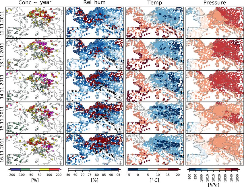
6396        G. Gašparac et al.: Regional modelling for the assessment of PM10 at rural background locations in Europe

ameter ≤ 2.5 µm (PM2.5 ) and ≤ 10 µm (PM10 ) for continen-         ilar underestimations of PM concentrations. Applications of
tal Europe are strongly affected by regional aerosol transport.    the Weather Research and Forecasting model with Chem-
For example, long-range transport has been attributed to con-      istry, the WRF-Chem model (Grell et al., 2005), showed a
tributing up to about three-quarters of the total urban PM2.5      relatively good comparison with measurements of the total
concentrations in Finland (Karppinen et al., 2004; Pakkanen        PM mass over Europe (Tuccella et al., 2012), but the model
et al., 2001). A large fraction of the urban population is ex-     did not capture the trends of PM compounds. Other studies
posed to levels of PM10 in excess of the limit values set          (e.g. Saide et al., 2011) also indicated challenges in the mod-
for the protection of human health by national and interna-        elling of PM mass, especially during statically stable atmo-
tional bodies. There have been numerous recent policy initia-      spheric conditions, due to the choice of vertical and horizon-
tives that aim to control PM concentrations to protect human       tal resolution as well as the influence of vertical and horizon-
health (EEA, 2015); yet high levels are reported regularly         tal diffusion coefficients during model set-up (Jeričević et al.,
in different parts of the world (Kumar et al., 2015, 2016).        2010). Furthermore, the WRF-Chem model was extensively
The main problem in the assessment of PM10 is in its di-           tested during the intensive evaluation of online coupled mod-
verse chemical composition across Europe. Nitrate is a main        els of the second phase of the Air Quality Model Evalua-
contributor in northwest (NW) Europe, mineral dust in south        tion International Initiative (AQMEII, 2012). During the ex-
(S) Europe, desert dust from Africa over the Mediterranean,        ercise, overall underestimation of PM concentrations for all
carbon in central Europe and sea salt in coastal areas of Eu-      the stations was found, due to a relatively coarse grid spac-
rope. The total residence time of PM in the atmosphere is          ing (23 km) together with the overestimation of wind speed,
highly dependent on precipitation, which influences the de-        which can result in fast removal of pollutants from urban
position processes. Conversely, wind speed plays an impor-         sources and underprediction of secondary organic aerosol
tant role in both PM advection and the alteration of PM size       (SOA) and grid-scale precipitation (e.g. Baró et al., 2015;
and composition. PM10 usually deposits at closer distances         Forkel et al., 2015). The EMEP performance is evaluated
from its sources than smaller particles (e.g. Dimitriou and        through continuous yearly technical reports such as EMEP
Kassomenos, 2014). On average, the residence time of fine          (2016). The most recent studies showed significant technical
particles (PM2.5 ) is usually about 4–6 d as opposed to 1–2 d      improvements with updated initial and boundary conditions
for coarser particles (PM2.5−10 ). The typical distances for de-   as well as with newer model versions, which include various
position from the sources are around 2000 to 3000 km for the       modifications in the chemistry modules. Throughout the per-
fine particles and 500 to 1000 km for coarse particles (WHO,       formed extensive tests (Gauss et al., 2016), the model gen-
2006). PM10 can be emitted directly to the atmosphere from         erally underestimated the observed annual mean PM10 lev-
various natural and anthropogenic sources (primary PM10 )          els by 24 %. However, there was an overall relatively good
or can be produced through photochemical reactions in the          agreement (correlation coefficient, r = 0.74) between mod-
atmosphere (secondary PM10 ). In addition, wind-blown soil         elled and measured annual mean PM10 concentrations. A
and resuspended street dust contribute largely to the coarse-      number of AQMs are currently available for practical appli-
particle fraction (Amato et al., 2009; Forsberg et al., 2005;      cations. These models can be broadly divided into two main
Harrison and Jones, 2005; Jeričević et al., 2012; Kumar and      groups: offline and online models. The offline models con-
Goel, 2016; Luhana et al., 2004; Putaud et al., 2004). The         sider solving separately meteorological conditions prior to
contribution to PM emissions can be relevant at spatial scales     chemistry during the simulation runs. There exists a huge
ranging from local to regional including long-range transport      variety of offline models such as the Comprehensive Air
(e.g. Juda-Rezler et al., 2011; Querol et al., 2004).              Quality Model with Extensions, CAMx (EVIRON, 2010);
   Air quality models (AQMs) play a significant role in the        the Community Multi-scale Air Quality, CMAQ (U.S. Envi-
assessment and management of air quality. These are widely         ronmental Protection Agency); EMEP; and LOTOS-EUROS
used in public health cohort studies given that the measure-       (e.g. Solazzo et al., 2012). In contrast to offline models, the
ments are expensive and usually represent limited and small        online models were developed to include the more consis-
areas, e.g. rural areas or mountains (Ritter, 2013). Previ-        tent description of processes such as atmospheric turbulence
ous research on PM mass modelling (e.g. Vautard et al.,            and to use a more frequent update of the meteorological
2007) identified the general underestimation of PM mass            variables within the chemistry part of the model. There are
from large-scale models (grid spacing ∼ 50 km) and the diffi-      other reasons for online coupling such as the ability to treat
culties in capturing the observed seasonal variations in an ur-    feedback processes between aerosols and airflows. Exam-
ban location. The complexity of PM mass modelling was also         ples of online models include WRF-Chem, the Environment
introduced in Prank et al. (2016) where various modelling          – High-Resolution Limited Area Model (Enviro-HIRLAM),
systems were compared – the Unified European Monitor-              the Consortium for Small-scale Modelling Aerosols and Re-
ing and Evaluation Programme, EMEP (e.g. Simpson et al.,           active Trace gases (COSMO-ART), and the non-hydrostatic
2012), LOTOS (e.g. Schaap et al., 2008), SILAM (e.g. Sofiev        mesoscale atmospheric model with climate module (Meso-
et al., 2008), and CMAQ (Community Multi-Scale Air Qual-           NH-C); see, e.g., Baklanov et al. (2014).
ity; Environmental Protection Agency) – which showed sim-

Atmos. Chem. Phys., 20, 6395–6415, 2020                                              https://doi.org/10.5194/acp-20-6395-2020
G. Gašparac et al.: Regional modelling for the assessment of PM10 at rural background locations in Europe                   6397

   The main objective of this research was to investigate         Agency       (https://www.eea.europa.eu/data-and-maps/data/
the spatial and temporal variability in background PM             airbase-the-european-air-quality-database-7, last access:
concentrations using 1 year of observed data, to evaluate the     12 May 2020), and the database developed under the
regional AQM performance in simulating PM concentrations          EU-funded PHARE 2006 project Establishment of Air
during the colder part of the year and to analyse and evaluate    Quality Monitoring and Management System, where 12
the episodes of regionally increased PM concentrations that       new rural stations were established in Croatia for PM
occurred in November 2011 in eastern and central Europe           measurements in 2011. For this study, PM10 concentrations
(the Pannonian Basin) during statically stable atmospheric        were available from six rural background stations in Croatia.
conditions followed by drought periods. In this particular        The monitoring stations were divided into three categories
case, the pollution problems appeared to be of consid-            based on their elevation to examine the spatial variability
erable concern in Hungary; e.g. smog alerts were issued           of pollution and to test the model performance at different
in Budapest and eastern Hungary, various cars with high           levels: (i) sea-level (altitude from 0 to 200 m), (ii) elevated
environmental impact were banned from the roads, and a ban        (from 200 to 500 m) and (iii) mountain stations (> 500 m).
was also issued on procedures such as burning leaves and          The differentiation of stations with respect to their elevation
garden debris (https://thecontrarianhungarian.wordpress.          is important when dealing with station representativeness
com/2011/11/08/hungarian-news-digest-nov-7-2011/, last            in models. According to current knowledge, it is found that
access: 12 May 2020). Based on the analysis in Spinoni            numerical models perform differently at higher altitudes.
et al. (2015), the Pannonian Basin was characterised as an        This is mostly related to the vertical resolution of the model
area with increased drought frequency per decade during           within the boundary layer (Bernier and Bélair, 2012). With
the period from 1950 to 2012. This can have a strong effect       respect to the elevation, the total numbers of stations used for
on air quality problems, e.g. a dust-bowl effect (Stahl et al.,   further analysis (Sect. 3.1) and model validation (Sect. 3.3)
2016). Further assessment is conducted by applying two            are shown in Table 1. When interpreting average observed
regional models: the offline Unified EMEP and the online          yearly, seasonal and episode PM10 concentrations, it is
coupled WRF-Chem in the simulation of PM mass transport.          important to note that the majority of the surface stations
Model results are compared against observed concentrations        are in northern and western Europe, while the elevated
at rural background sea-level, elevated and mountain stations     and mountain stations are generally situated in central and
in Europe.                                                        eastern Europe. The density of rural background stations
   Throughout the analysis, the indication of problems is         varies geographically with a significantly greater number
given in the application of both regional models in simulating    of stations in western and northern Europe compared
PM concentrations at different elevations (sea-level, elevated    to central and eastern Europe. The PM10 measurements
and mountain stations). We provide an individual validation       were acquired with different approaches: the gravimetric
of widely used different set-ups of the modelling systems         method (EN12341) using high-volume samplers (HVSs)
without harmonisation of emission and meteorological input        and low-volume samplers (LVSs), β-attenuation monitoring
fields. This is a different approach than in, e.g., AQMEII ex-    (e.g. Willeke and Baron, 1993), TEOMs (tapered element
ercises and enables an essential scientific baseline for choos-   oscillating microbalances) measurements (e.g. Patashnick
ing the appropriate model for future needs in terms of res-       and Rupprecht, 1980), and the optical particle counters
olution, physical parameterisation, emission dataset and the      of the GRIMM 180 instrument. The comparison of the
complexity of orography representation in practical applica-      PM10 concentration data obtained by different measurement
tions. Due to the complexity of air quality problems regard-      methods is still considered to be a complicated issue. The
ing PM, this work aims at filling the gaps in knowledge of        standard gravimetric method (EN12341) is a classic method
regional modelling of PM over eastern Europe in terms of          of weighing the mass deposited on a filter. It is accepted
less information about PM concentrations (EEA, 2013) and          as a standard reference method against which all other
therefore low accuracy in the PM emission inventory, and it       measurement methods are validated (Noble et al., 2001;
fits in with the problems addressed in most of the air quality    EC, 2010). Although this is a standard method used for
plans in Europe (Miranda et al., 2015).                           compliance reasons in the EU, there are numerous studies
                                                                  showing that chemical reactions between the air and the
                                                                  deposited particles, as well as within the aerosol mass, also
2     Methodology                                                 compromise these measurements. The ambient temperature
                                                                  and relative humidity greatly influence the actual mass
2.1    Measurements                                               loaded on the filter (Allen et al., 1997; Eisner and Wiener,
                                                                  2002; Pang et al., 2002). For example, aerosol particles
The measurements of PM10 from the rural background                can contain up to 30 % water at 50 % relative humidity
stations were taken from two available air quality                (Putaud et al., 2004). Conversely, calibration, temperature
databases. These were AirBase, the European air qual-             and humidity issues can create artefacts that must be taken
ity database maintained by the European Environmental             into account for TEOMs and β-attenuation monitoring

https://doi.org/10.5194/acp-20-6395-2020                                           Atmos. Chem. Phys., 20, 6395–6415, 2020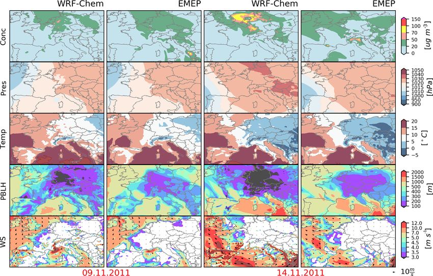
6398         G. Gašparac et al.: Regional modelling for the assessment of PM10 at rural background locations in Europe

Table 1. The number of stations used in the analysis.                a suite of different performance measures needs to be ap-
                                                                     plied. Results should be carefully interpreted by taking into
              Station         AirBase       Meteorology              account advantages and disadvantages of all applied statisti-
              altitude        stations          stations             cal measures and ensuring that those are complementary to
              Sea level           132               366              each other and lead to the same conclusion on the certain
              Elevated             85               335              ability of the model performance. Therefore as already pre-
              Mountain             93               219              viously noted in this section, a set of different statistical mea-
                                                                     sures is used in order to understand the ability of the model
                                                                     to properly estimate high-pollution episodes of PM10 con-
(Allen et al., 1997; Hauck et al., 2004). Lacey and Faulkner         centrations and to evaluate the relations between chemical
(2015) addressed three objectives for the treatment of               and meteorological parameters. BIAS refers to the arithmetic
uncertainties gained with PM measurements: estimate the              difference between M and O indicating the model’s general
uncertainty, identify the measurement with the greatest              overestimation or underestimation of analysed parameters. It
impact on uncertainty and finally determine the sensitivity of       is known that a model whose predictions are completely out
total uncertainty to all measured parameters. As is common           of phase with observations can still have a BIAS= 0 because
in these types of studies, the authors did not consider the          of compensating errors. Different BIAS was used: for eval-
uncertainty of measurements in further analysis.                     uating model performance regarding PM10 we used BIAS
                                                                     under Eq. (1) as opposed to meteorological parameters under
2.2    Statistical analysis                                          Eq. (2). r and IOA are dimensionless measures of model ac-
                                                                     curacy. r is sensitive to good agreement of extreme data pairs,
The evaluation of model performance is a comprehensive               and a scatter plot might show generally poor agreement, but
task. In order to evaluate and validate modelling perfor-            the presence of good agreement for a few extreme pairs will
mance, various statistical measures such as bias (BIAS),             greatly improve r. The IOA is the ratio of the mean square
index of agreement (IOA), correlation coefficient (r), root          error and the potential error and then subtracted from 1 (Will-
mean square error (RMSE), normalised mean square er-                 mott, 1984). The IOA varies from 0 to 1, with higher index
ror (NMSE), and systematic (NMSEsys ) and unsystem-                  values indicating that M have better agreement with the O.
atic (NMSEunsys ) normalised mean square error were used             Although the IOA provides some improvement over r, it is
(Chang and Hanna, 2004):                                             still sensitive to extreme values due to the square differences
                  !                                                  in the mean square error in the numerator. RMSE gives in-
          M −O                                                       formation on the spread of the residuals from the regression
BIAS =              × 100 %,                            (1)
             O                                                       line; it depends greatly on the magnitude of the parameter on
                                                                     which RMSE is applied and therefore it cannot be compared
BIAS = M − O,                                                  (2)
                             PN                                      with RMSE of some other parameter. NMSEsys is a measure
                              i=1 (Oi   − Mi   )2                    with which NMSEunsys provides information on systematic
IOA = 1 − PN                                               ,   (3)
                      − O) + abs(Oi − O))2                           and unsystematic (random) errors in the model.
               i=1 (abs(Mi
            P         P P
          n Oi Mi − Oi Mi                                            2.3   Boundary layer height determination
r=q P                q                  ,                      (4)
    n Oi2 − ( Oi )2 n Mi2 − ( Mi )2
               P          P      P
       v                                                             One of the widely used methods for deriving boundary layer
       u N
       u1 X                                                          height from numerical models is based on the assumption
RMSE = t       (Mi − Oi )2 ,                                   (5)   that turbulence collapses to laminar flow when the bulk
         n i=1                                                       Richardson number RiB , exceeds values of a critical RiB (∼
           (O − M)2                                                  0.25 and larger), and the height at which this occurs can be
NMSE =                   ,                                     (6)   considered as a boundary layer height (Jeričević et al., 2010).
              OM                                                     Using sounding and modelled data, RiB was calculated based
                         2
               4
                     O−M
                                                                    on the following expression and shown in Sect. 3.3.3:
                   O.5 O+M
NMSEsys =                     2
                                        ,                      (7)           g(z − z0 )     θ (z) − θ (z0 )
                                                                     RiB =                                  ,                       (9)

                         O−M
              4−                                                              θ (z)      (u(z))2 + (v(z))2
                       O.5 O+M

NMSE = NMSEsys + NMSEunsys ,                                   (8)   where z is the height of the particular model level, z0 is the
                                                                     height of the first level in the model, θ (z) is the potential tem-
where M stands for model predictions and O for observa-              perature at the height z, θ (z0 ) is the potential temperature at
tions.                                                               the height z0 , and θ (z) is the averaged potential temperature
   As there is no single best modelling performance mea-             between the first level (z0 ) and particular level (z). u(z) and
sure, it is recommended by Chang and Hanna (2004) that               v(z) are the wind components on particular levels.

Atmos. Chem. Phys., 20, 6395–6415, 2020                                                   https://doi.org/10.5194/acp-20-6395-2020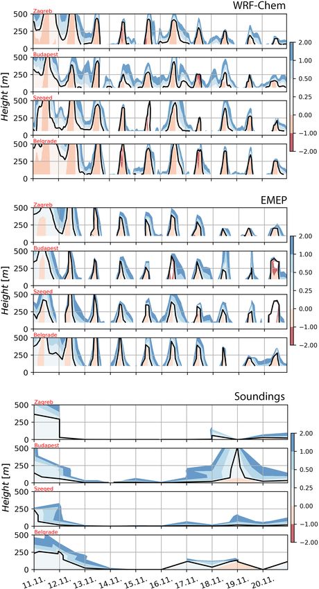
G. Gašparac et al.: Regional modelling for the assessment of PM10 at rural background locations in Europe                    6399

  Comparison of estimated planetary boundary layer height        bon monoxide (CO) and particulates (PM2.5 , and PM2.5−10 ).
(PBLH) was carried out using Eq. (9) rather than compar-         The PM categories can be further divided into elemental car-
ing the direct output of model-derived PBLH values as each       bon, organic matter and other compounds as required. Emis-
model uses a different method for the calculation of the         sions can be set from anthropogenic sources such as the
PBLH. By using the same methodology for PBLH determi-            burning of fossil and biomass-based fuels and solvent re-
nation, uncertainties are reduced and the more realistic eval-   lease or from natural sources such as foliar volatile organic
uation of two modelled PBLH values is ensured.                   compound (VOC) emissions or volcanoes. Several sources
                                                                 are challenging to categorise into anthropogenic versus natu-
2.4     Air quality models                                       ral categories (Winiwarter and Simpson, 1999), for example,
                                                                 emissions of NO from microbes in soils being promoted by
This work is based on the intensive tests performed in Gaš-      N-deposition and fertiliser usage. The anthropogenic emis-
parac et al. (2016), where the WRF-Chem, Unified EMEP            sions are categorised into 11 SNAP (Selected Nomenclature
and WRF-CAMx models were evaluated against the sur-              for sources of Air Pollution) sectors based on their sources.
face measurement stations over Croatia under different at-       Emission integration during simulation is distributed verti-
mospheric static stability conditions. Here, both EMEP and       cally, based on the SNAP sectors and plume-rise calculations
WRF-Chem AQMs are used to determine the spatial and              performed for different types of emission sources and, tem-
temporal distribution of PM10 concentrations and possible        porally, based upon time factors (i.e. monthly, daily, day of
transboundary transport and to evaluate the performance of       week, weekly, hourly).
the individual model systems during a 1-month period at the         Regarding the planetary boundary layer parameterisations
sea-level, elevated and mountain rural background stations       under statically stable atmospheric conditions, EMEP in-
in Europe. The WRF-Chem simulation is performed from             cludes a non-local vertical diffusion scheme based on a lin-
29 October to 30 November and EMEP from 1 October to             ear exponential profile with coefficients calculated from large
30 November. As all statistical analysis was done for dates      eddy simulation (LES) data and boundary layer height de-
after 1 November the simulation length was long enough to        termined using the bulk Richardson number method (Jeriče-
overcome the effects of spin-up time.                            vić and Večenaj, 2009; Jeričević et al., 2010; Simpson et al.,
                                                                 2012). Other mechanism used in this work (e.g. chemical
2.4.1    The EMEP model                                          scheme: EmChem09; chemical preprocessor: GenChem) are
                                                                 described in Simpson et al. (2012).
The EMEP chemical transport model (Simpson et al., 2012),           The above set-up of the EMEP model with the IFS mete-
developed by the Meteorological Synthesizing Centre-West         orology as an initial and boundary meteorological condition
(MSC-W) was used to perform calculations of PM10 concen-         is later on referred to and used as the “EMEP model”. Any
trations (http://www.emep.int/, last access: 12 May 2020).       further comparison of meteorological conditions obtained in
The model domain encompassed all of Europe with a hori-          EMEP simulations is related to the IFS model and PM10 to
zontal grid spacing of 50×50 km2 , extending vertically from     the choice of EMEP chemistry parameterisation.
surface level (first model level height around 42 m) to the
tropopause at 100 hPa, as seen in the Supplement Fig. S1.        2.4.2   The WRF-Chem model
The basic physical formulation of the EMEP model is de-
rived from Berge and Jakobsen (1998). The model derives          The WRF-Chem model is the WRF (Weather Research and
its horizontal and vertical grid from the input meteorolog-      Forecasting) model (http://www.wrf-model.org, last access:
ical data. The daily meteorological input data used for the      12 May 2020) coupled with chemistry. It is a state-of-the-art
EMEP/MSC-W model for 2011 were based on experimen-               air quality model (Grell et al., 2005), in which the chem-
tal forecast runs with the Integrated Forecast System (IFS),     istry (emission, transport, mixing, and chemical transforma-
a global operational forecasting model from the European         tion of trace gases and aerosols) is simultaneously simu-
Centre for Medium-Range Weather Forecasts (ECMWF).               lated with meteorology (online coupling). The WRF is a
Vertically, the 60 eta levels of the IFS model were interpo-     mesoscale numerical weather prediction system designed
lated onto the 37 EMEP sigma levels. The emission input for      for operational forecasting needs and atmospheric research
the EMEP/MSC-W model, with a horizontal grid spacing of          (Skamarock et al., 2008). The model set-up was based on ear-
50 × 50 km2 , consists of gridded annual national emissions      lier research (Gašparac et al., 2016; Grgurić et al., 2013; Jer-
based on emission data reported every year to EMEP/MSC-          ičević et al., 2017) where the results were evaluated against
W (until 2005) and to the Centre on Emission Inventories and     measurements at meteorological stations in Croatia. In this
Projections (from 2006) by each participating country. The       paper, we used the WRF-Chem version 3.5.1. A Mercator
standard emissions input required by the EMEP model con-         projection was used in a one-domain run on 170 points in the
sists of gridded annual national emissions of sulfur dioxide     east–west direction and 145 points in the north–south direc-
(SO2 ), nitrogen oxides (NOx =NO + NO2 ), ammonia (NH3 ),        tion, with a cell size of 18 × 18 km2 (Fig. S1) and a verti-
non-methane volatile organic compounds (NMVOCs), car-            cal grid spacing encompassing the atmosphere from surface

https://doi.org/10.5194/acp-20-6395-2020                                          Atmos. Chem. Phys., 20, 6395–6415, 2020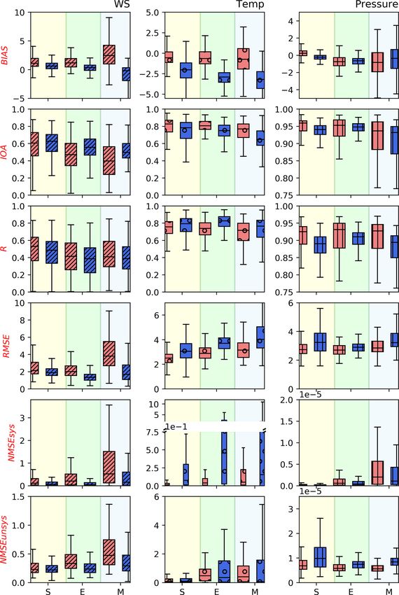
6400            G. Gašparac et al.: Regional modelling for the assessment of PM10 at rural background locations in Europe

level (first model level height around 22 m) to the height of
∼ 23 km in 50 unequally sorted sigma levels that were more
densely distributed near the ground level. Initial and bound-
ary meteorological conditions were provided by NCEP (Na-
tional Centers for Environmental Prediction) Final Analysis
(FNL ds083.2) with 1◦ of horizontal resolution and a time
step of 6 h. They were selected based on previous research
and other conducted studies with the WRF or WRF-Chem
model (Gašparac et al., 2016; Grgurić et al., 2013; Jeričević
et al., 2017; Syrakov et al., 2015). FNL analyses are a product
of the Global Data Assimilation System (GDAS), which con-
tinuously makes multiple analyses of collected observational
data from the Global Telecommunications System (GTS) and
various other sources. The whole analysis is available at 26
pressure levels from the surface to a height of ∼ 28 km. The
input emissions were prepared via the PREP-CHEM Sources
tool (Freitas et al., 2011) with the EDGAR (version 4.3.1.,
Emissions Database for Global Atmospheric Research) in-             Figure 1. Number of days exceeding the daily limit PM10 value
ventory for the year 2011. Biogenic emissions were cal-             (LV) at rural background stations during the year 2011 in the do-
culated from MEGAN (Model of Emissions of Gases and                 main of the research. Stations marked with a grey circle repre-
Aerosols from Nature; Guenther et al., 2006) and lateral            sent less than or equal to 35 permitted exceedances during the year
                                                                    (2008/50/EC Directive).
boundary and initial conditions were created from the global
chemistry model MOZART (Emmons et al., 2010). The de-
tailed WRF-Chem set-up is shown in Table 2.
   It is worth pointing out that the results of statistical anal-   stations showed that observed (PM10 )d exceeded LV 5456
ysis and model evaluation further on in the text will not de-       times during 2011 and were mainly located in the hotspot
scribe the performance of the model itself but rather will de-      areas (Fig. 1). The seasonal variation in (PM10 )d during
scribe the performance of a set of selected parameterisations       2011 was significant at the 5 % level (based on analysis of
and chemical and meteorological initial and boundary condi-         variance, ANOVA; p = 0). The applied ANOVA is calcu-
tions used in the WRF-Chem model. Following this, when re-          lated via scipy python package. This particular one-way
ferring to the “WRF-Chem model” in the text, the authors are        ANOVA tests the null hypothesis that two or more groups
referring to the WRF-Chem model with the above-described            have the same population mean. The p value is common vari-
set-up (Table 2).                                                   able used in hypothesis testing, the smaller the p value, the
                                                                    stronger is the evidence that the hypothesis needs to be re-
                                                                    jected (Heiman, 2001).
3     Results                                                          Spatially averaged seasonal values of (PM10 )d were 21.62,
                                                                    21.74, 14.96 and 20.87 µg m−3 for DJF, MAM, JJA and
Available daily averaged rural background PM10 concentra-           SON, respectively. Only during summer (JJA) was a de-
tions ((PM10 )d ) over Europe (Table 1) were analysed in the        crease found with respect to other seasons over Europe. How-
following sections with annual temporal variations and the          ever, it should be noted that significant differences in PM
episodes of very high (PM10 )d concentrations that occurred         levels across Europe are recognised (Putaud et al., 2004)
during November 2011.                                               and a deeper analysis of spatial and temporal variations in
                                                                    background PM10 concentration is needed. Fig. 2 presents
3.1    Analysis of PM measurements                                  individual (PM10 )d values for each rural background sta-
                                                                    tion (panel b), spatially averaged (PM10 )d over the all sta-
We analysed the (PM10 )d measurements from 310 stations             tions (green line, panel a) and the maximum (PM10 )d val-
over a period of 1 year during 2011. Following the air              ues among all rural background stations (red line, panel a)
quality report in Europe (EEA, 2013), (PM10 )d limit val-           during 2011. The time series of these (PM10 )d concentra-
ues (2008/50/EC Directive, LV = 50 µg m−3 ) were exceeded           tions indicate the increase in concentrations at all rural back-
at both urban and rural sites in Europe during 2011. These          ground stations (Fig. 2) during DJF and SON seasons (i.e.
“hotspots”, locations with exceedances of the LV, were in           the colder part of the year). During these seasons, (PM10 )d
south Poland, the Czech Republic, the Po Valley, the Balkan         values at all rural background stations were relatively high,
Peninsula, Portugal and Turkey. In this work, we focused            reaching 40 µg m−3 . During the colder part of the year, most
on the area and rural background stations shown in Fig. 1.          of the stations recorded (PM10 )d values above the permitted
The analysis of measurements from 310 rural background              LV which is mainly due to increased emissions from domes-

Atmos. Chem. Phys., 20, 6395–6415, 2020                                               https://doi.org/10.5194/acp-20-6395-2020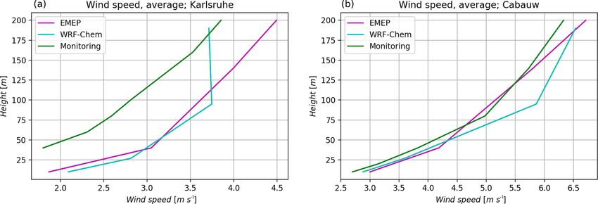
G. Gašparac et al.: Regional modelling for the assessment of PM10 at rural background locations in Europe                         6401

Table 2. Details of the WRF-Chem parameterisations.

                      Parameterisation                    Scheme used
                      Microphysics                        Lin et al. scheme
                      Long-wave radiation                 Rapid radiative transfer model (rrtm) scheme
                      Short-wave radiation                Goddard short wave
                      Land surface model                  Unified Noah land surface model
                      Surface layer                       Monin–Obukhov (Janjić) scheme
                      Boundary layer scheme               Mellor–Yamada–Janjić turbulent kinetic energy (TKE) scheme
                      Cumulus physics                     Kain–Fritsch (new Eta) scheme
                      Gas-phase mechanism                 RADM2
                      Aerosol module                      MADE/SORGAM (including some aqueous reactions)
                      Chemical initial conditions         From MOZART global model
                      Chemical boundary conditions        Idealised profile (from MOZART global model)

                                                                          sphere over Europe. According to Blunden et al. (2012), a
                                                                          strong high-pressure field encompasses the area over cen-
                                                                          tral and southern Europe during November 2011. Moreover,
                                                                          this month was the coldest in 2011 and extremely dry; it
                                                                          was the driest month in Bulgaria and Serbia with less than
                                                                          25 % of the national total averaged precipitation. During the
                                                                          SON season in 2011, anticyclonic conditions prevailed and
                                                                          below-average precipitation conditions were recorded. Fol-
                                                                          lowing Cindrić et al. (2016), the drought was present in
                                                                          the continental part of Croatia, encompassing the Pannonian
                                                                          Basin and surrounding countries, and was characterised by
                                                                          an extremely long duration. It started in February 2011 and
Figure 2. The spatial average (a) over all the rural background sta-
tions (the green line, corresponding to the right green y axis) and the
                                                                          reached the most intense extremely dry conditions in Novem-
maximum of (PM10 )d for all rural background stations (the red line,      ber, when an increase in (PM10 )d was recorded at the ma-
corresponding to the left red y axis) and (PM10 )d (b) during 2011.       jority of the analysed rural background stations (Fig. 2). In
The values above 50 µg m−3 (red colour) represent values above the        western Europe, the autumn season temperature was above
daily limit values for PM10 under the 2008/50/EC Directive.               average normal (1961–1990) and was characterised by a pre-
                                                                          vailing high-pressure field. This was observed particularly
                                                                          in November, during which monthly average temperature
tic heating and industrial activities (EEA, 2013). Moreover,              records were exceeded (e.g. UK, France and Switzerland re-
according to, e.g., EEA (2013) and Saarikoski et al. (2008),              ported their second warmest autumn in last 100 years). Con-
aside from the primary sources (natural and anthropogenic),               trary to the western Europe, the increased nocturnal cooling
the secondary inorganic aerosols (SIAs) and SOAs vary sub-                decreased temperatures in southeastern Europe. The domi-
stantially across Europe from season to season, which indi-               nating high-pressure field resulted in a decrease in precip-
cates the presence of various PM10 sources. SIA contribu-                 itation in some western and central Europe countries, e.g.
tions are mostly related to SON–DJF, domestic heating and                 southern France, the Alpine region, Germany, Austria, the
large combustion plants, while SOA contribution is instead                Czech Republic, Slovakia and Hungary. All those countries
related to MAM–JJA seasons, e.g. emissions from vegeta-                   reported the driest November in more than the last 100 years
tion. This can explain the relatively high daily concentrations           (Blunden et al., 2012). In order to identify the episodes and
in the MAM season (Fig. 2).                                               the areas of enhanced (PM10 )d values, differences (DFs) be-
                                                                          tween the (PM10 )d and annually averaged PM10 ((PM10 )a )
3.2   Analysis of PM measurements and meteorological                      at rural background stations were used, defined as
      conditions during episodes in November 2011                                (PM10 )d − (PM10 )a
                                                                          DF =                       × 100 %.                      (10)
Further analysis of the observed and modelled (PM10 )d val-                          (PM10 )a
ues is focused on November 2011, as the highest (PM10 )d                  The spatial distribution of DF values in percentage is shown
concentrations were present during the colder part of the year            in Fig. S2. The significant increase in (PM10 )d is defined as
and prevailing meteorological conditions enabled the accu-                an increase in DF of more than 100 % with respect to the
mulation of the pollutants in the lower layers of the atmo-               annual mean. If a significant increase in DF was detected

https://doi.org/10.5194/acp-20-6395-2020                                                   Atmos. Chem. Phys., 20, 6395–6415, 2020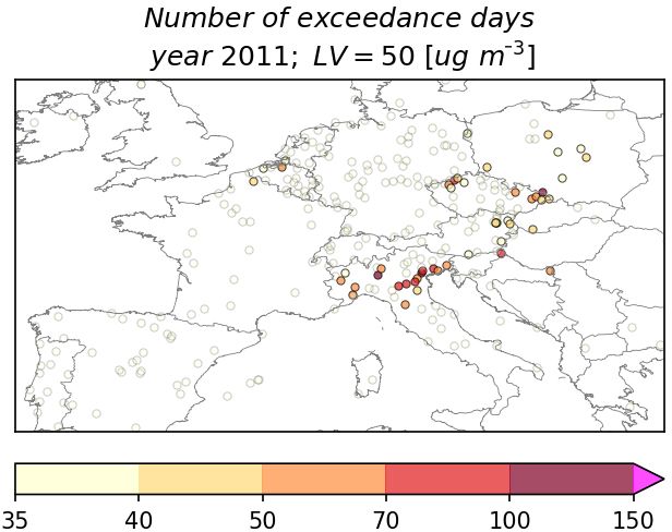
6402        G. Gašparac et al.: Regional modelling for the assessment of PM10 at rural background locations in Europe

and lasted at least 2 consequent days, the area was identi-        3 m s−1 over all of Europe (not shown); values were reduced
fied as an area experiencing a high-pollution episode. Dur-        and comparable to (PM10 )a (Fig. S2).
ing November 2011, a significant increase in (PM10 )d oc-             A building up of (PM10 )d started again from 12 Novem-
curred generally over the addressed hotspots within the do-        ber (Figs. S2 and 4), mainly affecting stations in central
main, and two high-pollution episodes (DF > 100 %) were            and coastal western Europe. The observed concentrations
found (Figs. 3–4). During both episodes identified, the high-      exceeded the annual averages by up to 100 % (DF) affect-
est peaks (9 November in the first episode, Fig. 3; 14 Novem-      ing the areas with hotspots (southern Poland, the Czech Re-
ber in the second episode, Fig. 4) occurred in the area of         public, Benelux countries) and up to 200 % in central Ger-
central Europe and coastal part of western Europe with a           many and Slovakia (Fig. 4). In the following days, from 13
DF above 200 %. Later on, observed meteorological condi-           to 16 November, increased concentrations (DF > 100 %) en-
tions (daily averaged sea-level pressure field ((mslp)d ), daily   compassing the area from central Europe in the northwest di-
averaged surface temperature ((t2 m )d ), daily averaged rela-     rection through coastal areas in Germany, the UK and Ireland
tive humidity ((rh)d ), Figs. 3–4; daily averaged surface wind     were present in the southeastern direction across the Czech
speed ((ws)d ) and direction ((wd)d ), Fig. 5) along with the      Republic, Austria, Slovenia, western Hungary and Croatia.
DF (Figs. 3–4) were analysed to determine the mechanisms           During this, second episode, a high-(mslp)d field again influ-
and relationships between the meteorology and the high-            enced the weather conditions (Fig. 4). Low (ws)d ( 200 %,
Po Valley, Balkan Peninsula; Fig. S2). On 3 November, cy-          Poland, Germany, Slovakia, the Czech Republic; Fig. 4), an
clone Rolf in the Gulf of Genoa generated intense rainfall in      increase in (rh)d was found, except in the Pannonian Basin
northern Italy (not shown). These conditions were followed         (Fig. S3) where relatively lower (rh)d and higher (t2 m )d val-
by high S to SE winds over the Adriatic Sea and nearby             ues of up to 20 % and 5 ◦ C, respectively, were recorded in
countries in the following days (Blunden et al., 2012). The        comparison with the surrounding areas. Moreover, within the
characteristic meteorological conditions during or following       areas of the Pannonian Basin, a high (mslp)d and low wind
Genoa low cyclones are a strong flow aloft (Sirocco wind           speed conditions prevailed for 1 d longer (Figs. 4–5, right) in
over the Adriatic Sea and Italy), rainfall in mid-central Eu-      comparison with the surrounding areas. On 19 November a
rope (Austria, the Czech Republic and Poland) and the for-         large-scale decrease in (PM10 )d was detected and values of
mation of high-(mslp)d fields over eastern Europe (Blunden         (PM10 )d were generally reduced to those of (PM10 )a at all
et al., 2012). From 5 November, a first large-scale episode        stations (Figs. S2, S6).
(DF > 100 %, Fig. S2) started in central and northern Eu-
rope. The onset of the event was in Poland and northeastern        3.3   Model evaluation
Germany and encompassed the coastal areas of northern Eu-
rope, the Benelux countries and northern France in the fol-        Numerical simulations using the EMEP (with a grid spac-
lowing days until 9 November. During the first episode, a          ing of 50 × 50 km2 ) and WRF-Chem (with a grid spacing of
high-(mslp)d field (Fig. 3) formed over continental Europe,        18 × 18 km2 ; Fig. S1) models were provided for November
first affecting the east of Europe and gradually spreading to      2011 to evaluate the performances of the individual, state-of-
western Europe. Over the affected area (DF > 100 %, Fig. 3),       the-art models during November 2011 and to further inves-
the wind speed was generally reduced below 3 m s−1 , except        tigate the processes contributing to the increased concentra-
at some isolated stations (Fig. 5, left). Moderate to strong       tions during the high-pollution episodes. It is worth noting
NE wind (5–6 m s−1 ) started to blow in coastal and northern       that differences between the emission databases used were
Europe from 7 November until the end of the first episode,         found in the spatial variability of PM10 emissions and in
when they turned into an ESE direction (Fig. 5, left). Over        the gridded input emission fields above the entire domains
the mountainous region in central Europe (the Czech Re-            of EMEP and WRF-Chem. Notable differences in emissions
public, Slovakia and south Germany), the wind speed was            were found over the coastal areas and eastern part of the do-
persistent during the episode, with relatively high magnitude      main, particularly over Bosnia and Herzegovina, Serbia and
(above 7 m s−1 ) and generally in a SSE direction. Over the        Hungary which are crucial for the case studies analysed here.
area with increased concentrations (DF > 100 %, Fig. 3), a         Aside from this, the difference in vertical resolution (first
gradual moderate decrease in (t2 m )d from east to west from       model level height – EMEP at 46 m, WRF-Chem at 22 m)
the beginning to the end of the first episode was found (i.e.      can have a strong impact on surface concentrations and thus
Poland < 0 ◦ C, Germany, the Czech Republic and Slovakia           can be related to the differences in surface PM10 concentra-
0–5 ◦ C). On 10 November the wind speed was lower than             tions obtained from the two models used.

Atmos. Chem. Phys., 20, 6395–6415, 2020                                             https://doi.org/10.5194/acp-20-6395-2020
G. Gašparac et al.: Regional modelling for the assessment of PM10 at rural background locations in Europe 6403
Figure 3. DF as “Conc ∼ year” and measurements from synoptic stations (relative humidity (Rel hum), ambient temperature at 2 m (Temp)
and surface pressure) from Ogimet (https://www.ogimet.com/, last access: 12 May 2020) during the first large-scale episode (5 to 9 Novem-
ber). Stations with a temperature between 0 and 5 ◦ C are marked with little grey dots due to better representativeness on the map.
3.3.1 Evaluation of model performances during level for EMEP. The relatively coarse horizontal resolutions
November 2011 of the models have a great impact on wind values (e.g. Jer-
ičević et al., 2012), which is why the modelled values cor-
Meteorological conditions respond better to the observed wind values at the Cabauw
site, situated in flat terrain, than to the values observed over
the moderately complex terrain at the Karlsruhe site. Above
Vertical wind profile plays an important role in the disper- 100 m, a change in the slope of the vertical wind speed pro-
sion of particulate matter. Hence, a validation of the mod- file for WRF-Chem was found. The difference in model per-
elled wind speed against measurements using mast-mounted formance above the surface layer was previously attributed
instruments (Fig. 6; Cabauw, Netherlands, 51.97◦ N, 4.95◦ E, to the proper choice of boundary layer parameterisation in
and Karlsruhe, in the western part of Germany, 48.98◦ N, Boadh et al. (2016).
8.39◦ E) was performed. During November there was no The modelled (ws)d , (t2 m )d and (mslp)d were com-
significant difference between modelled vertical profiles of pared to measurements from 920 synoptic stations within
wind speed below 75 m (Fig. 6) for both sites. Modelled ver- the domain taking into account the elevation of the sta-
tical wind profiles were close to measurements at the Cabauw tion. A detailed statistical evaluation of the two indi-
site (up to 75 m), while at Karlsruhe the models underes- vidual model performances was conducted by calculation
timated the observed wind speed values in the first 180 m and analyses of six different statistical measures (Fig. 7):
for the WRF-Chem model and much higher above ground
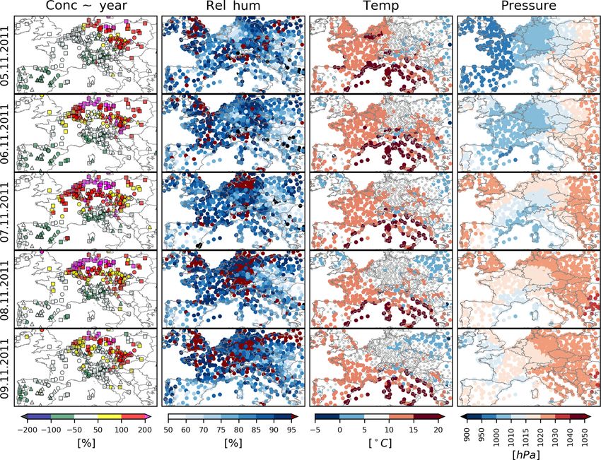
https://doi.org/10.5194/acp-20-6395-2020 Atmos. Chem. Phys., 20, 6395–6415, 20206404 G. Gašparac et al.: Regional modelling for the assessment of PM10 at rural background locations in Europe Figure 4. Same as Fig. 3, but during the second large-scale episode (12 to 16 November). BIAS((ws)d , (t2 m )d , (mslp)d ), IOA((ws)d , (t2 m )d , (mslp)d ), at mountain stations. WRF-Chem successfully predicted r((ws)d , (t2 m )d , (mslp)d ), RMSE((ws)d , (t2 m )d , (mslp)d ), (mslp)d and (t2 m )d as BIAS((mslp)d , (t2 m )d ) values were NMSEsys ((ws)d , (t2 m )d , (mslp)d ) and NMSEunsys ((ws)d , very low at sea level and elevated stations while small to (t2 m )d , and (mslp)d ). In the following Fig. 7, individual moderate (BIAS((mslp)d )∼ 1.2 hPa, BIAS((t2 m )d ) ± 1 ◦ C) scales for each analysed meteorological parameter are given at mountain stations. The BIAS ((mslp)d ) increases with as their magnitudes differs greatly. Statistic measures calcu- height for both models. On elevated stations, a median of lated for wind speed are given in units of metres per sec- BIAS((mslp)d ) decreased up to 1 hPa for both models. On ond, temperature in degrees Celsius and pressure in hec- mountain stations the spread of BIAS((mslp)d ) is higher topascal. This is important for the interpretation of model with respect to lower altitudes (−5 to 2.6 hPa for WRF- scores in simulating different meteorological parameters as, Chem and −4.9 to 4 hPa for the EMEP model). The me- e.g., RMSE or NMSE depend on their magnitude. Further- dian of BIAS((mslp)d ) is the same as for elevated sta- more, the results from Fig. 7 should be viewed as individ- tions for the WRF-Chem model and 0.5 hPa for the EMEP ual model performance rather than inter-comparison of two model. The EMEP model predicted (ws)d and (mslp)d well different model performances. According to BIAS((ws)d ), with low BIAS values at sea-level and elevated stations, the WRF-Chem model generally overestimated the observed while for surface (t2 m )d values, underestimation was found (ws)d , which is in accordance with other similar studies (BIAS((t2 m )d ) ∼ −2, 3 and 4 ◦ C at sea-level, elevated and (e.g. Solazzo et al., 2012). The median of overestimation of mountain stations, respectively). The median IOA((t2 m )d ) (ws)d increases with the station altitude; BIAS((ws)d ) was was relatively high for both models, while for IOA((ws)d ) it 1.8 m s−1 at sea-level, 1.9 m s−1 at elevated and 2.8 m s−1 was to a small extent lower. For both parameters a decrease Atmos. Chem. Phys., 20, 6395–6415, 2020 https://doi.org/10.5194/acp-20-6395-2020
G. Gašparac et al.: Regional modelling for the assessment of PM10 at rural background locations in Europe                          6405

Figure 5. Daily averaged wind speed and directions during two high-pollution episodes: from 5 to 9 November (episode 1, left) and from 12
to 16 November (episode 2, right). Stations with a measured wind speed below 3 m s−1 are marked with grey dots. Source of measurements:
Ogimet (https://www.ogimet.com/, last access: 12 May 2020).

in performance with height was found. This indicates prob-             stantial unsystematic and systematic errors for (mslp)d . The
lems in simulations with regional models over complex ter-             range of both systematic and unsystematic errors increased
rain, which is confirmed by the values of r that were consis-          with height for (t2 m )d ; the median values of NMSEsys and
tent for both models. As a result of small BIAS((mslp)d ) over         NMSEunsys ((t2 m )d ) for the EMEP model were the highest
sea-level and elevated stations, the IOA((mslp)d ) was close           for elevated stations. In the case of the WRF-Chem model,
to 1. However, over the mountain stations a high spread of             NMSEsys ((t2 m )d ) increases with height, while for the EMEP
values was found as the formulation of IOA is very sensitive           model, the highest NMSEunsys ((t2 m )d ) median was found at
to the extreme values. The models did not show any sub-                elevated stations.

https://doi.org/10.5194/acp-20-6395-2020                                                 Atmos. Chem. Phys., 20, 6395–6415, 2020
6406        G. Gašparac et al.: Regional modelling for the assessment of PM10 at rural background locations in Europe

Figure 6. Vertical profiles of measured and modelled wind speeds at Karlsruhe (a, measurement source: Institute of Meteorology and Climate
Research, Atmospheric Environmental Research, Karlsruhe Institute of Technology) and the Cabauw mast station (b, measurement source:
Cesar Observatory, http://www.cesar-observatory.nl, last access: 12 May 2020) during November 2011.

   Overall, during a 1-month period of simulation, EMEP had            tions. The average values over the domain for the WRF-
the lowest systematic errors for (ws)d , while WRF-Chem had            Chem and EMEP models were 0.39, 0.21 and 0.19 and 0.48,
the lowest systematic errors for (t2 m )d . Based on the statis-       0.28 and 0.24 for sea-level, elevated and mountain stations,
tics given, overall model performance regarding meteorolog-            respectively. High variability in r values over the domain for
ical parameters was in accordance with similar modelling               both models is found (Figs. S4–S5). As r is a measure of lin-
studies. For example, negative BIAS and high r for (t2 m )d            earity and is highly dependent on the estimation of peak val-
was found in, e.g., Skjøth et al. (2015) and Qu et al. (2014).         ues and trends, the low values at all stations are attributed to a
Positive BIAS for (ws)d was already addressed as an issue              mismatch between modelled and measured peak values dur-
in related studies such as, e.g., Baró et al. (2015) and Forkel        ing the period of analysis. Even a small discrepancy between
et al. (2015), while results for (mslp)d for sea-level and/or el-      measured and modelled (PM10 )d can lead to a decrease in r.
evated stations are in accordance with, e.g., Qu et al. (2014).        RMSE((PM10 )d ) decreases with height, and the highest me-
                                                                       dian RMSE values were found over sea-level stations (20.7
Chemistry                                                              for the WRF-Chem model and 17.3 for the EMEP model;
                                                                       Fig. 8, Table S1). It should be noted that RMSE depends
The modelled (PM10 )d values were compared with the avail-             greatly on the concentration magnitudes. Higher values of
able corresponding measurements (Table 1) with respect to              RMSE for both models generally correspond to the stations
height by applying statistical measures (Fig. 8, Table S1). Al-        with low r values (the hotspot areas: southern Poland, the
though the number of stations varies within altitude groups            Czech Republic, Po Valley; Figs. S4–S5). Figure 8 shows
(Table 1), the overall model performance can be inferred               that the trends of systematic errors differ between the mod-
from the above-mentioned figure and table. The underesti-              els. The lowest errors in the WRF-Chem model were found
mation of concentrations was found at sea-level (the median            over sea-level stations, while the highest were found over el-
of −44 % and −26 % for the WRF-Chem and EMEP models,                   evated stations. The errors in the EMEP model were com-
respectively) and elevated stations (−55 % and −29 % for               parable at all altitudes; however, the range of errors in-
the WRF-Chem and EMEP models, respectively; Figs. S4–                  creased with height. A similar performance was found for
S5). At mountain stations, EMEP had good agreement of                  the EMEP model and unsystematic errors. The median val-
∼ 13 %, while underestimation with respect to WRF-Chem                 ues were comparable at all altitudes, while the range slightly
is still present (∼ 33 %). According to Figs. S4–S5, the               increased with height. In the case of the WRF-Chem model, a
BIAS((PM10 )d ) in both model simulations showed a sim-                moderate increase in the median and the range of unsystem-
ilar distribution with respect to the height of the station,           atic errors with height was found. The areas affected with
i.e. moving from underestimation towards overestimation.               increased NMSEunsys ((PM10 )d ) were the hotspot areas (Po
IOA((PM10 )d ) was generally equally persistent with height            Valley and southern Poland) in the EMEP model, while in the
for both models (Fig. 8) with a somewhat higher score for              WRF-Chem model, the increase in NMSEunsys ((PM10 )d ) is
simulations with the EMEP model except for the sea-level               found at almost all stations, particularly at the mountain level
stations where the median of both models had equal values              (Figs. S4–S5). It must be pointed out that both NMSEsys and
(0.9, Table S1). The highest r((PM10 )d ) values were above            NMSEunsys of (PM10 )d in the EMEP model were substan-
0.87 for both models; however, the overall performance in              tially smaller at all altitudes with respect to the WRF-Chem
terms of r (median, Table S1) for both models was rela-                model.
tively low, particularly for the elevated and mountain sta-

Atmos. Chem. Phys., 20, 6395–6415, 2020                                                   https://doi.org/10.5194/acp-20-6395-2020
G. Gašparac et al.: Regional modelling for the assessment of PM10 at rural background locations in Europe 6407
Figure 8. Intercomparison of the applied statistical mea-
sures (BIAS, IOA, r, RMSE, NMSEsys, NMSEunsys) be-
Figure 7. Intercomparison of the applied statistical measures tween measured (PM10 )d (310 rural background stations
(BIAS, IOA, r, RMSE, NMSEsys, NMSEunsys) between modelled from AirBase, https://www.eea.europa.eu/data-and-maps/data/
(WRF-Chem – red boxes; EMEP – blue boxes) and measured (from airbase-the-european-air-quality-database-7, and the EU-PHARE
920 meteorological stations across all of Europe, source: Ogimet project) and modelled (PM10 )d with the WRF-Chem (red boxes)
(https://www.ogimet.com/, last access: 12 May 2020.)) wind speed and EMEP (blue boxes) models during November 2011 with
(WS, //), temperature (Temp, ◦◦ ) and surface pressure (Pressure, ||) respect to the station height.
during November 2011 for sea-level (S), elevated (E) and mountain
(M) stations. The units of selected meteorological parameters are
metres per second for wind speed, degrees Celsius for temperature
model, while it was found for (ws)d in the case with the
and hectopascal for surface pressure.
EMEP model. Both systematic and unsystematic errors for
(PM10 )d were the lowest for sea-level stations and at com-
parable levels between models. Values of r((PM10 )d ) and
The overall performance of the models regarding (PM10 )d RMSE ((PM10 )d ) decreased with height for both models.
is in agreement with similar modelling studies (e.g. Werner A substantial number of elevated stations are located in the
et al., 2015; Baró et al., 2015; Forkel et al., 2015; Gauss vicinity of hotspot areas (south Poland, the Czech Repub-
et al., 2016). Due to the coarser grid resolutions, differences lic, etc.; Figs. S4, S5) and are therefore subject to strong in-
in terrain height could lead to a problem in station repre- fluence from high emissions. This can explain the relatively
sentativeness in regional models. Generally, from the anal- lower performance (e.g. NMSEsys ((PM10 )d ) for the WRF-
ysis given, it can be concluded that the performance of both Chem model; RMSE((PM10 )d ) for both applied models) of
models varies with height. There is moderate agreement in a number of stations at an elevated level with respect to other
all of the analysed meteorological parameters and (PM10 )d , altitudes in this area.
which shows a trend in the decrease in performance with
height. This can be seen in Figs. 7–8. The better modelling
performance was found for (t2 m )d using the WRF-Chem
https://doi.org/10.5194/acp-20-6395-2020 Atmos. Chem. Phys., 20, 6395–6415, 20206408 G. Gašparac et al.: Regional modelling for the assessment of PM10 at rural background locations in Europe
3.3.2 Analysis of model performance during the while maximum (ws)d was lower than that obtained with the
large-scale episodes WRF-Chem simulation: in the range of 12.74 to 16.77 m s−1 .
The same applied to the average median (ws)d , which was
Here we focus on the analysis of spatial and temporal vari- lower than in the WRF-Chem simulation: 3.60 m s−1 . The
ations in the mean surface daily fields ((mslp)d , (t2 m )d , average (PM10 )d concentrations were generally higher in the
(pblh)d , and (ws)d with (wd)d ) between the two applied EMEP model. The average minimum (PM10 )d concentra-
models in order to investigate the mechanisms behind the tions were between 0.19 and 1.51 µg m−3 , average maximum
high-pollution episodes. (PM10 )d was 62.04 and 84.45 µg m−3 , and average median
In Fig. 9, the modelled surface (PM10 )d together with (PM10 )d values were between 6.91 and 13.46 µg m−3 for the
(mslp)d , (t2 m )d , (pblh)d , and (ws)d with (wd)d for the WRF-Chem and EMEP models, respectively, during both
2 d with peak (PM10 )d concentrations (9 and 14 Novem- episodes. The absolute maximum concentration obtained
ber 2011) during the two high-pollution episodes obtained with the WRF-Chem model was 63.55 and 81.32 µg m−3 ,
with the EMEP and WRF-Chem models are shown. The dis- while for the EMEP model, it was 110.09 and 97.84 µg m−3
tribution of (t2 m )d for both selected days was generally equal during the first and second episode, respectively.
over the entire domain for both models. The (pblh)d tends to During the first episode, the presence of cyclone Rolf in
have lower values (< 100 m) in the WRF-Chem simulation, the Gulf of Genoa was evident in both models (Figs. S7–
and gradients in the pressure fields are much higher in com- S8). Stronger surface winds occurred in the WRF-Chem
parison with the EMEP model. Values of (ws)d were gen- simulation over Europe compared to the EMEP simulation,
erally higher within the domain for the WRF-Chem simu- which consequently resulted in different dynamics within the
lation. However, both models indicated the same areas with boundary layer (Fig. S9). In the EMEP model, the onset of
lowered wind speed, which is in accordance with the mea- the high-pollution event was in central Europe as shown in
surements (Fig. 5). Generally, both models correctly indi- the measurements, but with lower concentrations with re-
cated areas affected by high-pollution episodes (DF > 100 %, spect to the measurements (Figs. 3 and S7). With NE winds
Figs. 3–4). Over areas with (pblh)d below 100 m, peaks over the coastal areas of northern Europe, the pollution grad-
of (PM10 )d were found, reaching measured (PM10 )d val- ually spread to western Europe. In the WRF-Chem model,
ues (Fig. S6). For both peak days the models are consis- the higher surface wind speed over central Europe was well
tent, showing prevailing high (mslp)d fields, relatively cold estimated (Figs. 5, S7) and surface wind speeds over coastal
areas with low (pblh)d (more evident in the case of the WRF- areas in northern Europe were well-represented in the sec-
Chem model) and low (ws)d conditions (more evident in the ond part of the episode, leading to a good estimation of po-
EMEP model) over the affected areas with (PM10 )d concen- tential transport of (PM10 )d to western Europe (Fig. S8).
trations (Figs. 3–4). The Tables S1–S2 show the minimum, This agrees with similar studies where the dependence of
maximum and median values of (PM10 )d , (t2 m )d , (pblh)d , (PM10 )d on BIAS((ws)d ) was identified (e.g. Solazzo et al.,
(mslp)d and (ws)d over the domain (Fig. 1) for both models 2012). During both episodes, the (mslp)d on the synoptic-
during the episodes. Minimum, maximum and median values scale was correctly predicted by both models over the do-
of (mslp)d between models were similar. The average min- main (Figs. 3, 4, S7, S8, S10, S11). Aside from the (ws)d , no-
imum (mslp)d over domain was 1004.77 and 1005.55 hPa, table differences between models performances were found
the average maximum was 1031.93 and 1031.44 hPa, and in (pblh)d (up to 200 m) and (t2 m )d (up to 5 ◦ C), which
the average median was 1021.18 and 1020.33 hPa for the had an impact on the distribution and magnitude of the esti-
WRF-Chem and EMEP models, respectively. The average mated high (PM10 )d concentrations in both episodes. In sim-
minimum (t2 m )d for WRF-Chem (∼ −5.54 ◦ C) was lower ulations with the WRF-Chem model (Fig. S11), the onset
with respect to the EMEP model (∼ −2.31 ◦ C); however, of the second episode was delayed by up to 1.5 d in com-
the average maximum (t2 m )d (∼ 20 ◦ C) and median (t2 m )d parison with the measurements (Fig. 4). Moreover, in the
(∼ 10 ◦ C) values were the same for both models. (pblh)d second episode, over areas with increased concentrations in
in the WRF-Chem model varied from an average minimum central Europe, the decrease in (pblh)d followed by a weak
value of 38.97 m to an average maximum value of 1612.29 m, wind speed was found to be in accordance with the mea-
while EMEP had a much higher average minimum value of surements (Figs. 5, right; S12). Recognised statically stable
137.62 m (due to a coarser vertical resolution of the EMEP conditions (elaborated in Sect. 3.3.3.) with the presence of
model) and a somewhat lower average maximum value of ∼ colder days prevailed over all of Europe. This favoured the
1585.81 m (Tables S1–S2). (ws)d was more variable over the build-up of concentrations in northwest and central Europe
domain for WRF-Chem with respect to the EMEP model. affecting all of central Europe (Figs. S8–S9). The represen-
During both episodes, minimum (ws)d in WRF-Chem was tation of meteorological conditions over the affected areas
in the range of 0 to 0.11 m s−1 , while the maximum varied (DF > 100 %, Figs. 3–4) agreed well with measurements dur-
from 19.77 up to 36.34 m s−1 ; the average median (ws)d was ing both episodes (Figs. 3–5, Figs. S7–S12). Although dif-
5.00 m s−1 . For the EMEP model, minimum (ws)d was sim- ferences in (ws)d were found between the models (Figs. S9–
ilar to WRF-Chem and in the range of 0.01 to 0.18 m s−1 , S12), the areas with increased (PM10 )d were appropriately
Atmos. Chem. Phys., 20, 6395–6415, 2020 https://doi.org/10.5194/acp-20-6395-2020You can also read