Small-scale structure of thermodynamic phase in Arctic mixed-phase clouds observed by airborne remote sensing during a cold air outbreak and a ...
←
→
Page content transcription
If your browser does not render page correctly, please read the page content below
Atmos. Chem. Phys., 20, 5487–5511, 2020
https://doi.org/10.5194/acp-20-5487-2020
© Author(s) 2020. This work is distributed under
the Creative Commons Attribution 4.0 License.

Small-scale structure of thermodynamic phase in Arctic
mixed-phase clouds observed by airborne remote sensing during a
cold air outbreak and a warm air advection event
Elena Ruiz-Donoso1 , André Ehrlich1 , Michael Schäfer1 , Evelyn Jäkel1 , Vera Schemann2 , Susanne Crewell2 ,
Mario Mech2 , Birte Solveig Kulla2 , Leif-Leonard Kliesch2 , Roland Neuber3 , and Manfred Wendisch1
1 Leipzig Institute for Meteorology (LIM), University of Leipzig, Leipzig, Germany
2 Institutefor Geophysics and Meteorology, University of Cologne, Cologne, Germany
3 Alfred Wegener Institute, Helmholtz Centre for Polar and Marine Research (AWI), Potsdam, Germany

Correspondence: Elena Ruiz-Donoso (elena.ruiz_donoso@uni-leipzig.de)

Received: 18 October 2019 – Discussion started: 25 October 2019
Revised: 25 March 2020 – Accepted: 3 April 2020 – Published: 12 May 2020

Abstract. The combination of downward-looking airborne            cloud top and confirmed the observed horizontal variability
lidar, radar, microwave, and imaging spectrometer measure-        in the cloud field. It is concluded that the cloud top small-
ments was exploited to characterize the vertical and small-       scale horizontal variability is directly linked to changes in the
scale (down to 10 m) horizontal distribution of the thermo-       vertical distribution of the cloud thermodynamic phase. Pas-
dynamic phase of low-level Arctic mixed-layer clouds. Two         sive satellite-borne imaging spectrometer observations with
cloud cases observed in a cold air outbreak and a warm            pixel sizes larger than 100 m miss the small-scale cloud top
air advection event observed during the Arctic CLoud Ob-          structures.
servations Using airborne measurements during polar Day
(ACLOUD) campaign were investigated. Both cloud cases
exhibited the typical vertical mixed-phase structure with         1   Introduction
mostly liquid water droplets at cloud top and ice crystals in
lower layers. The horizontal, small-scale distribution of the     In the Arctic, low-level stratus and stratocumulus clouds are
thermodynamic phase as observed during the cold air out-          present around 40 % of the time on annual average (Shupe
break is dominated by the liquid water close to the cloud top     et al., 2006; Shupe, 2011), and they may persist up to several
and shows no indication of ice in lower cloud layers. Con-        weeks (Shupe, 2011; Morrison et al., 2012). At least 30 % of
trastingly, the cloud top variability in the case observed dur-   these clouds are of mixed-phase type (Mioche et al., 2015).
ing a warm air advection showed some ice in areas of low re-      Their radiative properties and lifecycles are determined by
flectivity or cloud holes. Radiative transfer simulations con-    the partitioning and the spatial (vertical/horizontal) distri-
sidering homogeneous mixtures of liquid water droplets and        bution of liquid water droplets and ice crystals. Therefore,
ice crystals were able to reproduce the horizontal variability    mixed-phase cloud properties are important for the charac-
in this warm air advection. Large eddy simulations (LESs)         teristics of the Arctic climate system (Tan and Storelvmo,
were performed to reconstruct the observed cloud properties,      2019). They are suspected to play an important role in the ac-
which were used subsequently as input for radiative trans-        celerated warming relative to lower latitudes observed in the
fer simulations. The LESs of the cloud case observed during       last few decades, a phenomenon known as Arctic amplifica-
the cold air outbreak, with mostly liquid water at cloud top,     tion (Serreze and Barry, 2011; Wendisch et al., 2017). The
realistically reproduced the observations. For the warm air       microphysical and optical properties of Arctic mixed-phase
advection case, the simulated ice water content (IWC) was         clouds are determined by a complex network of feedback
systematically lower than the measured IWC. Nevertheless,         mechanisms between local and large-scale dynamical and
the LESs revealed the presence of ice particles close to the      microphysical processes (e.g., Morrison et al., 2012; Mioche

Published by Copernicus Publications on behalf of the European Geosciences Union.
5488                 E. Ruiz-Donoso et al.: Small-scale structure of thermodynamic phase in Arctic mixed-phase clouds

et al., 2017). Large-scale advection of air masses across the     izontal grid that is typically larger than 40 km (Lindsay et al.,
Arctic predefine their general nature (Pithan et al., 2018). In   2014). This coarse resolution cannot resolve in-cloud micro-
the case of cold air masses advected from the central Arc-        physical and dynamical processes, such as the updraft and
tic region towards lower latitudes, the cold air transported      downdraft motions. Therefore, these processes need to be pa-
over the warm ocean surface produces intense shallow con-         rameterized (Field et al., 2004; Klein et al., 2009). Cloud re-
vection and characteristic cloud street structures, which may     solving models (1 km horizontal and 30 m vertical resolution;
extend over several hundred kilometers. Cold air outbreaks        Luo et al., 2008) and large eddy simulations (LESs, below
occur all year long, but they are especially frequent in win-     100 m horizontal and 15 m vertical resolution; Loewe et al.,
ter (Kolstad et al., 2009; Fletcher et al., 2016). Warm and       2017) resolve small-scale cloud processes and are used to
moist air masses intruding into the Arctic from southern lat-     improve the subgrid mixed-phase cloud parameterization of
itudes occur 10 % of the time all year long and are respon-       GCMs. In order to evaluate the performance of these high-
sible for most of the transport of moisture and heat into the     resolution simulations, adequately resolved observations are
Arctic (Woods et al., 2013; Sedlar and Tjernström, 2017; Pi-      needed (Werner et al., 2014; Roesler et al., 2017; Schäfer
than et al., 2018). During the northward transport, important     et al., 2018; Egerer et al., 2019; Neggers et al., 2019; Sche-
air mass transformations take place. The air rapidly cools        mann and Ebell, 2020).
close to the surface, leading to shallow but strong temper-          In the past, the observation of the thermodynamic phase
ature inversions promoting low-level, persistent clouds (Sed-     transitions associated with small-scale cloud structures down
lar and Tjernström, 2017; Tjernström et al., 2015). In these      to scales of 10 m was challenging due to limitations of the
clouds, the vertical motion is driven mainly by radiative cool-   measurement methods. Passive and active satellite-borne re-
ing at cloud top. As a consequence, convective cells appear       mote sensing techniques have typical resolutions coarser than
in intervals of several kilometers (Shupe et al., 2008; Roesler   250 m (Stephens et al., 2002). Ground-based active cloud re-
et al., 2017). On smaller scales of a few hundred meters, the     mote sensing methods (lidar and radar), with vertical reso-
vertical motion is additionally driven by evaporative cool-       lution of about 50 m and averaging intervals of 10 s (Kol-
ing, associated with entrainment of moist air supplied from       lias et al., 2007; Maahn et al., 2015), mostly point only
upper layers (Mellado, 2017). This entrainment process en-        in zenith direction and thus may miss horizontal inhomo-
sures the formation of liquid water droplets and balances the     geneities (Marchand et al., 2007). Similarly, airborne in situ
loss of cloud water by precipitating ice crystals (Korolev,       measurements of cloud microphysical properties require av-
2007; Shupe et al., 2008; Morrison et al., 2012). Observa-        eraging periods of at least 1 s, integrating over scales of 50 m
tions by Schäfer et al. (2017, 2018) show that the small-         at a typical flight speed of 50 m s−1 (Mioche et al., 2017),
scale horizontal inhomogeneities of updrafts and downdrafts       and therefore, potentially mix individual pockets of ice crys-
have typical length scales down to 60 m. In downdraft re-         tals and liquid water droplets. Airborne active radar and li-
gions, the Wegener–Bergeron–Findeisen process may domi-           dar measurements also average over along-track distances of
nate over the nucleation of liquid water droplets (Korolev and    about 50 m (1 s at 50 m s−1 flight speed; Stachlewska et al.,
Field, 2008; Korolev et al., 2017), causing the ice crystals to   2010; Mech et al., 2019). Airborne-imaging remote sensing
grow at the expense of the liquid water droplets.                 techniques have the potential to map the cloud top geome-
   Interactions between these processes determine the struc-      try in high spatial resolution. Solar radiation measurements
ture of the cloud, both vertically and horizontally. The cloud    by spectral imagers provide data with an spatial resolution
thermodynamic phase develops vertically in specific pat-          of down to a few meters. Based on this measurement ap-
terns. Most frequently, a liquid-water-dominated layer is ob-     proach, Schäfer et al. (2013) and Bierwirth et al. (2013) re-
served from which ice crystals precipitate (Shupe et al.,         trieved two-dimensional (2D) fields of cloud optical thick-
2006; McFarquhar et al., 2007; Ehrlich et al., 2009; Mioche       ness resolving changes in spatial scales smaller than 50 m,
et al., 2015). Spatial differences in the cloud phase vertical    which are associated with the evaporation of cloud particles
distribution can, in turn, occur on horizontal scales down        in downdraft regions. For selected cases, Thompson et al.
to tens of meters (Korolev and Isaac, 2006; Lawson et al.,        (2016) illustrated the potential of spectral imagers to retrieve
2010). Therefore, understanding the radiative properties and      2D fields of cloud thermodynamic phase. The identification
temporal evolution of Arctic mixed-phase clouds requires          of mixed-phase cloud regions, however, was based on the as-
a three-dimensional (3D) characterization of the thermody-        sumption of homogeneously mixed clouds and did not con-
namic phase partitioning, which relates the vertical distri-      sider the vertical distributions of the ice crystals and liquid
bution of liquid droplets and ice crystals to the small-scale     water droplets. Due to the passive nature of the imaging spec-
structures observed close to the cloud top.                       trometers, the measurements integrate over the entire cloud
   The analysis of small-scale microphysical inhomo-              column, although they are dominated by the cloud proper-
geneities of Arctic stratus is challenging. Global climate        ties close to the cloud top (Platnick, 2000). They commonly
models (GCMs) typically have horizontal and vertical grid         cannot resolve the clouds vertically. Therefore, to avoid mis-
sizes of 100 and 1 km, respectively (Tan and Storelvmo,           classifications, the information about the cloud vertical struc-
2016). Global reanalysis products are provided with a hor-        ture provided by active remote sensing is needed to interpret

Atmos. Chem. Phys., 20, 5487–5511, 2020                                            www.atmos-chem-phys.net/20/5487/2020/
E. Ruiz-Donoso et al.: Small-scale structure of thermodynamic phase in Arctic mixed-phase clouds                               5489

passive remote sensing measurements of reflected solar radi-       288 channels with an average spectral resolution (full width
ation.                                                             at half maximum, FWHM) of about 10 nm. More details on
   This study exploits combined passive spectral imaging           the calibration of AISA Hawk and the data processing are
techniques and active remote sensing measurements (radar           presented by Ehrlich et al. (2019). Two-dimensional fields of
and lidar) to characterize the cloud-phase partitioning in the     spectral cloud top reflectivity (Rλ ) are obtained by combin-
3D cloud structure. The active remote sensing instruments          ing reflected radiance fields, detected by AISA Hawk, with
provide the general vertical stratification of ice particles and   simultaneous measurements of the downward spectral irradi-
                                                                            ↓
liquid water droplets, which is needed to interpret the 2D         ance (Fλ ) obtained by the Spectral Modular Airborne Radi-
maps of cloud phase observed by the spectral imager. Two           ation measurement sysTem (SMART; Wendisch et al., 2001;
mixed-phase cloud cases detected during the Arctic CLoud           Ehrlich et al., 2019) as follows:
Observations Using airborne measurements during polar Day
(ACLOUD) campaign are chosen to demonstrate this instru-                        ↑
                                                                              Iλ
ment synergy (Wendisch et al., 2019). Section 2 introduces         Rλ = π ·     ↓
                                                                                    .                                            (1)
the instrumentation, the retrieval approach to derive 2D maps                 Fλ
of cloud phase, and the LESs. The two case studies are pre-
sented in Sect. 3, including a discussion of the impact of the     The cloud top reflectivity Rλ in the spectral range between
cloud vertical structure on the cloud phase retrieval. The ob-     λa = 1550 nm and λb = 1700 nm, characterized by the dif-
servation are compared to LESs in Sect. 4. The information         ferent absorption features of liquid water and ice, is used to
loss due to the smoothing of the fine-scale cloud structures       discriminate the cloud thermodynamic phase (Pilewskie and
to the typical geometry obtained by satellite-borne remote         Twomey, 1987; Chylek and Borel, 2004; Jäkel et al., 2013;
sensing is quantified in Sect. 5.                                  Thompson et al., 2016). The spectral differences in the cloud
                                                                   top reflectivity of pure liquid and pure ice clouds are illus-
                                                                   trated in Fig. 1. To identify the cloud phase, Ehrlich et al.
                                                                   (2008a) defined the slope phase index (Is ), which quantifies
2     Methods
                                                                   the spectral slope of the cloud top reflectivity in this spectral
2.1    Observations                                                region and is sensitive to the amount of ice crystals and liquid
                                                                   water droplets close to cloud top:
The ACLOUD campaign was performed to improve the un-
derstanding of the role of Arctic low and midlevel clouds                       (λb − λa ) dRλ
                                                                   Is = 100 ·                            .                       (2)
in Arctic amplification; it took place in the vicinity of the                     R1640     dλ [λa ,λb ]
Svalbard archipelago in May and June 2017 (Wendisch et al.,
2019; Ehrlich et al., 2019). During ACLOUD, active and pas-        A threshold value for the slope phase index of 20 discrim-
sive remote sensing instruments and in situ probes were op-        inates between pure liquid water (Is < 20) and pure ice or
erated on the research aircraft Polar 5 and Polar 6 of the Al-     mixed-phase (Is > 20) close to cloud top (Ehrlich et al.,
fred Wegener Institute, Helmholtz Centre for Polar and Ma-         2009). By applying Eq. (2) to the AISA Hawk measurements,
rine Research (AWI; Wesche et al., 2016). Among the in situ        fields of Is are generated, which resolve the horizontal distri-
probes installed on Polar 6, the Small Ice Detector (SID-3,        bution of the thermodynamic phase of the cloud uppermost
Vochezer et al., 2016) provides the particle size distribution     200 m layer, typically corresponding to an in-cloud optical
of hydrometeors with sizes between 5 and 45 µm. The pas-           depth of about 5 (Platnick, 2000; Ehrlich, 2009; Miller et al.,
sive remote sensing equipment installed on Polar 5 included,       2014).
among others, the AISA Hawk spectral imager (Pu, 2017).               The vertical distribution of the cloud thermodynamic
The downward-viewing pushbroom sensor of AISA Hawk                 phase is retrieved from measurements by the Microwave
is aligned across-track to measure 2D fields of upward ra-         Radar/radiometer for Arctic Clouds (MiRAC; Mech et al.,
          ↑
diance (Iλ ) reflected by the cloud and surface. Considering       2019) and the Airborne Mobile Aerosol Lidar (AMALi;
uncertainties due to the calibration and noise in the measured     Stachlewska et al., 2010) deployed in parallel with the AISA
signal, the uncertainty in the measured radiance is estimated      Hawk sensor on board Polar 5. The radar reflectivity is pro-
to be approximately 6 % (Schäfer et al., 2013). With 384           portional to the sixth power of the particle size distribution
across-track pixels, a 36◦ field of view (FOV) and a typi-         and, thus, is most sensitive to large particles, such as ice crys-
cal vertical distance between aircraft and cloud top of 1 km,      tals (Hogan and O’Conner, 2004; Shupe, 2007; Kalesse et al.,
AISA Hawk samples with a spatial resolution of roughly             2016). Therefore, it is used as an indicator of the vertical lo-
2 m. At this resolution, horizontal photon transport needs to      cation of large ice crystals in mixed-phase clouds. In contrast,
be taken into account. The AISA Hawk measurements have             the AMALi backscatter signal is strongly attenuated by high
been corrected from this effect using the deconvolution algo-      concentrations of small particles and, thus, identifies the lo-
rithm introduced in Appendix A. Each pixel contains spec-          cation of small supercooled liquid water droplets close to the
tral measurements between 930 and 2550 nm wavelength in            cloud top in mixed-phase clouds.

www.atmos-chem-phys.net/20/5487/2020/                                                   Atmos. Chem. Phys., 20, 5487–5511, 2020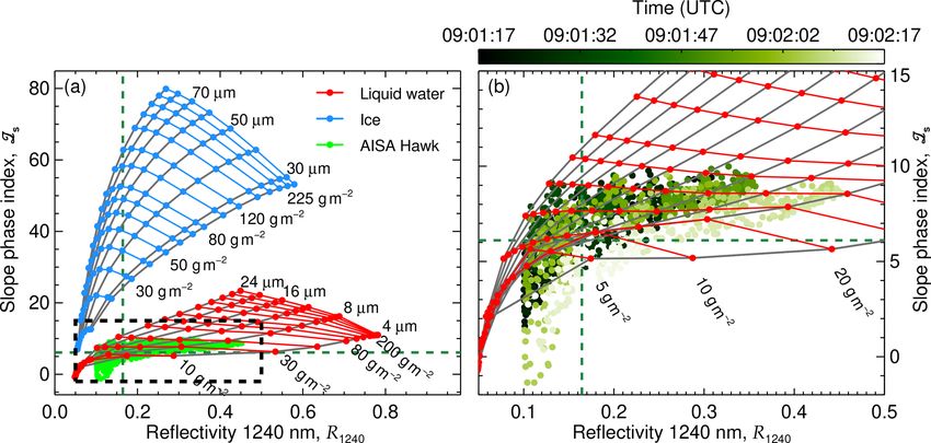
5490                  E. Ruiz-Donoso et al.: Small-scale structure of thermodynamic phase in Arctic mixed-phase clouds

2.2    Radiative transfer modeling                                  tures will cause an overestimation of the optical thickness in
                                                                    the brightly illuminated areas, the effective radius is overesti-
Radiative transfer simulations are employed to interpret the        mated in the shadowed regions. Horváth et al. (2014) showed
horizontal structure of the slope phase index and to retrieve       that, due to their opposite sign, the 3D bias of retrieved opti-
2D fields of cloud optical thickness (τ ) and effective radius      cal thickness and effective radius partially cancel when cal-
(reff ). They were performed with the Library for Radiative         culating the liquid water path (LWP). Therefore, the retrieved
transfer (libRadtran) code (Mayer and Kylling, 2005; Emde           fields of τ and reff are converted into fields of LWP using the
et al., 2016). The simulations applied the radiative trans-         relation by Kokhanovsky (2004):
fer solver FDISORT2 (Discrete Ordinate Radiative Trans-
fer) introduced by Stamnes et al. (2000). The standard sub-                  2
                                                                    LWP =      · ρ · τ · reff .                                  (3)
Arctic summer atmospheric profile provided by libRadtran                     3
was employed, together with temperature and water vapor             As it was the case for the retrieved τ and reff , this conversion
profiles measured by dropsondes released during the re-             assumes liquid water clouds with a homogeneously mixed
spective flights close to the measurement sites. A maritime         vertically constant profile. Considering a homogeneous ver-
aerosol type and the surface albedo of open ocean were se-          tical profile may result in inaccuracies even for pure liquid
lected (Shettle, 1990). The solar zenith angle (SZA) was ad-        water clouds (Zhou et al., 2016). Mixed-phase clouds, in ad-
justed to the location and time of each specific measurement.       dition, violate the pure-phase assumption. The presence of
The simulations of liquid water clouds assumed the validity         ice crystals introduces a significant error in the calculated
of Mie theory, whereas those including ice clouds assumed           LWP, which reaches values well above the typical values ob-
columnar ice crystals and applied the “Hey” parameteriza-           served in Arctic pure liquid water clouds. Past observations
tion, based on Yang et al. (2000) to convert microphysical          show that the LWP of typical Arctic boundary-layer clouds
into optical properties. Regarding the phase index, Ehrlich         is in the range of 30–50 g m−2 and rarely exceeds 100 g m−2
et al. (2008a, b) found that the influence of the ice crys-         (Shupe et al., 2006; Mioche et al., 2017; Nomokonova et al.,
tal shape is of minor importance compared to the impact             2019; Gierens et al., 2020). Appendix A analyzes the dif-
of the particle size, which was confirmed by additional sim-        ferent impact of shades and inhomogeneous thermodynamic
ulations considering different ice crystal habits (not shown        phase distributions in the retrieved LWP. In this paper, un-
here). Hence, the assumption of columns is sufficient to ac-        realistically high retrieved LWP values are used to identify
count for the nonsphericity effects of the ice crystals.            mixed-phase clouds.
   In a first step, extending the work of Bierwirth et al. (2013)
and Schäfer et al. (2013) to the near-infrared spectral range,      2.3   Large eddy simulation (LES)
the spectral cloud top reflectivity fields measured by AISA
Hawk were used to retrieve fields of optical thickness and          Simulations using the ICOsahedral Non-hydrostatic atmo-
effective radius. For this purpose, the reflectivity R1240 at       sphere model (ICON), operated in its large eddy model
a wavelength of 1240 nm (scattering dominated), sensitive           (LEM) configuration (Heinze et al., 2017; Dipankar et al.,
to the cloud optical thickness, is combined with R1625 at           2015), provide a quantitative view into the cloud vertical
a wavelength of 1625 nm, where absorption of solar radia-           structure. The simulated cloud vertical profiles were used as
tion dominates and is influenced mainly by the particle size        input for radiative transfer simulations to analyze the impact
(Nakajima and King, 1990). The location of these wave-              of different vertical distributions of the cloud thermodynamic
lengths in the cloud top reflectivity spectrum are shown in         phase on the cloud top horizontal variability.
Fig. 1. To reduce the retrieval uncertainties, the radiance ratio      ICON-LEM simulations were forced by initial and lateral
approach by Werner et al. (2013) was applied. Look-up tables        boundary conditions from the European Centre for Medium-
considering the sensor viewing geometry of every pixel of           Range Weather Forecasts (ECMWF) Integrated Forecast
AISA Hawk are simulated for various combinations of cloud           System (IFS; Gregory et al., 2010). The simulations were
optical thickness and effective radius. For the simulations,        preformed in a one-way nested setup with a 600 m spatial
pure liquid water clouds are assumed. Therefore, in the case        resolution at the outermost domain, followed by 300 m reso-
of mixed-phase clouds, the retrieved values of optical thick-       lution and an inner triangular nest of 150 m resolution. This
ness and effective radius might be biased. However, since           inner nest was equivalent to a square grid of 100 m horizontal
Arctic low-level mixed-phase clouds are typically topped by         resolution, which is about 1 order of magnitude coarser than
a liquid-water layer (Shupe et al., 2006; McFarquhar et al.,        the observations by AISA Hawk. Simulations with finer hori-
2007), the associated uncertainties are expected to be lower        zontal resolution were not reasonable due to the high compu-
than the variability within the cloud field.                        tational time. In the vertical direction, 150 height levels were
   The retrieved optical thickness and effective radius, as-        simulated. In the ICON-LEM simulations the two-moment,
suming a plane-parallel 1D radiative transfer model, are af-        mixed-phase bulk microphysical parameterization by Seifert
fected by 3D radiative effects (Zinner and Mayer, 2006; Mar-        and Beheng (2006) was applied. It provided vertical profiles
shak et al., 2006). While the 3D nature of the cloud struc-         of liquid and ice mass mixing ratios, rw and ri , cloud droplets

Atmos. Chem. Phys., 20, 5487–5511, 2020                                                 www.atmos-chem-phys.net/20/5487/2020/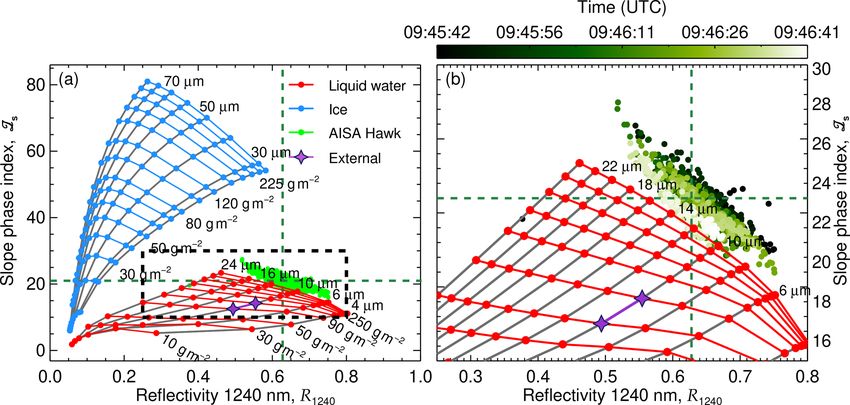
E. Ruiz-Donoso et al.: Small-scale structure of thermodynamic phase in Arctic mixed-phase clouds 5491
Figure 1. Reflectivity spectra of a pure liquid water cloud and a pure ice cloud of optical thickness 12 compared with a clear-sky spectrum
in the wavelength range measured by AISA Hawk. The vertical dashed lines indicate the wavelengths needed to calculate the slope phase
index (1550–1700 nm) and to retrieve the cloud optical thickness (1240 nm) and effective radius (1625 nm).
and ice crystal number concentrations, Nw and Ni , air tem- (30 May–12 June) period, and a neutral (13 June–26 June)
perature T , and pressure p. The mass mixing ratio and the period . During the cold period, the Svalbard region was af-
number concentration profiles take into consideration both fected by a northerly cold air outbreak, which led to the de-
the non-precipitating (cloud water and cloud ice) and the pre- velopment of low-level clouds over the warm open ocean.
cipitating (rain, snow, graupel, and hail) hydrometeors. They Over the Fram Strait, these clouds organized in a roll con-
have been used to convert the rw and ri into liquid water con- vective structure, forming typical cloud streets. During the
tent and ice water content (LWC and IWC), as required by warm period, a high pressure system south of Svalbard ad-
the radiative transfer model as follows: vected warm air from the south over the archipelago, leading
p(z) p(z) to the development of a low-level, optically thick, and ho-
LWC(z) = rw (z) · , IWC(z) = ri (z) · , (4) mogeneous stratocumulus. Cold air outbreaks and warm air
R · T (z) R · T (z)
advections are phenomena often affecting the Arctic regions
with R = 287.06 J kg−1 K−1 the specific gas constant for dry (Pithan et al., 2018; Sedlar and Tjernström, 2017; Woods
air and z the altitude. For the spherical liquid water droplets, et al., 2013; Kolstad et al., 2009; Fletcher et al., 2016). The
vertical profiles of droplet effective radius are obtained by occurrence of both situations during the ACLOUD campaign
(Martin et al., 1994; Kostka et al., 2014): make it an ideal test bed to contrast the characteristics of
1/3 the clouds occurring under each situation. Two cloud cases
3 · rw (z) observed on 25 May, during the cold air outbreak, and on
reff,liquid (z) = , (5)
4 · π · ρw · Nw (z) 2 June 2017, during the warm air advection, were analyzed
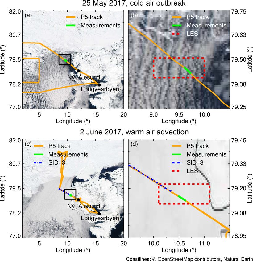
where ρw is the density of the liquid water. For the nonspher- in detail. Figure 2 displays the corresponding MODerate res-
ical ice crystals, the median mass diameter Dm,ice of the par- olution Imaging Spectroradiometer (MODIS) true color im-
ticle size distribution (PSD) of cloud ice represented by the ages showing the clouds on both days.
generalized 0 distribution described by Seifert and Beheng Figure 3 illustrates the combined measurements of
(2006), used by ICON-LEM, is calculated as MiRAC and AMALi for the 1 min sequence acquired over
open ocean for the two cloud cases. The combination of mea-
ri (z) b
surements is interpreted qualitatively to gain an insight into
Dm,ice (z) = a · , (6)
Ni (z) the clouds vertical structure. In both cases, the liquid cloud
top is well identified by the strong backscatter of the lidar
with a = 0.206 × 10⁻⁶ m kg−b and b = 0.302. The radiative signal, defined as in Langenbach et al. (2019) and highly
properties of ice crystals were parameterized using the effec- sensitive to liquid droplets. Whereas on 25 May the liquid
tive radius reff,ice . To convert the median particle size into layer is geometrically thicker, the lidar reaches the surface,
radius reff,ice , the measurement-based relationship between which indicates a cloud optical thickness of less than 3–4
Dm,ice and the effective diameter, Deff,ice , of columnar ice (McGill et al., 2004). On 2 June, the lidar could not pen-
crystals introduced by Baum et al. (2005) and Baum et al. etrate the cloud. The stronger attenuation of the lidar sig-
(2014) was used. nal, i.e., the rapid decrease in the lidar backscatter, hints at
larger amounts of liquid than on 25 May. In contrast, the
3 Results of measurements and radiative transfer radar signal is dominated by larger particles, and higher radar
simulations reflectivity values commonly indicate higher concentrations
of ice crystals. The combination of the radar and lidar signals
The ACLOUD campaign was classified by Knudsen et al. helps to identify differences in the vertical structure of both
(2018) into a cold (23 May–29 May) period, a warm clouds. The cloud on 25 May, showing a high radar reflec-
www.atmos-chem-phys.net/20/5487/2020/ Atmos. Chem. Phys., 20, 5487–5511, 2020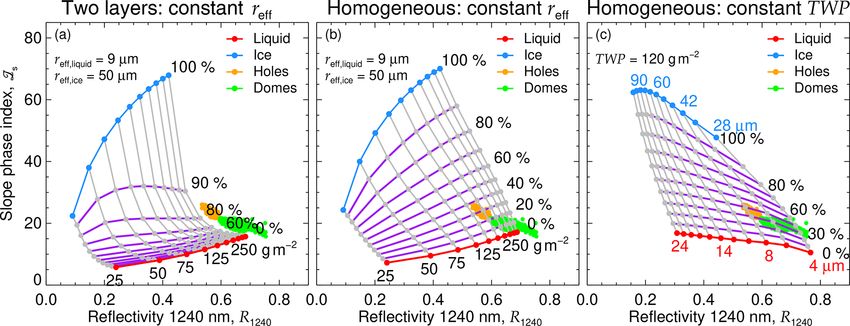
5492                   E. Ruiz-Donoso et al.: Small-scale structure of thermodynamic phase in Arctic mixed-phase clouds

Figure 2. MODIS true color images from the NASA Worldview application (https://worldview.earthdata.nasa.gov, last access: 5 Octo-
ber 2019) on (a) 25 May 2017 during a cold air outbreak and on (c) 2 June 2017 during a warm air advection. Zooms into the regions
delimited by black squares are shown in (b) and (c). The measurements location (79.5◦ N, 9.5◦ E on 25 May and 79.2◦ N, 10.7◦ E on 2 June)
is indicated by the green section of the flight track of Polar 5 (orange). The areas extracted from the LESs are indicated by the dashed red
rectangle. The dashed-dotted blue on 2 June line indicates the location of the SID-3 measurements.

Figure 3. Combination of MiRAC radar reflectivity (color range between blue and red) and AMALi backscatter ratio (colors between white
and black) as measured on (a) 25 May 2017 during a cold air outbreak and on (b) 2 June 2017 during a warm air advection. AMALi’s
lidar backscatter ratio is highly sensitive to the liquid droplets and shows the liquid top layer in both clouds. MiRAC’s radar reflectivity is
dominated by larger particles and indicate regions with ice crystals. The radar signal below an altitude of 150 m is heavily influenced by
ground clutter and cannot interpreted for cloud studies.

Atmos. Chem. Phys., 20, 5487–5511, 2020                                                      www.atmos-chem-phys.net/20/5487/2020/
E. Ruiz-Donoso et al.: Small-scale structure of thermodynamic phase in Arctic mixed-phase clouds 5493
tivity, contains very likely precipitating large ice crystals. In enhanced condensation occurs due to adiabatic cooling (Ger-
this case, some regions of the cloud are characterized by a ber et al., 2005).
large radar reflectivity at cloud top, shown by the overlap- Although Is is always below the threshold of pure ice
ping radar and lidar signals in Fig. 3a, which hints at the clouds, the cloud field presents significant small-scale vari-
presence of large particles in high cloud layers. Vertical sep- ability that might be related to spatial changes in the ther-
aration between the signals of both instruments, such as oc- modynamic phase distribution. To quantify if regions of en-
curring around 09:01:47 UTC, indicate regions where small hanced Is are correlated with areas of precipitating ice crys-
liquid droplets dominate the cloud top, detected by the li- tals, as observed by MiRAC, the cloud edges were separated
dar but not by the radar. In these regions, the radar observes from the central cloud regions. All pixels below the 25th per-
large particles, likely ice crystals, around 100 m below the centile of R1240 and of Is are defined as cloud edges. All
cloud top which precipitate down to the surface. On 2 June other areas are considered to be cloud core center regions.
(Fig. 3b), the radar reflectivity is weaker than on 25 May and The separated measurements were compared to 1D radiative
shows no evidence of precipitation reaching the surface. The transfer simulations adapted to the measurement situation. In
weaker radar reflectivity may be attributed either to smaller Fig. 5, the measured slope phase index is presented as a func-
ice crystals or to a reduced particle concentration. However, tion of the cloud top reflectivity, together with simulations
the continuous overlap between the lidar and the radar signals assuming pure-phase (either liquid or ice) clouds of known
in Fig. 3 indicates the presence of large particles right below particle sizes and liquid/ice water paths (LWPs, IWPs). This
the cloud top. These differences in the vertical structures of sensitivity study shows the spread of Is as a function of
the two cloud cases need to be considered when interpreting the cloud thermodynamic phase, the cloud optical thickness
the 2D horizontal fields of the slope phase index retrieved by (or LWP and IWP), and the cloud particle size. An accurate
AISA Hawk, which is most sensitive to the cloud top layer. phase classification cannot rely on a fixed Is threshold value
and depends on the combined Is and R1240 values. Figure 5
3.1 Cold air outbreak reveals that the observed Is and R1240 range within simulated
values covered by pure liquid water clouds. The spatiotem-
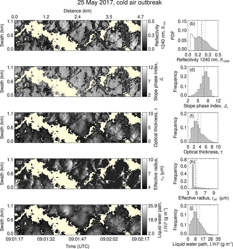
Figure 4 presents a sequence of AISA Hawk measure- poral changes in the measurement (color code in Fig. 5) in-
ments and retrieved horizontal fields of cloud properties dicate that a transition from cloud edge into cloud core fol-
(R1240 , Is , τ , reff , and LWP) together with corresponding his- lows lines with increasing LWP and slightly increasing parti-
tograms. They were observed during the cold air outbreak on cle sizes. This pattern can be explained by the dynamical and
25 May 2017 in the flight section shown in Fig. 2a and b, microphysical processes in cloud cores where ascending air
simultaneously with the MiRAC and AMALi observations condenses and cloud droplets grow with altitude, leading to a
in Fig. 3a. Mean values and associated uncertainty in the higher LWP. Hence, the small-scale variability in Is observed
cloud properties are summarized in Table 1. The measure- on 25 May 2017 can be interpreted as the natural variability
ments present 1 min of data acquired at 09:01 UTC with a of the cloud top liquid layer. Compared to the radar observa-
SZA of 60.5◦ at a flight altitude of 2.8 km. The average cloud tions, the passive reflectivity measurements are insensitive to
top was located at 400 m above sea level. The observed cloud the precipitating ice crystals.
scene covers an area of 1.1 km×4.7 km with an average pixel
size of 3.9 m×2.6 m. Figure 4a shows the cloud top reflectiv- 3.2 Warm air advection
ity field at 1240 nm wavelength, R1240 , and a corresponding
histogram in Fig. 4b. Due to the broken character of the cloud 3.2.1 2D horizontal fields
field, a cloud mask has been applied prior to the retrieval of
cloud properties. Based on radiative transfer simulations, a A sequence of R1240 and retrieved cloud properties (Is , τ ,
threshold of R1240 = 0.1, roughly corresponding to a LWP reff , and LWP) observed in the ACLOUD warm period on
of 2 g m−2 , was chosen to discriminate between cloudy and 2 June 2017 is shown in Fig. 6 for the flight section of
cloud-free areas. Regions with R1240 < 0.1 were classified as Fig. 3b. Table 1 presents the mean values and associated
cloud-free and have been excluded from further analysis. uncertainty in the presented cloud properties. The 1 min se-
The slope phase index Is , presented in Fig. 4c and d, quence starts at 09:45 UTC, when the SZA was of about
shows a maximum value of 12.6, which is characteristic 57.9◦ . The lidar observations indicated that the cloud top of
for pure liquid water clouds. This seems to disagree with the low-level stratocumulus was located at 900 m above sea
the lidar and radar observations (Fig. 3), which indicated a level. Hence, for a flight altitude of 2.9 km, the field covers
mixed-phase cloud, and demonstrates the higher sensitivity a cloud area of 0.9 km × 5.6 km with an average pixel size
of the phase index to the thermodynamic phase of the top of 3.1 m×4.7 m. The cloud top reflectivity at 1240 nm wave-
most layer. Similarly, the LWP (Fig. 4i), calculated from τ length, displayed in Fig. 6a, shows a rather horizontally uni-
(Fig. 4e) and reff (Fig. 4g) using Eq. (3), increases towards form cloud layer compared to the measurements collected on
the cloud core centers, as it is typical for pure liquid water 25 May 2017 (Case I). The cloud mask (R1240 > 0.1) reveals
clouds. These areas visually identify updraft regions where a 100 % cloud coverage for this scene. The slope phase in-
www.atmos-chem-phys.net/20/5487/2020/ Atmos. Chem. Phys., 20, 5487–5511, 2020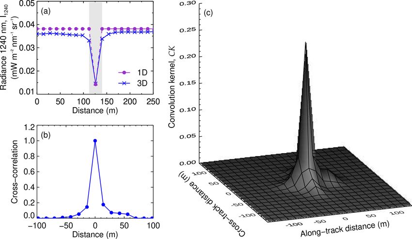
5494                    E. Ruiz-Donoso et al.: Small-scale structure of thermodynamic phase in Arctic mixed-phase clouds

Figure 4. AISA Hawk measurement on 25 May 2017. (a) Cloud top reflectivity, (c) slope phase index, (e) retrieved optical thickness,
(g) retrieved effective radius, and (i) liquid water path. The overlaid contours in (a) and (c) separate the cloud central regions from the cloud
edges. The frequency of occurrence histograms are displayed on the corresponding righthand panels (b), (d), (f), (h), and (j). Data classified
as cloud-free are shown by the non-colored histogram in (b). Dashed lines indicates the mean value of each field, and the dotted lines show
the corresponding 25th and 75th percentiles.

Table 1. Average value and uncertainty (1) in the cloud top properties derived from the measurements of AISA Hawk on 25 May and on
2 June. Independent estimations of the LWP range by the passive 89 GHz channel of MiRAC are also included.

                                                                             25 May 2017          2 June 2017
                                  ztop (m)                                            400                 900
                                  SZA (◦ )                                            60.5               57.9
                                  R̄1240 ± 1R̄1240                            0.23 ± 0.01         0.65 ± 0.03
                                  Īs ± 1Īs                                  7.36 ± 0.04          20.3 ± 1.0
                                  τ̄ ± 1τ̄                                    3.35 ± 0.15          33.7 ± 4.8
                                  r̄eff ± 1r̄eff (µm)                            4.7 ± 1.5         12.5 ± 3.5
                                  LWP ± 1LWP (g m−2 )                           10.3 ± 3.7           271 ± 93
                                  LWPMiRAC ± 1LWPMiRAC (g m−2 )             20 ± 1–40 ± 2     90 ± 5–120 ± 7

Atmos. Chem. Phys., 20, 5487–5511, 2020                                                       www.atmos-chem-phys.net/20/5487/2020/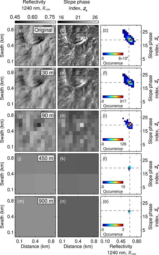
E. Ruiz-Donoso et al.: Small-scale structure of thermodynamic phase in Arctic mixed-phase clouds                                       5495

Figure 5. (a) Is measured on 25 May 2017 presented as a function of R1240 (green dots). The dashed lines indicate the 25th percentile of
R1240 and Is . The two grids represent radiative transfer simulations for a range of pure liquid (red) and pure ice (blue) clouds. The liquid
water clouds cover droplets with reff between 4 and 24 µm and LWP between 1 and 250 g m−2 . The ice clouds are simulated for columnar
ice crystals with reff between 28 and 90 µm and IWP between 1 and 250 g m−2 . A SZA of 60.5◦ was considered. (b) Zoom of the area
highlighted by a dashed rectangle in (a). Color-coded is the acquisition time of the measurements illustrating changes along the flight path.

dex, presented in Fig. 6c, is higher compared to the cloud               particle size distribution observed by the SID-3 (Schnaiter
case presented in Fig. 4 and ranges between 14.9 and 36.5.               and Järvinen, 2019) deployed in Polar 6 between 09:25 and
Applying the common threshold of 20 would classify larger                09:35 UTC in the vicinity of the AISA Hawk measurements
regions of the observed clouds as pure ice or mixed-phase.               (Fig. 2) revealed that, for the observed cloud, the particles
However, the LWP (Fig. 6i) shows significant variability over            at cloud top present effective radii of approximately 10 µm.
the entire cloud field, which may be related to the spatial              Overall, 75 % of the AISA Hawk measurements on 2 June
distribution of the thermodynamic phase. The comparison of               retrieved an effective radii larger than this value (Fig. 6g and
the relation between Is and R1240 with simulations assuming              h). The small-scale variability in the cloud properties shows
pure-phase clouds is shown in Fig. 7. The simulations reveal             that the largest deviation in the retrieved reff and LWP with
that the measurements do not fall in the range of the grid               respect to the external measurements occurs in areas of low
simulated for pure ice clouds, which would typically have                reflectivity (below the 25th percentile of R1240 ) and high
higher values of slope phase index than observed. The mea-               slope phase index values (above the 75th percentile of Is ).
surements rather resemble the simulations of pure liquid wa-             These areas indicate cloud holes, where the vertical velocity
ter clouds. However, the field and histogram of LWP (Fig. 6i             is likely downwards, and the condensation of liquid droplets
and j) show an average value of 270 g m−2 with the 25 %                  is reduced, which increases the fraction of ice crystals. Al-
percentile at 250 g m−2 . Such high LWP values have rarely               though the theory predicts low values of LWP and reff in
been observed in Arctic low-level clouds, which typically                these regions (Gerber et al., 2005, 2013), the high ice frac-
range between 30 and 50 g m−2 and rarely exceed 100 g m−2                tion leads to the strong overestimation of LWP compared to
(Shupe et al., 2005; de Boer et al., 2009; Mioche et al., 2017;          the microwave retrieval. In contrast to the pattern observed
Nomokonova et al., 2019; Gierens et al., 2020). The mea-                 on 25 May 2017, the higher ice fraction in the edges of the
surements by the passive 89 GHz channel of the microwave                 cloud holes causes the slope phase index to decrease with
radiometer of MiRAC were used to estimate the LWP inde-                  increasing cloud top reflectivity.
pendently (see Appendix B for retrieval description and un-
certainty assessment). The values between 90 and 120 g m−2               3.2.2   Impact of the vertical distribution of ice and
indicate that the LWP retrieval using the AISA Hawk mea-                         water
surements is strongly overestimated likely due to the pres-
ence of ice crystals close to cloud top (compare Fig. 3). This           Mixed-phase clouds in the Arctic commonly consist of a sin-
is supported by the rather high optical thickness and particle           gle layer of supercooled liquid water droplets at cloud top,
sizes retrieved from AISA Hawk measurements, shown in                    from which ice crystals precipitate (Mioche et al., 2015),
Fig. 6e–h. As the retrieval assumes liquid droplets, the pres-           which is in line with the radar/lidar observations presented
ence of ice crystals, which are typically larger and strongly            in Fig. 3. Additionally, Ehrlich et al. (2009) found evidence
absorb radiation at 1625 nm wavelength, bias the retrieval of            of ice crystals near the cloud top. Horizontal inhomogeneities
both quantities towards higher values (Riedi et al., 2010). The          in the vertical distribution of the liquid water and ice occur
                                                                         in horizontal scales of 10 m (Korolev and Isaac, 2006; Law-

www.atmos-chem-phys.net/20/5487/2020/                                                      Atmos. Chem. Phys., 20, 5487–5511, 2020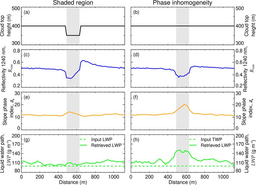
5496                    E. Ruiz-Donoso et al.: Small-scale structure of thermodynamic phase in Arctic mixed-phase clouds

Figure 6. AISA Hawk measurement on 2 June 2017. (a) Cloud top reflectivity, (c) slope phase index, (e) retrieved optical thickness, (g) re-
trieved effective radius, (i) and liquid water path. The overlaid contours in (a) and (c) separate the cloud central regions from the cloud
edges. The frequency of occurrence histograms are displayed on the corresponding righthand panels (b), (d), (f), (h), and (j). The dashed
line indicates the mean value, and the dotted lines show its 25th and 75th percentiles.

Figure 7. (a) Is measured on 2 June 2017 presented as a function of R1240 (green dots). The dashed lines indicate the 25th percentile of
R1240 and the 75th percentile of Is . The two grids represent radiative transfer simulations for a range of pure liquid (red) and pure ice
(blue) clouds. The liquid water clouds cover droplets with reff between 4 and 24 µm and LWP between 1 and 250 g m−2 . The ice clouds are
simulated for columnar ice crystals with reff between 28 and 90 µm and IWP between 1 and 250 g m−2 . A SZA of 57.9◦ was considered.
The purple stars show the independent LWP range retrieved by the 89 GHz passive channel of MiRAC and the SID-3 in situ observation of
particle size. (b) Zoom into the area highlighted by a dashed rectangle in (a). Color-coded is the acquisition time of measurements illustrating
changes along the flight path.

Atmos. Chem. Phys., 20, 5487–5511, 2020                                                      www.atmos-chem-phys.net/20/5487/2020/
E. Ruiz-Donoso et al.: Small-scale structure of thermodynamic phase in Arctic mixed-phase clouds 5497
son et al., 2010) and are expected to relate to the small-scale the 25th percentile of R1240 and phase index below the 75th
structures (i.e., holes and domes) on the cloud top. There- percentile of Is ), where IF is between 0 % and 20 %. Fig-
fore, reproducing the observed trends of R1240 and Is with ure 8c shows the alternative scenario where the TWP is fixed
simulated mixed-phase clouds can provide information about to 120 g m−2 . The simulated clouds cover most of the ob-
the horizontal distribution of the cloud thermodynamic phase served combinations of slope phase indices and reflectivities.
vertical structure. For this reason, the R1240 and Is observed In this scenario, the observed cloud would agree with mixed-
on 2 June are compared with three different vertical mix- phase clouds of fixed IF of about 40 %. In contrast to the
ing scenarios. A two-layer cloud scenario with a layer of scenario with fixed reff , this pattern indicates that the ice frac-
liquid water droplets at cloud top (750–900 m) and a cloud tion in the cloud centers is similar to that in the cloud holes.
bottom layer (600–750 m) consisting of precipitating ice par- The cloud domes centers consist of small droplets with ef-
ticles was assumed to represent the common two-layer verti- fective radii between 4 and 6 µm and small ice crystals with
cal thermodynamic phase distribution. In a second and third effective radii between 28 and 36 µm. Larger droplets, with
scenario, a vertically homogeneous mixture of ice and liq- reff between 6 and 8 µm, and ice crystals, with reff between
uid particles was assumed in the cloud layer (600–900 m), to 36 and 42 µm, are found in the cloud holes. This pattern can
represent the case when both liquid water and ice crystals are be explained by a quick evaporation of small droplets in the
also present in the upper cloud top layer. The partitioning be- cloud holes, leading to a larger reff . Both idealized homo-
tween ice and liquid droplets was varied by changing the ice geneous mixing scenarios reproduce the observations. How-
fraction, defined by ever, based on the AISA Hawk measurements of Is alone,
it cannot be judged which scenario is more likely. In reality,
IWP
IF = · 100 %, (7) neither the particle sizes nor the TWP is horizontally fixed
TWP in a cloud field. A combination of both scenarios might be
with the total water path defined as TWP = LWP + IWP. closest to reality. However, due to the large number of pos-
Pure liquid water clouds correspond to IF = 0 % and pure ice sible realizations (combinations of IWP, LWP, reff,ice , and
clouds to IF = 100 %. The slope phase index and the spectral reff,liquid ), it is impossible for it to fully resemble the obser-
cloud top reflectivity depend on the reff of the ice and liq- vations.
uid particles and on the TWP. To inspect the spread of Is as
a function of R1240 for mixed-phase cases with different IF,
either the reff of the liquid and ice particles or the TWP was 4 Comparison of measurements and LES
kept constant. The approach using a constant value of reff was
Comparing simulated cloud top reflectivities and phase index
evaluated for the two-layer (Fig. 8a) and the vertically homo-
based on ICON-LEM cloud fields with the measurements of
geneous mixing scenarios (Fig. 8b), considering a fixed reff
AISA Hawk will help to evaluate the conclusions about the
of 9 µm for the liquid droplets and 50 µm for the ice crystals.
vertical structure of the cloud thermodynamic phase drawn
The TWP was varied between 25 and 250 g m−2 . The fixed
in the previous section.
TWP approach was evaluated for the homogeneous mixing
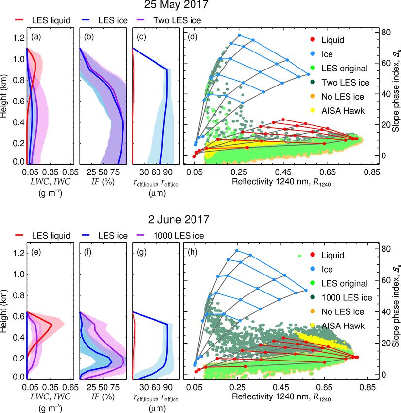
For the two cloud cases of 25 May and 2 June, two re-
scenario (Fig. 8c). Here, the TWP was fixed to 120 g m−2 .
gions of 21 km × 11 km enclosing the corresponding aircraft
In this case, the reff ranges between 4 and 24 µm for liquid
measurements were simulated by ICON-LEM (Fig. 2). The
droplets and between 28 and 90 µm for ice crystals. The three
resulting cloud profiles are shown in Fig. 9a–c and e–g. The
scenarios show grids of Is where the increasing IF yields
profiles of ice fraction IF(z) shown in Fig. 9b and f are cal-
different patterns. The comparison with the measurements
culated, in correspondence to Eq. (7), by
shows that only the homogeneously mixed scenarios (Fig. 8b
and c) may reproduce the measured values of the slope phase IWC(z)
index. In the two-layers scenario (Fig. 8a), the liquid water IF(z) = · 100 %. (8)
LWC(z) + IWC(z)
signature dominates Is , masking the presence of the cloud
ice. These mixed-phase clouds need to be formed of at least On 25 May, the clouds simulated by ICON-LEM are lo-
IF = 70 % to cause phase indices that effectively differ from cated at higher altitudes than observed. However, the sim-
those of pure liquid clouds. Additionally, the TWP required ulated profiles of LWC, IWC, and IF confirm the vertical
to match the observations exceeds the observed values. This cloud structure indicated by the active remote sensing mea-
indicates that a significant amount of ice near the cloud top surements (Fig. 3a), with both liquid and ice phases being
is needed to explain the observed high values of Is . present. The IWC reaches a maximum value of 0.08 g m−3
The homogeneous phase mixing scenario presented in 430 m below the 0.12 g m−3 maximum LWC at 900 m.
Fig. 8b could explain part of the observed values of the reflec- The cloud top reflectivities simulated by libRadtran on the
tivity and slope phase index. According to this scenario, the basis of the clouds simulated by ICON-LEM have been used
cloud holes (reflectivity below the 25th percentile of R1240 ) as synthetic measurements to calculate Is . These synthetic Is
would show higher ice fractions (between 20 % and 40 %) are compared to the observations of AISA Hawk (Figs. 5 and
and higher Is than the cloud dome centers (reflectivity above 7). To further test the sensitivity of R1240 and Is towards the
www.atmos-chem-phys.net/20/5487/2020/ Atmos. Chem. Phys., 20, 5487–5511, 20205498 E. Ruiz-Donoso et al.: Small-scale structure of thermodynamic phase in Arctic mixed-phase clouds Figure 8. Comparison of Is measured on 2 June 2017 as a function of R1240 with three mixing scenarios of mixed-phase clouds. Observations in cloud holes are indicated by orange dots. Green dots represent measurements in cloud domes. Scenario (a) simulates a two-layer cloud, while in scenarios (b) and (c) a homogeneously mixed cloud is assumed. Scenario (b) considers mixed-phase clouds of fixed particle sizes (reff,liquid of 9 µm and reff,ice of 50 µm) and variable TWP between 25 and 250 g m−2 . The grey solid lines connect clouds of equal TWP and the solid purple lines, clouds of equal IF (indicated by the percentages). In scenario (c), TWP is fixed to 120 g m−2 , and the particle sizes are varied. Here, purple lines connect clouds of equal ice fraction, and the grey lines connect clouds considering equal particle sizes. Figure 9. Mean profiles of liquid and ice water content, ice fraction, and effective radius, with (a), (b), and (c) for 25 May 2017 and (e), (f), and (g) for 2 June 2017, respectively. The shaded areas indicate the standard deviation of the considered distribution. The simulated R1240 and Is corresponding to the original LES profiles, as well as simulations neglecting the IWC (“No LES ice”) and modifying it (“Two LES ice” for 25 May and “1000 LES ice” for 2 June), are compared with R1240 and Is of pure-phase clouds and the AISA Hawk measurements in (d) (25 May) and (h) (2 June). Atmos. Chem. Phys., 20, 5487–5511, 2020 www.atmos-chem-phys.net/20/5487/2020/
E. Ruiz-Donoso et al.: Small-scale structure of thermodynamic phase in Arctic mixed-phase clouds 5499
vertical distribution of the cloud thermodynamic phase, addi- 5 Impact of spatial resolution
tional synthetic cloud top reflectivities (firstly, neglecting the
simulated IWC, hence considering pure liquid water clouds, The horizontal resolutions of the ICON-LEM (100 m) and
and secondly, doubling the simulated IWC), were also in- the airborne observations (10 m) differ by about 1 order of
vestigated. The comparisons with the AISA Hawk measure- magnitude. Additionally, satellite-borne imaging spectrome-
ments are shown in Fig. 9d. The relation between R1240 and ters commonly used to derive global distributions of cloud
Is derived from the LES original LWC and IWC profiles properties typically do not reach a spatial resolution as high
shows that the liquid water dominated the cloud top layer, as the AISA Hawk measurements. For instance, the Ad-
making its R1240 and Is indiscernible from those of pure liq- vanced Very High Resolution Radiometer (AVHRR), the
uid water clouds. This is almost identical to the AISA Hawk MODerate resolution Imaging Spectroradiometer (MODIS),
measurements (Fig. 9d). Only a few data points with higher and the Hyperion imaging spectrometer have resolutions of
Is range above the grid of pure liquid water clouds. These 1000, 500, and 30 m pixel sizes, respectively (Kaur and
data mostly have low R1240 and can be linked to cloud edges Ganju, 2008; Li et al., 2003; Thompson et al., 2018). This
with lower LWP located outside the measurement area of raises the question of how much of the observed variability in
AISA Hawk, where ice fractions are simulated to be higher Is is lost by horizontal averaging. To assess this question, the
than observed. Doubling the simulated IWC on 25 May (re- AISA Hawk observations of the two cloud cases were aver-
sulting in a maximum 0.16 g m−2 at 470 m) yielded a similar aged for larger pixel sizes. Figures 10 and 11 show a 900 m×
result; as for the originally simulated profiles, the R1240 and 900 m subsection of the original fields of R1240 and Is pro-
Is relation is for most LES pixels dominated by the higher jected for pixel sizes of 30 m (Hyperion), 90 m (∼ ICON-
liquid water concentration at cloud top and cannot be dif- LEM), 450 m (∼ MODIS), and 900 m (∼ AVHRR). The re-
ferentiated from pure liquid water clouds. However, the en- lationship between Is and R1240 for the complete fields is
hanced IWC increases Is beyond values corresponding to illustrated in Fig. 10c, f, i, l, and o for 25 May 2017 and in
pure liquid water clouds for a larger amount of cloud edge Fig. 11c, f, i, l, and o for 2 June 2017. The statistics of R1240
pixels than with the IWC originally simulated by ICON- and Is corresponding to the considered pixel sizes for both
LEM. days are presented in Table 2.
On 2 June, ICON-LEM produces a maximum IWC The smoothing of the cloud scene with increasing pixel
of 1.5 × 10⁻⁴ g m−3 located 170 m below the maximum size erases the fine spatial structure of the cloud top, which
0.37 g m−3 LWC at 530 m. As for 25 May, the vertical pro- remains only visible for 25 m pixel size. For the cloud case
files of IWC and LWC agree with the active remote sensing of 25 May 2017, the horizontal averaging mainly impacts the
measurements (Fig. 3b), indicating the presence of both liq- observed cloud geometry. The decreasing contrast between
uid and ice. However, as demonstrated by Fig. 9h, the orig- the cloudy and cloud-free pixel changes the cloud mask and
inal IWC simulated by ICON-LEM is too low to effectively eventually causes the loss of the broken cloud nature ob-
impact R1240 and Is , which follow the pattern of pure liquid served by AISA Hawk. The original range of variability in
water clouds and did not reproduce the AISA Hawk observa- R1240 between 0.10 and 0.50 decreases to the range between
tions. This difference suggests that the ICON-LEM underes- 0.14 and 0.23 at 900 m. The original range of Is between
timates the concentration of ice for the cloud on 2 June 2017. −2.12 and 11.7 is reduced to the range from 6.60 to 7.71 but
In a test case, the IWC was increased by a factor of 1000 always indicates a cloud that is dominated by the liquid layer
(maximum value of 1.5 × 10⁻⁴ g m−3 at 360 m) in the same at cloud top. For the cloud on 2 June 2017 (Fig. 11), the av-
order of magnitude as the maximum LWC. For this hypo- eraging cannot affect the 100 % cloud cover. However, the
thetical cloud field, the radiative transfer simulations repro- variability in R1240 becomes significantly reduced for larger
duced the observed values of Is , which deviate from the pure pixel sizes (from the original variability of between 0.18 and
liquid case. However, the results of the ICON-LEM simula- 0.83 to a variability at 900 m of between 0.64 and 0.66) as no
tions show many data points with R1240 way below the ob- large-scale cloud structures are present. Similarly, the vari-
servations (R1240 < 0.45). This indicates that the cloud field ability in Is diminishes for observations with coarser spatial
produced by the LESs, covering a larger area than the obser- resolution from the original range between 15.0 and 36.3 to
vations, presents significant cloud gaps (low TWP), which 19.1 and 19.9 for pixels of 900 m). A coarser resolution re-
were located outside the AISA Hawk measurement region. moves the contrast between cloud holes, which are typically
For the manipulated cloud, these cloud parts show a signif- characterized by the presence of ice crystals (high I s ) and the
icant increase in Is with decreasing R1240 , which can be at- cloud domes, where liquid droplets dominate (lower Is ). For
tributed to cloud edges similar to the cold air outbreak case satellite observations with pixel sizes larger than 90 m, this
of 25 May. prevents the characterization and interpretation of the change
in cloud phase in the small-scale cloud structure and, there-
fore, conceals the information about the vertical distribution
of the thermodynamic phase contained in the cloud top vari-
ability. Highly resolved imaging spectrometer measurements
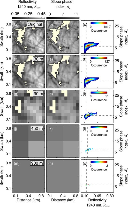
www.atmos-chem-phys.net/20/5487/2020/ Atmos. Chem. Phys., 20, 5487–5511, 20205500 E. Ruiz-Donoso et al.: Small-scale structure of thermodynamic phase in Arctic mixed-phase clouds
Table 2. R1240 and Is dependence upon the sensor resolution.
25 May 2017 2 June 2017
Min. Max. 25th percentile 75th percentile Min. Max. 25th percentile 25th percentile
Original 0.10 0.50 0.16 0.28 0.18 0.83 0.63 0.68
30 m 0.10 0.48 0.16 0.28 0.45 0.76 0.63 0.68
R1240 90 m 0.10 0.42 0.16 0.28 0.51 0.72 0.63 0.67
450 m 0.13 0.33 0.17 0.22 0.63 0.67 0.64 0.66
900 m 0.14 0.23 0.15 0.20 0.64 0.66 0.64 0.65
Original −2.12 11.7 6.54 8.29 15.0 36.3 19.1 21.0
30 m 0.07 9.90 6.60 8.23 16.5 29.8 19.3 20.9
Is 90 m 3.45 9.43 6.62 8.08 17.7 25.0 19.5 20.7
450 m 5.54 8.15 6.94 7.67 19.0 20.9 19.3 20.4
900 m 6.60 7.71 6.77 7.13 19.1 19.9 19.5 19.7
such as the Hyperion and the ICON-LEM, with pixels below ity in Is observed on 25 May relates mostly to the variabil-
100 m are still able to resolve part of the natural horizontal ity in the liquid cloud layers. On 2 June, AISA Hawk mea-
variability. sured higher Is , which hints at the presence of ice crystals
in higher cloud layers. Additionally, the LWP, retrieved by
assuming pure liquid clouds, shows unrealistically high val-
6 Conclusions ues compared to the observations by MiRAC, which supports
this conclusion. The high values of Is and the large retrieval
Based on airborne active and passive remote sensing con- bias of LWP are observed close to areas of low cloud re-
ducted by a passive imaging spectrometer and vertically re- flectivity (cloud holes). The comparison of both cloud cases
solving instruments, such as lidar and radar, the horizontal highlights the limitations of passive remote sensing alone to
and vertical structure of the thermodynamic phase in Arctic identify layered mixed-phase structures if the ice is not suffi-
mixed-phase cloud cases was characterized for two example ciently close to the cloud top. In particular in these cases, the
clouds observed during a cold air outbreak and a warm air combination of active and passive remote sensing is crucial
intrusion event. While the spectral imaging was used to iden- to fully characterize the horizontal and vertical distribution
tify the structure of the horizontal distribution of the cloud ice of ice and liquid water particles in mixed-phase clouds.
at scales down to 10 m, the combined radar and lidar obser- The highly resolved horizontal distribution of Is observed
vations revealed the general vertical thermodynamic phase on 2 June was analyzed using radiative transfer simulations
distribution of the clouds. assuming different mixing scenarios of ice and liquid water
The two cloud cases were observed over open ocean close content. Two homogeneous mixing scenarios, either keep-
to Svalbard (Spitzbergen) during the ACLOUD campaign. ing the TWP or the particle sizes fixed when changing the
The cloud scene sampled on 25 May 2017 evolved within a ice fraction, did reproduce the observed pattern of variabil-
cold air outbreak, whereas a cloud that had formed in a warm ity. However, based on the AISA Hawk measurements of Is
air advection event was sampled on 2 June 2017. For both alone, it cannot be judged which scenario is closer to re-
cloud cases, the combined radar and lidar observations in- ality. To consider modeled phase-mixing scenarios of IWP,
dicated the mixed-phase character of the clouds, with liquid LWP, reff,ice , reff,liquid , and the vertical cloud structure, the
water droplets in the cloud top layer and ice crystals below. ICON-LEM was applied. The microphysical profiles sim-
While the lidar penetrated the strongly reflecting liquid cloud ulated by ICON-LEM roughly represent major features of
layer on 25 May, partly until the surface, the strong extinction the vertical profiles obtained by MiRAC and AMALi for
of the lidar signal close to the cloud top observed on 2 June both cloud cases. To compare with the AISA Hawk measure-
indicates higher liquid water amounts. The vertical structure ments, radiative transfer simulations of the cloud top were
of the radar backscatter also differs between both days, with performed on the basis of the ICON-LEM thermodynamic
reflectivities reaching the ground on 25 May typical for light phase profiles. For both cases, the variability in Is calcu-
snow precipitation. These different cloud vertical structures lated from the simulations is represented by pure liquid water
influenced the ability to detect the ice by the imaging spec- clouds. Enhancing the IWC simulated by ICON-LEM indi-
trometer observations of AISA Hawk using the slope phase cates that, whereas on 25 May this behavior is due to the
index Is . On 25 May, Is is dominated by the liquid water liquid-water-dominated cloud top layer, on 2 June, the sim-
contained at the cloud top layer, which leads to a misclassifi- ulated concentration of ice crystals is underestimated. In a
cation as a pure liquid water cloud. The small-scale variabil- test case where the IWC was enhanced 1000 times, the sim-
Atmos. Chem. Phys., 20, 5487–5511, 2020 www.atmos-chem-phys.net/20/5487/2020/You can also read


