Identifying recharge under subtle ephemeral features in a flat-lying semi-arid region using a combined geophysical approach - HESS
←
→
Page content transcription
If your browser does not render page correctly, please read the page content below
Hydrol. Earth Syst. Sci., 24, 4353–4368, 2020
https://doi.org/10.5194/hess-24-4353-2020
© Author(s) 2020. This work is distributed under
the Creative Commons Attribution 4.0 License.

Identifying recharge under subtle ephemeral features in a flat-lying
semi-arid region using a combined geophysical approach
Brady A. Flinchum1 , Eddie Banks2 , Michael Hatch2,3 , Okke Batelaan2 , Luk J. M. Peeters1 , and Sylvain Pasquet4
1 Commonwealth    Scientific Industrial Research Organization (CSIRO), Deep Earth Imaging Future Science Platform &
Land and Water, Urrbrae, 5064, Australia
2 National Centre for Groundwater Research and Training, College of Science and Engineering,

Flinders University, Adelaide, 5001, Australia
3 Department of Geosciences, School of Physics, University of Adelaide, Adelaide, Australia
4 Université de Paris, Institut de physique du globe de Paris, CNRS, 75005 Paris, France

Correspondence: Brady A. Flinchum (brady.flinchum@csiro.au)

Received: 25 October 2019 – Discussion started: 2 January 2020
Revised: 9 June 2020 – Accepted: 19 June 2020 – Published: 9 September 2020

Abstract. Identifying and quantifying recharge processes          1   Introduction
linked to ephemeral surface water features is challenging
due to their episodic nature. We use a combination of well-
established near-surface geophysical methods to provide evi-      Understanding groundwater recharge mechanisms and
dence of a surface and groundwater connection under a small       surface-water–groundwater connectivity is crucial for sus-
ephemeral recharge feature in a flat, semi-arid region near       tainable groundwater management (Banks et al., 2011; Brun-
Adelaide, Australia. We use a seismic survey to obtain P-         ner et al., 2009). In semi-arid areas, recharge has been shown
wave velocity through travel-time tomography and S-wave           to occur in focused regions beneath perennial streams and
velocity through the multichannel analysis of surface waves.      lakes, and ephemeral streams and ponds (Cuthbert et al.,
The ratios between P-wave and S-wave velocities are used to       2016; Scanlon et al., 2002, 2006). However, identifying lo-
calculate Poisson’s ratio, which allow us to infer the position   calized regions of groundwater recharge remains challeng-
of the water table. Separate geophysical surveys were used        ing.
to obtain electrical conductivity measurements from time-             Many aquifers in semi-arid areas receive a significant por-
domain electromagnetics and water contents from down-             tion of their recharge from adjacent mountain ranges (Bres-
hole nuclear magnetic resonance. The geophysical observa-         ciani et al., 2018; Earman et al., 2006; Wilson and Guan,
tions provide evidence to support a groundwater mound un-         2004; Winograd et al., 1998). In this common scenario,
derneath a subtle ephemeral surface water feature. Our re-        recharge can occur via groundwater flow from the moun-
sults suggest that recharge is localized and that small-scale     tain range directly into the aquifer – implying a significant
ephemeral features may play an important role in ground-          lateral groundwater connection with the adjacent mountain
water recharge. Furthermore, we show that a combined geo-         range (Markovich et al., 2019). Alternatively, precipitation
physical approach can provide a perspective that helps shape      from the mountain range flows out and across the semi-arid
the hydrogeological conceptualization of a semi-arid region.      basin as surface water and recharges the aquifer via river in-
                                                                  filtration processes – implying a vertical connection between
                                                                  surface and groundwater (Bresciani et al., 2018; Brunner et
                                                                  al., 2009; Winter et al., 1998).
                                                                      Groundwater recharge processes span a wide range of spa-
                                                                  tial and temporal scales making them difficult to quantify
                                                                  (Scanlon et al., 2002). Recharge rates are traditionally quan-
                                                                  tified using physical, tracer, or modelling techniques (Scan-

Published by Copernicus Publications on behalf of the European Geosciences Union.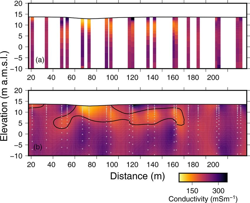
4354           B. A. Flinchum et al.: Identifying recharge under subtle ephemeral features in flat-lying semi-arid region

lon et al., 2002). Physical techniques include carefully mea-      Kotikian et al., 2019) and can highlight preferential flow
suring fluxes and evapotranspiration along various reaches         paths. These methods are still handicapped by the fact that
of a river or stream (Abdulrazzak, 1995; Lamontagne et             they still require the burial or setup of the geophysical equip-
al., 2014), by calculating aquifer water level response times      ment prior to a natural recharge (Kotikian et al., 2019; Thayer
(e.g. water table fluctuation method) (Cuthbert et al., 2019),     et al., 2018) or a man-made event (Carey and Paige, 2016;
or through stream hydrograph separation (Banks et al., 2009;       Claes et al., 2019). It is still challenging to find a suitable geo-
Chapman, 1999; Cuthbert et al., 2016). Common tracer tech-         physical approach that can be deployed rapidly (that is, with-
niques include the use of stable isotopes of hydrogen and          out a time-lapse setup) to determine whether an ephemeral
oxygen (Lamontagne et al., 2005; Taylor et al., 1992; Wino-        drainage feature is acting as a groundwater recharge feature.
grad et al., 1998), quantifying chemical signatures that have         The aim of this study is to use a combination of well-
accumulated from past human activities (e.g. chlorofluoro-         established near-surface geophysical methods to provide ev-
carbons and sulfur hexafluoride) (Cook et al., 1996), and          idence of a surface and groundwater connection of a small,
measuring environmental tracers such as chloride (Allison          shallow, and subtle ephemeral feature in a low-lying semi-
et al., 1990; Anderson et al., 2019; Crosbie et al., 2018)         arid landscape without time-lapse measurements. We used a
and radon (Bertin and Bourg, 1994; Genereux and Hemond,            single seismic survey to obtain P-wave velocity through seis-
2010; Hoehn and Gunten, 1989). Lastly, numerical mod-              mic refraction tomography (SRT) (Sheehan et al., 2005; Zelt
elling is used to estimate recharge over global scales (Glee-      et al., 2013) and S-wave velocity through the multichannel
son et al., 2012; Scanlon et al., 2006) and test existing hydro-   analysis of surface waves (MASWs) (Park et al., 1999; Pas-
geological conceptualizations (Xie et al., 2014).                  quet and Bodet, 2017) to calculate Poisson’s ratio, which al-
   Quantifying recharge processes in ephemeral ponds or            lowed us to infer the position of the water table. A separate
streams in semi-arid regions is particularly difficult because     survey was used to obtain bulk electrical conductivity mea-
flooding events are episodic (Shanafield and Cook, 2014).          surements from transient electromagnetics (TEMs) (Paras-
The infrequency and variable size of flooding events makes         nis, 1986; Reynolds, 2011; Telford et al., 1990). Water con-
it difficult to monitor, quantify, or even identify whether        tents and T2 relaxation times (time constant for the decay
groundwater recharge has occurred. Furthermore, infiltration       of transverse magnetization) were acquired using downhole
is a different process than recharge. Groundwater recharge         nuclear magnetic resonance (NMR) (Walsh et al., 2013). We
must be confirmed by a response in the water table, whereas        used this combination of standard geophysical measurements
water that has infiltrated might have been taken up by             to show that small-scale ephemeral features are likely to con-
vegetation or lost to evaporation. Larger ephemeral rivers         tribute to the localized replenishment of groundwater in shal-
flood frequently so equipment can be installed and be ready        low unconfined aquifers in this low-lying semi-arid environ-
when an event occurs (Dahan et al., 2007, 2008). On the            ment.
other hand, it is more difficult to capture recharge events of
smaller ephemeral tributaries; as a result, the recharge mech-
anisms of these features are less understood. These smaller-       2   Site description
scale features are common on Earth’s surface. It has been
shown that 69 % of first-order streams and ∼ 34 % of larger        The North Adelaide Plains (NAP) are located north of the
fifth-order rivers below 60◦ latitude are ephemeral (Acuña         city of Adelaide, Australia, and are part of the St Vincent
et al., 2014; Raymond et al., 2013). Thus, even if small           Basin, a geological basin underlying the area between the
ephemeral features only provide small amounts of ground-           Yorke Peninsula and the Mount Lofty Ranges in South Aus-
water recharge during individual events, their large spatial       tralia (Fig. 1). The St Vincent Basin is a north–south-trending
distribution means that they could be important to recharge        basin that is characterized by low topographic relief between
processes of a given region.                                       0 and 200 m elevation above sea level (Smith et al., 2015).
   Small ephemeral features are an ideal target for near-          The NAP are bound by the Mount Lofty Ranges to the east
surface geophysical surveys. A wide range of existing and          and their northern boundary is marked by the Light River
standardized geophysical techniques have been used in hy-          (Fig. 1). Land-use in the NAP is predominantly dryland agri-
drological studies (e.g. Robinson et al., 2008; Siemon et          culture with mixed farming (sheep and rotational cropping
al., 2009; Parsekian et al., 2015). To highlight surface and       of wheat, barley, and canola) (Goyder Institute for Water Re-
groundwater connections, geophysical methodologies com-            search, 2016). Potential evaporation is high and the average
monly rely on time-lapse measurements. This is because the         rainfall is low, averaging around 445 mm yr−1 , with an av-
infiltration of groundwater causes changes in geophysical          erage daily temperature of 21.6 ◦ C (Bresciani et al., 2018).
properties on the order of days or months (i.e. the geology        The combination of low rainfall and high evaporation rates
stays constant). Time-lapse electrical resistivity measure-        in the NAP implies that the source water in the aquifers is
ments have been used to observe and monitor recharge path-         from the Mount Lofty Ranges, where the average rainfall
ways (Carey and Paige, 2016; Singha and Gorelick, 2005;            is 983 mm yr−1 (Bresciani et al., 2018). Rainfall is winter-
Johnson et al., 2012; Valois et al., 2016; Thayer et al., 2018;    dominated (May to August), which suggests that recharge is

Hydrol. Earth Syst. Sci., 24, 4353–4368, 2020                                        https://doi.org/10.5194/hess-24-4353-2020
B. A. Flinchum et al.: Identifying recharge under subtle ephemeral features in flat-lying semi-arid region 4355
been shown on the basis of multiple lines of evidence that
water flows from the Mount Lofty Ranges onto the NAP
through ephemeral rivers and streams and recharges the un-
derlying aquifers via vertical infiltration (Bresciani et al.,
2018). In this conceptual model, recharge is mostly localized
and occurs along the main rivers and streams. This concep-
tual model is supported by lower groundwater chloride con-
centrations surrounding Gawler River and Little Para River
in both the Quaternary and Tertiary aquifers and the piezo-
metric surfaces that show groundwater moving away from
the rivers (losing river conditions) and into the underlying
aquifers (Bresciani et al., 2018). Prior to this study, it was
argued that the aquifers of the NAP were recharged through
a lateral groundwater connection with the rocks underlying
the Mount Lofty Ranges. This concept was supported by an
increase in groundwater ages away from the Mount Lofty
Ranges and stable isotopes indicating some evaporation prior
to infiltration (Batlle-Aguilar et al., 2017). It is important to
note that the age and isotope data support the mountain front
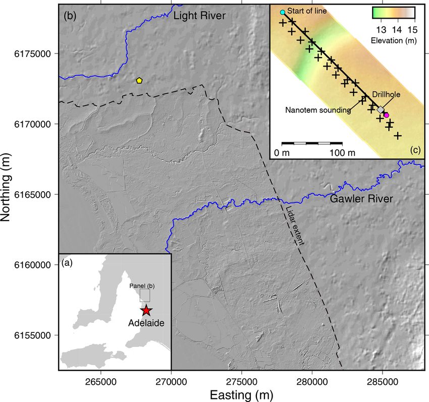
Figure 1. (a) Inset map showing the general location of the study
recharge conceptual model of Bresciani et al. (2018) equally
area relative to the city of Adelaide, South Australia. (b) Hill-shaded well.
topographic relief with the lidar data overlaid. The northern extent Our study site is located on a private farm, 44 km north-
of high-resolution lidar DEM data is marked with a dashed line. west of Adelaide, and is between the Light and Gawler rivers
The yellow star represents the site location. The Light and Gawler (Fig. 1). In May of 2018, as part of a regional study of the
Rivers are shown in blue. (c) High-resolution topography (drone shallow water table, 47 shallow holes were drilled across
based) of the field area where the geophysical testing took place. the northern region of the NAP with a small truck-mounted
The thick black line is the seismic line, where the cyan dot is the Rockmaster drill rig (Hatch et al., 2019). We used these pre-
start and the magenta dot is the end. Black crosses represent the existing sites to select a location where we knew the water
location of NanoTEM soundings. The grey square is the shallow table was within a range of 3–10 m to increase the likelihood
drill hole location and also where the downhole NMR data were
of imaging the water table with the seismic data. The existing
collected.
drill hole would also provide ground-truthing to the geophys-
ical data. Thus, our study transect for the near-surface geo-
physical surveys was located adjacent to one of these drill
also seasonal (Batlle-Aguilar et al., 2017; Bresciani et al., hole sites where we had manual water level measurements,
2018). soil samples, and downhole NMR logs. The 235 m long tran-
Lidar of the NAP shows that within this low-relief land- sect line was positioned so that it crossed a small ephemeral
scape there are many small ephemeral surface drainage fea- topographic feature that is only visible on a map with high-
tures (Fig. 1). These subtle drainage features are visible in resolution elevation data collected via drone (Fig. 1c).
the hill-shaded lidar and indicate that surface water runoff is
likely to flow towards these ephemeral drainage features and
toward the larger streams after precipitation events (Fig. 1b). 3 Methods
These ephemeral features are not monitored because they fall
below the resolution of the 30 m Shuttle Radar Topography To aid in geophysical interpretation and reduce ambiguities,
Mission (SRTM) elevation data (Fig. 1b). The near-surface it is important to “ground-truth” near-surface geophysical
Quaternary aquifers are typically used for stock and do- data with drilling results (Flinchum et al., 2018; Gottschalk
mestic purposes and have salinity ranges between 2000 and et al., 2017; Orlando et al., 2016; West et al., 2019) or to
13 000 mg L−1 (Department for Water, 2010; Goyder Insti- corroborate them by other independent geophysical measure-
tute for Water Research, 2016). The near-surface aquifers are ments. In this study, we combined hydrogeological obser-
only monitored because they present a risk of waterlogging vations with multiple geophysical measurements to obtain
and soil salinization (Department for Water, 2010). different geophysical parameters, specifically bulk electri-
Most of the water that recharges the NAP aquifers comes cal conductivity from TEM, P-wave velocity from SRT, S-
from the Mount Lofty Ranges to the east, supported by the wave velocity from MASW, and water contents from down-
fact that in between streams you find high-salinity water, hole NMR. In April 2018, the shallow drill hole was logged
which suggests the occurrence of diffuse recharge – see the with a downhole NMR system (Vista Clara Dart) and the
conceptual model in Bresciani et al. (2018; Fig. 14). It has water level was measured by hand. Only a week after the
https://doi.org/10.5194/hess-24-4353-2020 Hydrol. Earth Syst. Sci., 24, 4353–4368, 2020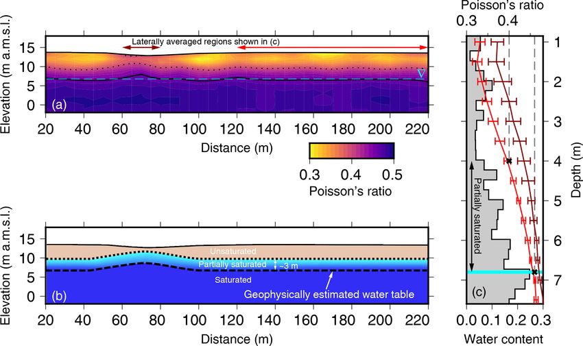
4356           B. A. Flinchum et al.: Identifying recharge under subtle ephemeral features in flat-lying semi-arid region

seismic data were collected, a separate campaign was car-          shots were stacked at each of the 80 locations. The travel
ried out to collect 26 TEM soundings along the same profile        times were picked manually (Figs. S1 and S2 in the Sup-
(Fig. 1c). In this paper, we use these geophysical methods to      plement) and inverted for P-wave velocity using the refrac-
infer a surface-water–groundwater connection without time-         tion module in the Python Geophysical Inversion and Mod-
lapse measurements. In this section we briefly describe the        eling Library (pyGIMLi) (Rücker et al., 2017). The forward
theory behind the geophysical methods and how the mea-             model is based on the shortest path algorithm (Dijkstra, 1959;
surements are influenced by various hydrological properties.       Moser, 1991; Moser et al., 1992). PyGIMLi utilizes a deter-
Additional figures and details pertaining to the processing of     ministic Gauss–Newton inversion scheme and incorporates a
the geophysical data set can be found in the Supplement.           data weight matrix (Rücker et al., 2017). We populated the
                                                                   data weight matrix using reciprocal travel times (Fig. S2).
3.1    Topography acquisition                                      To initialize the inversion, we used a gradient model that
                                                                   had a velocity of 0.4 km s−1 at the surface and 2 km s−1 at
At our study site, no lidar imagery was available. High-           a depth of 40 m. To quantify uncertainty, we incorporated a
resolution imagery of the small study area (∼ 9 ha) was thus       bootstrapping algorithm on the travel-time picks (details in
acquired with a DJI Phantom 4 Pro unmanned aerial ve-              the Supplement). The model fits are determined by a χ 2 mis-
hicle (UAV). The UAV flew a grid pattern over the study            fit, which incorporates our picking errors and an rms error
area at an elevation of 30 m a.g.l. (above ground level) and       (details in Supplement).
collected a photo data set of 834 images. Georeferencing
was undertaken using a Trimble R10 global positioning sys-         3.3   Multichannel analysis of surface waves
tem (GPS) real-time kinematic (RTK) survey with 65 ground
control points located within the study area and provided          At the Earth’s surface, most of the elastic energy travels
a georeferencing root mean square error (rms) of 0.153 m.          as surface waves. Surface waves are the largest amplitude
The captured photos were processed using the photogramme-          events that are recorded in both active source seismic acqui-
try Pix4D software package (Pix4Dmapper Pro version 3.2,           sition and earthquake records. Surface waves are caused by
2017) to generate a high-resolution (0.8 cm per pixel) digital     interactions of the body waves (P waves and S waves) and
surface model (DSM). As the study area was a fallow field at       the boundary conditions that only exist at the surface (Stein
the time of the survey, the DSM was treated as a digital eleva-    and Wysession, 2003). There are two types of surface waves:
tion model (DEM) as there was very little vegetation present.      Love waves and Rayleigh waves (for a detailed review on
The generated DEM was re-sampled to a 0.5 m DEM (Fig. 1)           surface waves, the reader is referred to Stein and Wysession,
that was used to extract the elevation profile along the geo-      2003, and Lowrie, 2007). In this study we take advantage of
physical transect.                                                 the dispersive nature of Rayleigh waves (Park et al., 1999;
                                                                   Pasquet and Bodet, 2017; Xia et al., 1999, 2003). Further-
3.2    Seismic refraction tomography                               more, Rayleigh waves propagate at velocities mostly driven
                                                                   by the S-wave velocity of the medium. The dispersion of
Seismic refraction is an active source geophysical method          Rayleigh waves can be measured by picking the phase ve-
that estimates seismic velocity. A seismic refraction survey       locity as a function of frequency (Park et al., 1999; Xia et
provides a spatial distribution of P-wave velocity (energy         al., 2003). The phase velocity of lower frequencies (longer
propagating along the direction of travel). In a shallow seis-     wavelengths) will be influenced by deeper S-wave velocity
mic refraction survey, the time taken for the energy to travel     structures, whereas higher frequencies will be influenced by
from a source to each individual receiver, called a travel time,   shallower structures. These frequency-dependent phase ve-
is measured. The subsurface velocity structure controls the        locities can then be inverted for one-dimensional (1D) S-
travel times so they can be inverted to retrieve the subsur-       wave velocity models at low computational costs (Pasquet
face P-wave velocity structure using a forward model and an        and Bodet, 2017).
inversion scheme (Sheehan et al., 2005; Zelt et al., 2013).           In this study, we use the acquisition setup from the refrac-
P-wave velocity is controlled by the elastic properties of         tion survey to analyse the dispersion of surface wave energy.
the material, porosity, and saturation (Berryman et al., 2002;     This approach produces a pseudo two-dimensional (2D) sec-
Hashin and Shtrikman, 1963). If the pore space is filled with      tion comprised of 41 1D S-wave velocity profiles, spaced ev-
a fluid, in our case water (regardless of salinity), then the      ery 5 m starting at 17.5 m from the start of the profile. To
P-wave velocity is greater than if the pore space is not filled    build the pseudo 2D profile we used the Surface Wave In-
with fluid (Bachrach and Nur, 1998; Desper et al., 2015; Gre-      version and Profiling (SWIP) package (Pasquet and Bodet,
gory, 1976; Nur and Simmons, 1969).                                2017). First, the seismic data are resorted and windowed to
   In this survey, we used 48 geophones spaced at 5 m, which       sample 1D vertical slices of the subsurface. Once windowed,
produced a 235 m long profile. The source was a 40 kg accel-       the sorted seismic data are transformed into the frequency-
erated weight, striking a 20 cm × 20 cm × 2 cm steel plate at      phase velocity domain using a slant stack (Mokhtar et al.,
every geophone. To increase the signal-to-noise ratio, eight       1988). To increase the depth of investigation, similar disper-

Hydrol. Earth Syst. Sci., 24, 4353–4368, 2020                                       https://doi.org/10.5194/hess-24-4353-2020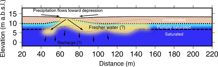
B. A. Flinchum et al.: Identifying recharge under subtle ephemeral features in flat-lying semi-arid region                   4357

sion curves from different shots are stacked together (Ne-         3.5   Nuclear magnetic resonance
ducza, 2007). Once the dispersion curves are constructed
they are picked and an uncertainty associated with each pick       Nuclear magnetic resonance (NMR) capitalizes on the ex-
is defined (O’Neil, 2003) (Fig. S4). To construct our disper-      istence of a measurable magnetic moment produced by the
sion curves, we used 40 m windows (eight stations) and en-         rotation of hydrogen protons contained in water molecules.
sured a 5 m offset between the source and first channel to         At equilibrium, the direction of the magnetic moment points
avoid near-source effects. The picks and corresponding un-         in the direction of a background magnetic field. An NMR
certainty for each windowed dispersion curve are inverted          measurement emits an electromagnetic pulse at a specific fre-
using a Monte Carlo approach and the neighbourhood al-             quency (called Larmor frequency) in order to force protons
gorithm (Sambridge, 1999; Wathelet et al., 2004). We ran           out of equilibrium. When the excitation pulse ends, the pro-
15 000 inversions for each of our dispersion curves and av-        tons return to equilibrium in a process called relaxation. Dur-
eraged the 1000 best-fitting S-wave velocity models to build       ing relaxation, a measurable resonating magnetic moment
final 1D models (Fig. S5) every 5 m (more details about pro-       that decays exponentially can be measured (Bloch, 1946;
cessing can be found in the Supplement). Finally, the indi-        Brownstein and Tarr, 1979; Torrey, 1956). The initial mag-
vidual 1D S-wave profiles are combined into a pseudo-2D            nitude of the signal is directly proportional to the number
section (Pasquet et al., 2015a, b; Pasquet and Bodet, 2017).       of protons excited, which in near-surface exploration come
                                                                   mostly from groundwater, and the rate of decay (i.e. the re-
3.4   Poisson’s ratio                                              laxation time T2 ) is related to the pore size. Thus, NMR
                                                                   has the ability to directly measure the amount of groundwa-
Locating the water table of the unconfined aquifer over large      ter within its measurement volume. For a thorough review
spatial scales is challenging and is traditionally done by         of NMR theory, the reader is referred to Behroozmand et
drilling down to the water table and interpolating manual wa-      al. (2015) and textbooks dedicated to the theory of NMR
ter level measurements between drill hole locations. Building      (Coates et al., 1999; Dunn et al., 2002; Levitt, 2001).
a detailed water table map requires many measurements and             The decay rate, described by T2 , is a function of two dis-
can be limited by logistical or financial constraints. Here, we    tinct processes: the bulk relaxation and the surface relaxation
exploit the fact that P-wave velocities increase when a mate-      (Brownstein and Tarr, 1979; Cohen and Mendelson, 1982;
rial is saturated and the S-wave velocities remain relatively      Grunewald and Knight, 2012). The surface relaxation is con-
unchanged (Bachrach and Nur, 1998; Desper et al., 2015;            trolled by an intrinsic property called the surface relaxivity
Gregory, 1976; Nur and Simmons, 1969).                             and the surface-to-pore volume ratio. Surface relaxivity de-
   Poisson’s ratio is a unitless elastic property that describes   scribes a material’s ability to intensify relaxation. The de-
how much a material will deform in the direction perpen-           pendence on the surface-to-pore volume ratio is what re-
dicular to an applied stress. Poisson’s ratio can be calculated    lates the NMR decay to the pore scale properties. In gen-
from P-wave and S-wave velocities (Eq. 1).                         eral, materials with larger pore spaces have longer T2 relax-
                                                                   ation times (e.g. gravels) and materials with smaller pores
   Vp2 − 2Vs2
υ=                                                        (1)    have shorter T2 (e.g. clays). When high-quality data are ac-
  2 Vp2 − Vs2                                                      quired, such as with downhole systems, the T2 relaxation
                                                                   times can be fit using multi-exponential decay curves. The
In Eq. (1), Vp is P-wave velocity, Vs is S-wave velocity, and      distribution of decay times represents the properties of all
υ is Poisson’s ratio. Poisson’s ratio for geologic materials       the pores within the excited volume. We acquired downhole
ranges from 0 to 0.5. Poisson’s ratio increases as fluid sat-      NMR measurements at 0.25 m depth intervals down a 7.5 m
uration increases (Bachrach et al., 2000; Dvorkin and Nur,         drill hole using a Dart system (Vista Clara). The Dart quanti-
1996; Nur and Simmons, 1969; Salem, 2000). Furthermore,            fies water content and T2 decay times in two cylindrical shells
Poisson’s ratio is an indicator for determining the difference     of varying radii (12.7 and 15.2 cm) within the drill hole.
between gas and fluid saturated materials (Gregory, 1976;
Pasquet et al., 2016) and has been shown to be useful to track     3.6   Transient electromagnetics (TEM)
pressure changes (Prasad, 2002), map the water table depth
(Bachrach et al., 2000; Pasquet et al., 2015a; Salem, 2000;        The transient electromagnetic method utilizes a transmitting
Uyanık, 2011), and differentiate gas and fluid in hydrother-       and receiving loop lying on the earth’s surface. The TEM
mal systems (Pasquet et al., 2016). To image the water ta-         method specifically uses a short-transmitted pulse duration
ble with Poisson’s ratio, the conceptual model of the geology      and measures the decay amplitude of the vertical component
must be simplified (i.e. no lateral changes) and requires that     of the electromagnetic field generated by secondary currents
there are at least a few metres of unsaturated sediments over-     as a function of time. The magnitude and decay rate of the
lying the saturated region to generate a vertical contrast in      vertical electromagnetic field is related to the electrical con-
elastic properties; our study site satisfies both these condi-     ductivity of the subsurface beneath the loop. The penetration
tions.                                                             depth of the method depends on the underlying conductivity

https://doi.org/10.5194/hess-24-4353-2020                                       Hydrol. Earth Syst. Sci., 24, 4353–4368, 2020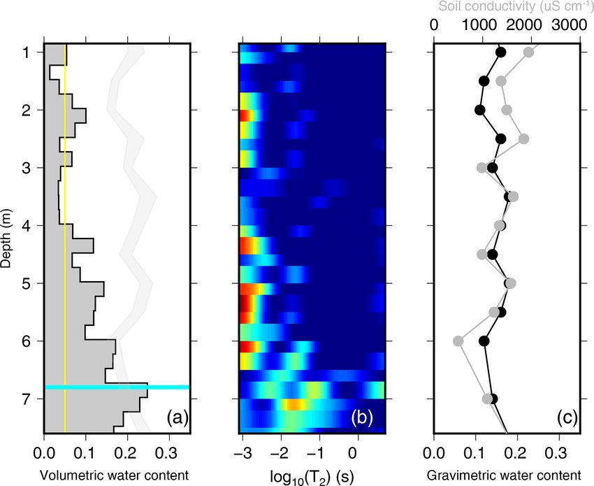
4358 B. A. Flinchum et al.: Identifying recharge under subtle ephemeral features in flat-lying semi-arid region
structure and the size of the transmitting loop and the ampli-
tude of the transmitted signal. For a more thorough descrip-
tion of the TEM technique, see Telford et al. (1990), Paras-
nis (1986), or Reynolds (2011).
We collected the TEM data using a Zonge Engineer-
ing NanoTEM system. The NanoTEM is a low-power,
fast-sampling TEM system that was specifically designed
to provide high-resolution images of the near surface (∼
50 m depth). The NanoTEM data were collected using
a 20 m × 20 m square transmitter loop with a 5 m × 5 m,
single-turn receiving loop. The transmitter coil had an out-
put current of 2 A and a turnoff of ∼ 2 µs. The receiving loop
sampled at 625 kHz, stacking 256 cycles at a repetition rate
of 32 Hz. The stacks were averaged and then inspected to re-
move noisy data in the late times. The NanoTEM data were
inverted using the Aarhusinv program, run using “smooth
model” settings (Auken et al., 2006, 2015). The 1D inver-
sion assumes laterally homogeneous layers. All NanoTEM
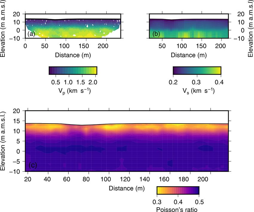
Figure 2. (a) The P-wave velocity results shown at 2× vertical ex-
soundings were inverted separately (i.e. there were no lateral aggeration. Areas where no rays pass through a model cell have
constraints) and placed next to one another and interpolated been masked out. (b) The S-wave velocity results shown at 2× ver-
to generate pseudo 2D profiles of bulk electrical conductivity. tical exaggeration. This image shows the 42 1D inversions side by
The quality of the inversion is determined by a misfit value side; no interpolation has been applied. (c) Profile of Poisson’s ratio
between the observed and modelled voltages. calculated using Eq. (1) and the profiles shown in (a) and (b).
3.7 Drill hole soil sample measurements
4 Results
Soil samples were collected at 0.25 m intervals from the con-
tinuous core that was retrieved during the shallow drilling 4.1 Seismic results
programme. Each soil sample was placed into an airtight
plastic container to prevent moisture loss and preserved for We use the P-wave profile generated by travel-time tomog-
later analysis in the laboratory for gravimetric water contents raphy (Fig. 2a) and the S-wave profile estimated through
and soil pore water salinity. The gravimetric water content the inversion of surface waves (Fig. 2b) to create a Pois-
was determined as the water loss between the wet and dry son’s ratio profile (Eq. 1) (Fig. 2c). Under the assumption
sample after 3 d in an oven at 40◦ , using standard methodolo- that changes in Poison’s ratio are due to saturation and not
gies as described in Rayment and Higginson (1992). Salinity changes in lithology, Poisson’s ratio should increase to val-
(i.e. electrical conductivity) of the pore water was measured ues close to 0.5 as saturation approaches 100 %. In our data,
using a 1 : 5 mass ratio by combining 20 g of soil and 100 g Poisson’s ratio increases with depth and averages out to a
of ultra-pure water (He et al., 2012, p. 5; Rayment and Hig- value of ∼ 0.46 below an elevation of 5 m a.m.s.l. (Fig. 2c).
ginson, 1992). The samples were agitated by rotating in a An anomaly occurs between 60 to 80 m along the profile and
tumbler device for 48 h and left to settle for 1 h, and then an is the only location where high Poisson’s ratios (> 0.4) reach
electrical conductivity probe was used to measure the elec- the surface. This observation is not surprising given that this
trical conductivity of the supernatant. The soil water conduc- profile is driven by P-wave and S-wave profiles where at 60–
tivity was determined using the 1 : 5 ratio dilution factor. For 80 m along the profile we observed a drop in S-wave veloc-
the shallow drill hole, we have gravimetric water content and ities, while the P-wave velocities increased slightly (Fig. 2a
soil conductivity as a function of depth. To make compar- and b). Because the difference in P-wave and S-wave veloc-
isons with the NMR data, the gravimetric water content was ity is larger, Poisson’s ratio is also larger (Eq. 1).
converted into volumetric water content by multiplying an The P-wave velocity profile is characterized by two fea-
assumed soil density between 1.3 and 1.5 g cm−3 . We also tures. The first feature is a laterally homogeneous layer de-
assumed the density of water equal to 1 g cm−3 . fined by a consistent increase in velocity from about 0.3 to
1.5 km s−1 . The bottom of the feature is defined by a velocity
of ∼ 1.5 km s−1 and corresponds to the depth where the ver-
tical velocity gradient weakens significantly (Fig. S3d). This
boundary, which is clearly identified in the travel-time picks
(Fig. S2), defines the bottom of an approximately 13 m thick
horizontal layer at around 0 m elevation (Fig. 2a). The second
Hydrol. Earth Syst. Sci., 24, 4353–4368, 2020 https://doi.org/10.5194/hess-24-4353-2020B. A. Flinchum et al.: Identifying recharge under subtle ephemeral features in flat-lying semi-arid region 4359
feature is more subtle and is associated with a change in slope
in the travel-time picks between 60 and 80 m (Fig. S2a).
Because of the high quality of the seismic data, the inver-
sion was able to adjust this change in slope in the travel-
time curves (Fig. S2), which is reflected in the final model
(Fig. 2a).
Like the P-wave velocity profile, the S-wave profile is lat-
erally continuous (Fig. 2b). On average the S-wave velocity
increases from 0.2 km s−1 at the surface to 0.4 km s−1 in the
deepest parts of the model. There is an abrupt increase in
velocity around 0 m elevation (Fig. 2b), which is consistent
with the large change in velocity observed in the P-wave ve-
locity profile (Fig. 2a). There is one notable difference be-
tween the two profiles occurring between 60 and 80 m, ap-
proximately at the same location where we observed the sub-
tle increase in P-wave velocities; unlike the P-wave veloci-
ties, the S-wave velocities are defined by a slight decrease
in velocity (Fig. 2b), which was also a clear and observable Figure 3. Electrical conductivity results produced by the NanoTEM
feature in the picked dispersion curves (Fig. S4). soundings. The x axis is distance from the first geophone (Fig. 1).
Both panels are shown at 2× vertical exaggeration. (a) One-
4.2 TEM results dimensional conductivity profiles plotted at their inverted resolu-
tions as well as their spatial locations. (b) The interpolated conduc-
tivity section. The black contour represents 200 mS m−1 . The small
The 26 NanoTEM soundings show consistency between the
grey plus symbols represent the data used for the interpolation.
soundings (Fig. 3a). To ease comparisons to both the S-wave
and P-wave profiles, the soundings were interpolated to a
2.5 m×0.5 m grid. In this grid the distance along the x axis is and the water contents also increase (Fig. 4b). This gradual
relative to the start of the seismic profile (Fig. 1). The interpo- increase in the T 2 decay times and water content is likely to
lation was done using an adjustable tension continuous cur- be the capillary fringe, where the remaining pore space fills
vature spline (Smith and Wessel, 1990). In the interpolated from smallest to largest pores. At depths below the measured
section (Fig. 3b), the most resistive feature (< 200 mS m−1 ) water level (6.8 m), the T2 distributions normalize and have a
occurs at the ground surface and extends to an elevation of value just over 0.01 s, which is consistent with clays.
10 m a.m.s.l. (above mean sea level) between 60 and 80 m The gravimetric water content measured from the drill
along the profile. The resistive feature is well constrained hole core samples had an average of 0.15 with a stan-
by individual soundings (Fig. 3a) and extends both laterally dard deviation of 0.02 and showed very little variation
and at depth on both sides of the depression between 10 and with depth (Fig. 4c). The soil pore water conductivity also
5 m a.m.s.l. and from 40 to 160 m along the profile (Fig. 3b). showed little variation with depth, having an average con-
ductivity of 1123 µS cm−1 with a standard deviation of
4.3 NMR and soil sample results 424 µS cm−1 (Fig. 4c). When converted to mS m−1 (112.3 ±
42.5 mS m−1 ) the soil conductivities are in within the range
The downhole NMR results show that the volumetric water of conductivities observed in the TEM profile. In contrast
contents of the soil profile vary between 0 and 0.25 m3 m−3 , to soil conductivities, the measured groundwater conduc-
with a gradual increase with depth (Fig. 4a). The maxi- tivity was 14 750 µS cm−1 (conductivity of sea water is ∼
mum water content of 0.25 m3 m−3 was measured between 50 000 µS cm−1 ). The TEM conductivity represents an av-
6.75 and 7 m depth, consistent with the measured water level erage between the soil conductivity and groundwater con-
depth (6.8 m) (Fig. 4a). The average amplitude of the noise ductivity, which is why we do not observe high conductivity
in the water contents determined by NMR is ∼ 0.05 m3 m−3 . values below the water table (Fig. 3). There is also notable
Therefore, inverted water contents of less than 0.05 m3 m−3 difference in the gravimetric water contents and NMR wa-
are less reliable. Signals from the soundings can be found in ter contents (Fig. 3). This difference could be attributed to
the Supplement (Fig. S6). Above the water table, the NMR the fact that the NMR cannot detect water in the smallest
data showed a rise in water contents above 0.05 m3 m−3 be- pores. Below the water table, where the assumption of fully
tween 1.75 and 3 m depth. The water within this region con- saturated pores is likely satisfied, the gravimetric water con-
tains low T2 relaxation times (< 0.01 s). A similar pattern in tents and NMR water contents are in much closer agreement
water content and T2 decay times occurs between 4 and 6 m (Fig. 4a).
depth (Fig. 4a and b). Around 6 m depth the T2 distributions
transition from shorter to longer (> 0.01 s) relaxation times
https://doi.org/10.5194/hess-24-4353-2020 Hydrol. Earth Syst. Sci., 24, 4353–4368, 20204360 B. A. Flinchum et al.: Identifying recharge under subtle ephemeral features in flat-lying semi-arid region
ferred water table depth. The value of 0.45 also validated
against the manual water level measurements (6.8 m depth
below ground) and the downhole NMR water content profile
from the drill hole (occurring at 220 m along the profile). It
also corresponds well with previous values given by Pasquet
et al. (2015a, b).
Under the assumption of a flat water table from the drill
hole, the contour value of 0.46 matches qualitatively the
depth to water between 0 and 60 m and again between 80 and
220 m (Fig. 5a). There is one notable deviation occurring
between 60 and 80 m where we highlight anomalies in all
three geophysical methods. We observed a slight increase
in P-wave velocities (Fig. 2a), slightly lower S-wave veloc-
ities (Fig. 2b), and a resistive feature in the NanoTEM data
(Fig. 3). As a result, the geophysically inferred water table
depth at this location along the profile differs from the man-
ually measured water level (Fig. 5a). We interpret this rise in
Figure 4. Results from the downhole NMR sounding and soil sam- Poisson’s ratios as the water table rising toward the surface
ples at the drill hole location versus depth (metres below ground beneath the subtle topographic depression in the landscape,
level; Fig. 1). (a) The water content profile from the downhole NMR representing the ephemeral drainage feature (Fig. 5b).
data. The thin vertical yellow line shows the average noise level Using a contour value of 0.46 provides an estimate for
(0.05 m3 m−3 ) below which water content estimates are question- the water table, but the boundary is fuzzy and possibly tran-
able. The thick horizontal cyan line represents the manually mea- sitional (Fig. 5a). The fuzziness of the boundary could be
sured water level from ground surface (6.8 m). The thin transparent
explained by two processes. First, partial saturation could
region is the volumetric water content estimated from the measured
gravimetric water content, assuming a soil density between 1.3 and
be occurring above the water table. Second, the water ta-
1.5 g cm3 . (b) The T2 distributions that produced the water content ble boundary could be well defined, but it is smoothed over
curves in (a). The maximum water contents are calculated by sum- by the geophysical inversions. The smoothing is difficult to
ming the area under the distribution. (c) Soil conductivity (grey) and quantify and is complicated by the fact that the P-wave and
gravimetric water contents (black) as a function of depth. S-wave velocities come from two different inversions based
on different physics. More research is needed to understand
and compare the sample volumes of the travel-time tomog-
5 Discussion raphy and surface wave inversions. The first interpretation of
a transitional zone between unsaturated and saturated sed-
5.1 Geophysically inferred water table depth iments is more likely because of observations in the NMR
data (Fig. 4) and the presence of water measured in the col-
To estimate a value of Poisson’s ratio that represents the wa- lected soil samples (Fig. 5c).
ter table, we laterally averaged two regions along the pro- In the downhole NMR data, we are confident with mea-
file to produce two 1D profiles with standard deviations. The sured water contents greater than 0.05 m3 m−3 . At 4 m depth
standard deviations represent the lateral variability. The first the water content is well above 0.05 m3 m−3 and shows a
laterally averaged region was between 60 and 80 m, where linear increase until a maximum value of 0.25 m3 m−3 is
the large anomaly occurs and where higher values of Pois- reached between 6.75 and 7.0 m below the surface (Fig. 4).
son’s ratio reach the surface (Fig. 5a). The second region Below the water table, the maximum water content likely
was chosen to be from 120 to 220 m because qualitatively represents total porosity. All the NMR responses above
it appears laterally uniform and includes the drill hole lo- the water table have low T2 decay times (Fig. 4b), which
cation (drill hole located at 220 m). These two averaged 1D can either be indicative of clay or caused by small pores,
profiles, when plotted side by side, show a similar trend in which preferentially fill and hold water after being drained
increasing Poisson’s ratio (Fig. 5c) but present a clear off- (i.e. leading to partial saturation of the medium) (Walsh et al.,
set. Near the surface the difference is largest, but the two 2014). The preferentially filled pores seems more likely be-
curves begin to converge near the water level measurement cause we know that the measurements were made within the
of 6.8 m depth below ground and the highest water con- vadose zone, and the measured gravimetric water contents of
tents from the NMR (Fig. 5c). At the inferred water table, the drill hole core showed that samples retained some mois-
the values of Poisson’s ratio between 60–80 and 120–220 m ture. The most important observation provided by the NMR
are 0.454 ± 0.004 and 0.475 ± 0.002, respectively (Fig. 5b). data is that partially saturated sediments exist at least 3 m
Here we use a value of 0.46 as the contour that represents above the water table (Fig. 5c). This partially saturated re-
the water table, which we refer to as the geophysically in- gion of the soil profile will likely increase Poisson’s ratios
Hydrol. Earth Syst. Sci., 24, 4353–4368, 2020 https://doi.org/10.5194/hess-24-4353-2020B. A. Flinchum et al.: Identifying recharge under subtle ephemeral features in flat-lying semi-arid region 4361 Figure 5. (a) Profile of Poisson’s ratio calculated using Eq. (1) and the profiles shown in Figs. 2 and 3. The solid black contour represents a Poisson’s ratio of 0.46. The dashed cyan line is the depth of water measured at the drill hole located at 220 m (6.8 m b.g.s. – below ground surface) and extends horizontally across the profile to be able to visualize the changes beneath the ephemeral feature. The dotted contour line is the 0.4 contour line, which is consistent with a 3 m thick partially saturated region. (b) Geophysically interpreted hydrogeological cross section. The unsaturated zone is quantified by areas with Poisson’s ratios less than 0.40. The partially saturated region, with a thickness of approximately 3 m (determined from NMR in c), has Poisson’s ratios between 0.4 and 0.46. The fully saturated region has Poisson’s ratios greater than 0.46. The geophysically inferred water table is approximated by the 0.46 contour in (a). (c) The water content profile from Fig. 4. The partially saturated region from 4 to 6.8 m depth is highlighted. The horizontal cyan bar is the manual water level measurement (6.8 m). Overlain on the water content profile are the two horizontally averaged 1D Poisson’s ratio profiles. The red line is averaged from 120 to 220 m and the maroon line is averaged between 60 and 80 m along the profile. Black dashed lines and solid crosses highlight the Poisson’s ratio contour values of 0.4 and 0.46 chosen in (a). Figure 6. The final hydrogeological framework for a subtle ephemeral surface water feature in the semi-arid landscape of the Northern Adelaide Plains. The underlying map is based on the seismic data. The yellow region is our interpreted region of fresher water that has recharged the shallow unconfined aquifer system. Here water flows across the land surface and collects into the subtle ephemeral drainage feature. From there water is recharged into the underlying aquifer system and the hydraulic gradient drives recharging water away from the groundwater mound, to either side. During the recharge process, the fresher recharge water is mixing with the ambient saline groundwater of the shallow Quaternary aquifer. and provides an explanation for the transitional and fuzzy pretation of seismic data, manual water level measurement, boundary we observe in the seismic data. Furthermore, if the and NMR data, we are therefore able to identify a mound in 0.46 contour is shifted upward 3 m based on the NMR ob- the water table underneath the small topographic depression, servation, it qualitatively matches the point where Poisson’s existing between 60 and 80 m along the profile (Fig. 5b). ratio begins to increase (Fig. 5a). From the combined inter- The NMR data and Poisson’s ratio suggest the existence of a https://doi.org/10.5194/hess-24-4353-2020 Hydrol. Earth Syst. Sci., 24, 4353–4368, 2020
4362           B. A. Flinchum et al.: Identifying recharge under subtle ephemeral features in flat-lying semi-arid region

∼ 3 m thick section of partially saturated sediments on top of    modelling exercise using Archie’s Law shows that if we re-
the water table along the profile (Fig. 5b).                      place the water in the pores with a more resistive fluid, it is
                                                                  possible to get a drop in electrical conductivity even if the
5.2    Geophysically identified recharge processes                saturation is increased (refer to Supplement). Thus the de-
                                                                  crease in electrical conductivity supports the interpretation
In the previous section we relied heavily on the seismic data,    that the rise in Poisson’s ratios is caused by an increase in
NMR data, soil cores, and water level to define a geophys-        water content and not an increase in clay content.
ically inferred water table depth along the study transect
(Fig. 5b). We argued for the existence of a 3 m thick par-        5.3   Hydrogeological implications
tially saturated region above the water table based on wa-
ter contents from the NMR data (Figure 5c). In this section       We combine all the geophysical observations to construct a
we utilize the bulk electrical conductivities obtained from the   hydrogeological interpretation of the study site (Fig. 6). First,
NanoTEM data to strengthen the interpretation that the Pois-      based on the seismic data and the measured water depth from
son’s ratio anomaly between 60 to 80 m along the transect         the nearby drill hole we can identify a rise in the water ta-
is caused by an increase in saturation to demonstrate that        ble beneath the small topographic depression. It is likely that
the subtle topographic surface depression acts as a localized     this rise in water table has a partially saturated region that is
recharge zone.                                                    ∼ 3 m thick above it. Because of the observed drop in electri-
   Ambiguities exist in geophysical measurements because          cal conductivities, we interpret this feature as a saturation in-
they measure physical properties that are related to the pro-     crease and not a change due to an increase in clay content. We
cesses that we are trying to understand. Although we do not       interpret the drop in electrical conductivities as fresher water
expect any lithological variation based on the known soil         diluting and mixing with the ambient saline groundwater of
and geological mapping of the area, it is possible that the       the Quaternary aquifer. The resistive feature lies above the
region of high Poisson’s ratios is a result of higher clay con-   partially saturated or saturated zones between 80 and 100 m
tent, since materials that are deformed easily will have higher   and again between 120 and 140 m (Fig. 6).
Poisson’s ratios. Poisson’s ratio for pure quartz, a stiff min-      Our study has shown that the smaller tributaries and
eral, is between 0.06 and 0.08, Kaolinite is 0.14, and clays      ephemeral streams across the lower-lying areas of the NAP
are around 0.34 and 0.35 (Mavko et al., 2009). It would be        are acting as localized sources for recharge to the Quaternary
reasonable to assume higher clay content as an alternative in-    and Tertiary aquifers. This suggests that there is localized ar-
terpretation to explain the higher Poisson’s ratios under the     eas of recharge across the NAP associated with these types
topographic surface depression. Here the conductivities from      of subtle features – an interpretation that is consistent with
the NanoTEM provide evidence to suggest that an increase in       the findings of Bresciani et al. (2018), which showed that the
clay content is unlikely. If the high Poisson’s ratio were due    main recharge mechanisms to the Quaternary and Tertiary
to an increased clay content, we would expect the electri-        aquifer systems across the NAP was through surface water
cal conductivities to rise – but we observe the opposite. The     infiltration along the large river systems (e.g. the Gawler and
subsurface is more resistive at the location where Poisson’s      Little Para rivers) that have their headwaters in the Mount
ratios rise.                                                      Lofty Ranges and outlets towards the coast.
   Underneath the small depression in topography between             It should be noted that our hydrogeological interpretation
60 and 80 m along the seismic profile we have anomalies           is based on a single snapshot in time. Without time-lapse
in all three geophysical data sets: (1) the P-wave veloci-        geophysical measurements, groundwater samples taken from
ties increase, (2) the S-wave velocities decrease, and (3) the    within the groundwater mound and either side, or long-term
electrical conductivities decrease. As discussed in the pre-      monitoring of groundwater observation wells, it is not pos-
vious section, the first two anomalies cause Poisson’s ra-        sible to definitively quantify the recharge rates in these sys-
tio to rise, which we interpret as a rise in the water ta-        tems. Nor is it possible to determine whether the groundwa-
ble or at a minimum increase in water saturation. Here we         ter mound is a result of a recent rainfall event or whether it
believe the decrease in electrical conductivity is the result     is a more stable feature. It seems reasonable, given the ev-
of more conductive groundwater being replaced by fresher          idence of ephemeral surface drainage features in the lidar
water that has infiltrated from rainfall events. Although we      data (Fig. 1) and the high clay content of the near subsurface
did not measure the electrical conductivity of rainwater, we      that surface water would flow towards subtle depressions in
know that the groundwater from the shallow aquifer at the         the landscape and eventually out to St Vincent Gulf (Fig. 6).
study site has a much higher conductivity (14 750 µS cm−1 )       These small ephemeral features are unmonitored, so it is un-
which is similar to observed salinities in the shallow Quater-    known how quickly or how much water flows through them
nary system across the NAP, which range between 2000 and          during storm events. The NAP are topographically flat so it is
13 000 mg L−1 (3075 to 20 000 µS cm−1 ) (Department for           possible that instead of surface water flowing out towards the
Water, 2010). Typically, an increase in saturation causes an      ocean, water might accumulate in these low-lying features af-
increase in electrical conductivity. A simplified and general     ter large rainfall or storm events and gradually infiltrate over

Hydrol. Earth Syst. Sci., 24, 4353–4368, 2020                                      https://doi.org/10.5194/hess-24-4353-2020
B. A. Flinchum et al.: Identifying recharge under subtle ephemeral features in flat-lying semi-arid region 4363
longer periods of time. The ponded water from such rainfall The NAP provided ideal conditions for us to exploit Pois-
events would produce localized recharge to the underlying son’s ratio to map the water table in detail. The NAP were
aquifer system (Fig. 6). The recharge water would be fresher ideal because the subsurface was broadly homogeneous, and
than the groundwater already in the Quaternary aquifer sys- there were no abrupt or lateral variations in the lithology.
tem. Lithological variation would complicate the interpretation
The hydrological conceptualization based on the geophys- of Poisson’s ratio because all the changes could not be at-
ical data (Fig. 6) could be confirmed or rejected by drilling tributed solely to changes in saturation. We were also specific
and sampling the groundwater via an additional shallow drill in selecting a location where the water table was between
hole across the shallow topographic depression. The com- 3 and 10 m depth. In order to image the saturated zone with
bination of geophysical data has provided a new perspec- seismic methodologies, we required an elastic contrast be-
tive that allows us to speculate about important local hy- tween the unsaturated and saturated zones. Although uncer-
drological processes taking place in the NAP. Furthermore, tainty is difficult to quantify given the different sample vol-
the combined geophysical approach presented here can be umes and wavelengths of the seismic wave field and Rayleigh
used to guide and plan more widespread investigations fo- waves (work that extends beyond the scope of this paper), we
cused on understanding the role of these subtle ephemeral believe that having at least 3 m of unsaturated zone above the
features across this flat semi-arid landscape. The combined water table should provide a strong enough contrast to image.
geophysical approach provided a vital conceptual framework Furthermore, the inversion of surface waves is limited by the
for the hydrological processes occurring within the area. Fu- frequency content of the source and the peak geophone fre-
ture work should focus on combining the geophysical mea- quency. In our case, with 14 Hz geophones, imaging a water
surements with more traditional hydrological and geochemi- table that is below ∼ 10–12 m would be difficult. Thus, to im-
cal measurements to fully explore and test the hydrogeolog- prove chances of success, the seismic approach should be ap-
ical conceptualization suggested in this paper and the tran- plied in regions where the water table is between 3 and 10 m
sient nature of the recharge mechanisms (Fig. 6). in a homogeneous material. We used the existing 47 bore-
holes from another study (Hatch et al., 2019) to select a site
that satisfied this condition.
5.4 Applying the combined geophysical approach to
The additional information provided by the NanoTEM
other semi-arid regions
data helped reduce ambiguities observed in the Poisson’s ra-
tio profile. Without this additional information it would have
Throughout this study we used well-established geophysical been difficult to determine whether the anomaly was caused
methods. Each of these methods have open-source inversions by an increased clay content or an increase in water con-
available or the equipment comes with easy-to-use inversion tent. Thus, the electrical conductivity data were critical to our
software. Thus, there is nothing novel about the processing hydrological interpretation. It should be noted that the Nan-
of each individual geophysical data set, but the combination oTEM data could also be replaced by another independent
of all these methods can be used to rapidly explore flat-lying observation, e.g. other near-surface geophysical methods or
features to test a given conceptual model of the recharge pro- soil conductivity profiles at several locations along the tran-
cesses in a flat-lying semi-arid landscape. In order to facil- sect. Regardless, more observational evidence, even if they
itate and expand the use of this combined geophysical ap- are point measurements, will aid in the interpretation of the
proach to other semi-arid streams or features, we highlight geophysical images.
some of the uncertainty, limitations, advantages, and critical
assumptions that went into building the hydrological concep-
tualization so that this methodology might be transferred to 6 Conclusions
other semi-arid areas that are common around the world.
We relied heavily on the manual water level measurement We have shown that the combination of P-wave and S-wave
and downhole NMR data. The geophysical mapped water ta- velocities, electrical conductivities, and surface NMR can
ble essentially extended from the water level that we were identify small-scale ephemeral recharge features in a semi-
able to measure at the drill hole location. The drill hole data arid landscape without the use of time-lapse measurements.
were critical to calibrate the value of Poisson’s ratio that we The seismic data were used to calculate Poisson’s ratio and
used to represent the water table. The method would be much served as the foundation to geophysically infer the water ta-
more powerful if the drill hole was not required, but because ble depth. The NMR data showed a 3 m thick region of par-
this was the first survey of its kind in the region we needed tially saturated sediments, and the electrical conductivities
to confirm where the water level was to interpret Poisson’s from the NanoTEM provided additional evidence to support
ratio. Now, with a value of 0.45 it would be possible to run a an increase in water content opposed to an increase in clay
survey without the drill hole and predict the water level with- content. The combination of all four data sets has provided a
out a drill hole. Thus, some validation is required prior to hydrogeological framework where we are observing fresher
extending the methodologies throughout the NAP. water recharging and replenishing the underlying saline Qua-
https://doi.org/10.5194/hess-24-4353-2020 Hydrol. Earth Syst. Sci., 24, 4353–4368, 2020You can also read