Uncertainty of simulated groundwater recharge at different global warming levels: a global-scale multi-model ensemble study
←
→
Page content transcription
If your browser does not render page correctly, please read the page content below
Hydrol. Earth Syst. Sci., 25, 787–810, 2021
https://doi.org/10.5194/hess-25-787-2021
© Author(s) 2021. This work is distributed under
the Creative Commons Attribution 4.0 License.

Uncertainty of simulated groundwater recharge at different global
warming levels: a global-scale multi-model ensemble study
Robert Reinecke1,2 , Hannes Müller Schmied2,3 , Tim Trautmann2 , Lauren Seaby Andersen4 , Peter Burek5 ,
Martina Flörke6 , Simon N. Gosling7 , Manolis Grillakis8 , Naota Hanasaki9 , Aristeidis Koutroulis10 , Yadu Pokhrel11 ,
Wim Thiery12,13 , Yoshihide Wada5,14 , Satoh Yusuke5,9 , and Petra Döll2,3
1 International  Centre for Water Resources and Global Change (UNESCO), 56002 Koblenz, Germany
2 Institute of Physical Geography, Goethe University Frankfurt, 60438 Frankfurt, Germany
3 Senckenberg Leibniz Biodiversity and Climate Research Centre (SBiK-F) Frankfurt, 60325 Frankfurt, Germany
4 Potsdam Institute for Climate Impact Research, Telegrafenberg A31, 14473 Potsdam, Germany
5 International Institute for Applied Systems Analysis, Schlossplatz 1, 2361 Laxenburg, Austria
6 Institute of Engineering Hydrology and Water Resources Management, Ruhr-University Bochum, 44801 Bochum, Germany
7 School of Geography, University of Nottingham, Nottingham NG7 2RD, United Kingdom
8 Institute for Mediterranean Studies, Foundation for Research and Technology Hellas, Rethymno 74100, Greece
9 National Institute for Environmental Studies, Tsukuba, Japan
10 School of Environmental Engineering, Technical University of Crete, Chania 73100, Greece
11 Department of Civil and Environmental Engineering, Michigan State University, East Lansing, Michigan 48824, USA
12 Department of Hydrology and Hydraulic Engineering, Vrije Universiteit Brussel, Pleinlaan 2, 1050 Brussels, Belgium
13 Institute for Atmospheric and Climate Science, ETH Zurich, Universitaetsstrasse 16, 8092 Zurich, Switzerland
14 Department of Physical Geography, Faculty of Geosciences, Utrecht University, Utrecht, the Netherlands

Correspondence: Robert Reinecke (robert.reinecke@uni-potsdam.de)

Received: 18 May 2020 – Discussion started: 8 June 2020
Revised: 15 January 2021 – Accepted: 19 January 2021 – Published: 19 February 2021

Abstract. Billions of people rely on groundwater as being an       the different GHM–GCM combinations, and statistically sig-
accessible source of drinking water and for irrigation, espe-      nificant changes are only computed for a few regions of
cially in times of drought. Its importance will likely increase    the world. Statistically significant GWR increases are pro-
with a changing climate. It is still unclear, however, how         jected for northern Europe and some parts of the Arctic, East
climate change will impact groundwater systems globally            Africa, and India. Statistically significant decreases are sim-
and, thus, the availability of this vital resource. Groundwa-      ulated in southern Chile, parts of Brazil, central USA, the
ter recharge is an important indicator for groundwater avail-      Mediterranean, and southeastern China. In some regions, re-
ability, but it is a water flux that is difficult to estimate as   versals of groundwater recharge trends can be observed with
uncertainties in the water balance accumulate, leading to pos-     global warming. Because most GHMs do not simulate the
sibly large errors in particular in dry regions. This study in-    impact of changing atmospheric CO2 and climate on vege-
vestigates uncertainties in groundwater recharge projections       tation and, thus, evapotranspiration, we investigate how esti-
using a multi-model ensemble of eight global hydrological          mated changes in GWR are affected by the inclusion of these
models (GHMs) that are driven by the bias-adjusted out-            processes. In some regions, inclusion leads to differences in
put of four global circulation models (GCMs). Pre-industrial       groundwater recharge changes of up to 100 mm per year.
and current groundwater recharge values are compared with          Most GHMs with active vegetation simulate less severe de-
recharge for different global warming (GW) levels as a re-         creases in groundwater recharge than GHMs without active
sult of three representative concentration pathways (RCPs).        vegetation and, in some regions, even increases instead of de-
Results suggest that projected changes strongly vary among         creases are simulated. However, in regions where GCMs pre-

Published by Copernicus Publications on behalf of the European Geosciences Union.
788                R. Reinecke et al.: Uncertainty of simulated groundwater recharge at different global warming levels

dict decreases in precipitation and where groundwater avail-       face water and groundwater and the impact of humans and
ability is the most important, model agreement among GHMs          the changing climate on the groundwater system (de Graaf
with active vegetation is the lowest. Overall, large uncertain-    et al., 2019; Reinecke et al., 2019). Neglecting capillary rise
ties in the model outcomes suggest that additional research        may lead to an overestimation of the decreases and increases
on simulating groundwater processes in GHMs is necessary.          in GWR due to a changing climate.
                                                                      Assessing the response of GWR to climate change is diffi-
                                                                   cult even at the local scale, with one of the reasons being that
                                                                   groundwater recharge, different from streamflow, is rarely
1   Introduction                                                   measured, and long time series of groundwater recharge are
                                                                   not available (Earman and Dettinger, 2011). In local ground-
The critical role of groundwater as an accessible source for       water modeling, groundwater recharge is often determined
irrigation and of drinking water, in particular during dry peri-   by calibration using hydraulic head observation, while in-
ods, droughts, and floods, will intensify with climate change      tegrated modeling relies on the partitioning of precipitation
because increased precipitation variability is expected to de-     into evapotranspiration, storage change, and runoff (GWR
crease the reliability of surface water supply (Taylor et al.,     plus surface and subsurface runoff). Moreover, projections
2013; Döll et al., 2018; Kundzewicz and Döll, 2009). While         of GWR often neglect the impact of changing climate and
demand for groundwater is likely to increase in the fu-            higher CO2 levels on plants and, thus, evapotranspiration and
ture, groundwater abstractions have already led to depleted        GWR (Taylor et al., 2013). With higher CO2 levels, terres-
aquifers in many regions around the globe (Thomas and              trial plants open their stomata less, which reduces evapotran-
Famiglietti, 2019; Cuthbert et al., 2019a; Wada et al., 2012;      spiration and increases runoff (physiological effect), while
Konikow and Kendy, 2005; Döll et al., 2014b). They have            they might grow better, increasing evapotranspiration (struc-
also resulted in the reduction in groundwater discharge to         tural effect; Gerten et al., 2014). Vegetation models that in-
rivers, with negative impacts on water availability for hu-        clude these effects disagree about the balance of both effects
mans and freshwater biota, in particular during low-flow pe-       (Gerten et al., 2014). However, based on a large ensemble
riods (Herbert and Döll, 2019). To what extent groundwater         of GCMs that include the impact of CO2 and changing cli-
can serve to sustain ecosystem health and to support human         mate on vegetation and evapotranspiration, rising CO2 can
adaptation to climate variability and change strongly depends      be expected to decrease transpiration and, thus, increase to-
on future groundwater availability, which is strongly affected     tal runoff (Milly and Dunne, 2016). Therefore, GHMs that
by climate change (Kundzewicz and Döll, 2009; Döll, 2009;          do not consider active vegetation may underestimate runoff,
Taylor et al., 2013; Cuthbert et al., 2019b).                      and, thus, GWR increases, or they may overestimate GWR
   Groundwater recharge (GWR) is a central indicator of po-        decreases.
tential groundwater availability (Herbert and Döll, 2019).            While there have been review articles on the relation be-
GWR is the vertical water flux to the groundwater from the         tween groundwater and climate change (Smerdon, 2017; Jing
soil (diffuse GWR) and from surface water bodies (point or         et al., 2020; Refsgaard et al., 2016), global-scale studies that
focused recharge; Small, 2005). It is a function of the lo-        quantify the impact of climate change on GWR are rare. They
cal climate, topography, soil, land cover, land use (urban-        have evolved regarding the way climate scenarios are imple-
ization, woodland establishment, crop rotation, and irriga-        mented and how many global climate models (GCMs) and
tion practices), atmospheric CO2 concentrations, and geol-         GHMs are included in the study. While Döll (2009) could
ogy (Small, 2005). Changes in GWR alter groundwater lev-           only use the delta change method to integrate information
els and their temporal patterns, which affect vital ecosystem      from two GCMs in the GHM WaterGAP (Alcamo et al.,
services (Kløve et al., 2014). Knowledge of the dynamics           2003; Müller Schmied et al., 2014), Portmann et al. (2013)
and process interactions determining GWR is a fundamen-            could feed their simulations of future changes in GWR with
tal prerequisite for assessing groundwater quality and quan-       WaterGAP directly by means of the bias-adjusted output
tity under climate change (Green et al., 2011). The simula-        with five GCMs. They found that changes in GWR increase
tion of GWR is possibly one of the most challenging compo-         with increasing greenhouse gas emissions. Acknowledging
nents of the water budget as it accumulates the uncertainties      that not only GCMs but also GHMs contribute to the uncer-
of all other components of the budget. Especially in semi-         tain translation of emissions scenarios to changes in GWR
arid regions, uncertainties in precipitation and evapotranspi-     (Moeck et al., 2016), the study of Döll et al. (2018) included
ration (Wartenburger et al., 2018) lead to considerable uncer-     two GHMs (WaterGAP and LPJmL – Lund Potsdam Jena
tainty in recharge. An additional factor in estimating ground-     managed Land; Rost et al., 2008; Schaphoff et al., 2013)
water recharge is the simulation of the groundwater table          driven by the bias-adjusted output of four GCMs. They eval-
and, thus, capillary rise and focused recharge. This has not       uated relative changes in GWR with climate change, which
been achieved yet in GHMs; however, recently, global hy-           can arguably serve as a better indicator of climate change
drological models (GHMs) started integrating gradient-based        hazard than absolute changes in GWR. On the other hand, the
groundwater models to better estimate the flows between sur-       usage of relative change led to the result that change in GWR

Hydrol. Earth Syst. Sci., 25, 787–810, 2021                                          https://doi.org/10.5194/hess-25-787-2021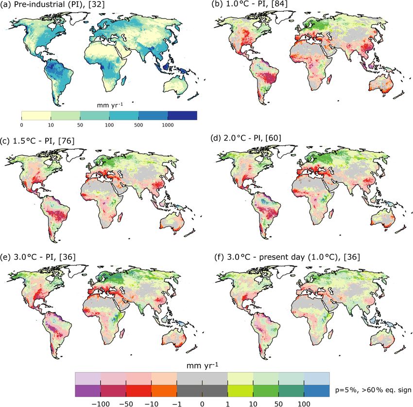
R. Reinecke et al.: Uncertainty of simulated groundwater recharge at different global warming levels                          789

could not be reliably computed for 55 % of the global land        2     Methods
area due to very small GWR for the reference period simu-
lated by LPJmL (Döll et al., 2018). While the LPJmL model         2.1     Simulation of groundwater recharge
considered, differently to the WaterGAP model, the effect of
rising CO2 on groundwater recharge, the impact of this on         This study encompasses eight GHMs that differ in their rep-
GWR projections were not analyzed in Döll et al. (2018). In       resentation of various hydrological processes. Four of these
general, studies investigating the difference between GHMs        models are able to simulate the impact of evolving CO2 con-
with and without dynamic vegetation are rare (Davie et al.,       centrations on vegetation: CLM 4.5, JULES-W1, LPJmL,
2013).                                                            and MATSIRO (Table 1). In the following, we use the term
   This study assesses the impact of climate change on GWR        active vegetation for models that consider the physiological
based on the output of a multi-model ensemble encompass-          effect of changes in CO2 on vegetation and the term dynamic
ing eight GHMs, each forced by the bias-adjusted output of        vegetation for the models that allow for changing vegeta-
four GCMs under three different representative concentra-         tion regarding leaf area index (LAI) and/or vegetation type.
tion pathways (RCPs). The ensemble was generated in the           A comprehensive overview of GHMs and their properties
framework of the Inter-Sectoral Impact Model Intercompar-         can be found in Sood and Smakhtin (2015). Detailed model
ison Project (ISIMIP) using simulation protocol ISIMIP2b          descriptions and evaluations of the models can be found in
(Frieler et al., 2017). The ISIMIP global water sector in-        the primary publications referred to in the subsections below
corporates global models, including water resources models,       and Telteu et al. (2021; for the model parameterization see
land surface models, and dynamic vegetation models, which         Sect. 2.2). The definition of GWR and groundwater varies in
can compute water flows and storages on the continents of         between GHMs (discussed in Sect. 4). The analysis in this
the Earth; in this study, all three model types are referred to   study is based on monthly GWR (variable qr in ISIMIP) in
as GHMs. The ISIMIP2b ensemble has already been used in           0.5◦ × 0.5◦ grid cells simulated by the eight GHMs taking
multiple climate change studies investigating, for example,       part in the ISIMIP2b protocol (Frieler et al., 2017). Some
flood risk (Willner et al., 2018; Thober et al., 2017; Alfieri    GHMs contained small negative GWR values, for example,
et al., 2017), low flows in Europe (Marx et al., 2018), evapo-    due to capillary rise; these values were set to zero in the anal-
transpiration (Wartenburger et al., 2018), runoff and snow in     ysis. We do not consider focused recharge in this study as
Europe (Donnelly et al., 2017), drought severity (Pokhrel et      no model has offered a reliable implementation of these pro-
al., 2021), heat uptake by inland waters (Vanderkelen et al.,     cesses until now. Also, none of the models simulate the depth
2020), and multi-sectoral impacts (Byers et al., 2018; Lange      of the groundwater table beneath the land surface, which
et al., 2020).                                                    does not allow us to correctly attribute delays in recharge due
   We analyze how GWR is projected to change globally and         to water table depth.
regionally for multiple global warming (GW) levels, deter-
mine the contributions from GHMs and GCMs to the vari-            2.1.1    WaterGAP2
ance of simulated changes, and discuss the implications for
future assessments of global groundwater resources. Further-      The WaterGAP2 model (Alcamo et al., 2003) computes hu-
more, we show the effect of including the physiological im-       man water use in five sectors and the resulting net abstrac-
pacts of evolving CO2 on global estimates of GWR. To this         tions from groundwater and surface water for all land areas
end, the remainder of this paper is structured as follows.        of the globe, excluding Antarctica. These net abstractions are
Section 2 provides an overview of the used GHMs and the           then taken from the respective water storages in the Water-
methods for calculating changes in GWR per GW level and           GAP Global Hydrology Model (WGHM; Müller Schmied
sources of uncertainty. The results in Sect. 3 show the signif-   et al., 2014; Döll et al., 2003, 2012, 2014b). With daily
icant changes in GWR per GW and the differences between           time steps, WGHM simulates flows among the water stor-
GHMs and GCMs. We then compare the influence of GCMs,             age compartments canopy, snow, soil, groundwater, lakes,
GHMs, and RCPs on the variance of simulated GWR, assess           human-made reservoirs, wetlands, and rivers. GWR in Wa-
the differences in GWR due to including dynamic vegetation        terGAP2 is calculated as being a fraction of runoff from land
in GHMs, and compare the GHM simulations to interpolated          based on soil texture, relief, aquifer type, and the existence
measured GWR. The paper closes with a discussion of these         of permafrost or glaciers, taking into account a soil-texture-
findings (Sect. 4) and conclusions (Sect. 5).                     dependent maximum daily groundwater recharge rate (Döll
                                                                  and Fiedler, 2008). If a grid cell is defined as semiarid or arid
                                                                  and has a medium or coarse soil texture, GWR will only oc-
                                                                  cur if daily precipitation exceeds a critical value (Döll and
                                                                  Fiedler, 2008); otherwise, the water runs off. Runoff from
                                                                  land that does not contribute to GWR is transferred to sur-
                                                                  face water bodies as fast surface runoff. WaterGAP further
                                                                  computes focused recharge beneath surface water bodies in

https://doi.org/10.5194/hess-25-787-2021                                          Hydrol. Earth Syst. Sci., 25, 787–810, 2021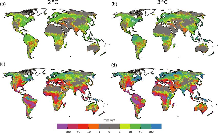
790                 R. Reinecke et al.: Uncertainty of simulated groundwater recharge at different global warming levels

Table 1. Overview of which models are able to simulate the impact of evolving CO2 concentrations on vegetation and how it is implemented.

        GHM                Considers    Summary of considered vegetation processes in ISIMIP2b                 Reference
                           CO2
        WaterGAP2          No           –                                                                      –
        CLM4.5             Yes          Photosynthesis depends on rootzone soil moisture availability.         Di Liu and Mishra
                                        The description is similar to LPJmL listed below. The area a           (2017)
                                        population of plant functional types (PFTs) takes up is prescribed
                                        and only changes if the input data changes.
        H08                No           –                                                                      –
        JULES-W1           Yes          Evapotranspiration is considered from five PFTs and four non-          Best et al. (2011),
                                        vegetative surface types. Each grid cell is composed of different      Clark et al. (2011)
                                        fractions of those nine surface types. Transpiration occurring from
                                        vegetation is based on the photosynthetic process, which is subject
                                        to stomatal conductance regulated by the CO2 concentration.
                                        Furthermore, transpiration is also controlled by soil moisture
                                        availability in the rootzone.
        LPJmL              Yes          Vegetation composition is determined by the fractional coverage of     Schaphoff et al.
                                        PFTs at the grid scale. PFTs are defined to account for the variety    (2018)
                                        in structure and function within a stand and are therefore simulated
                                        as average individuals competing for light and water according to
                                        their crown area, LAI, and rooting profiles. The vegetation
                                        dynamics component of LPJmL includes carbon allocation to
                                        different PFT tissue compartments, PFT interaction, and
                                        establishment and mortality processes. Photosynthesis and
                                        stomatal response are simulated following Farquhar et al. (1980)
                                        and the generalization by Collatz et al. (1991) for global
                                        modeling, based on the function of absorbed photosynthetically
                                        active radiation, temperature, day length, and canopy conductance
                                        for each PFT present in a grid cell.
        PCR-GLOBWB         No           –                                                                      –
        CWatM              No           –                                                                      –
        MATSIRO            Yes          The consideration of CO2 effects is functionally similar to that in    Takata et al. (2003)
                                        CLM, and there is no dynamic vegetation scheme. CO2 is
                                        prescribed in the model, which is used in the photosynthesis
                                        scheme to calculate stomatal conductance, among other
                                        parameters, following Farquhar et al. (1980). Soil moisture stress
                                        on photosynthesis is considered, using moisture availability in the
                                        rootzone with root the distribution fraction in each soil layer. All
                                        of that is done for different vegetation or plant functional types.

semiarid and arid grid cells, which is not considered in this           ence and are influenced by climate, including CO2 , across a
study.                                                                  variety of spatial and temporal scales (Lawrence et al. 2011).
                                                                        Individual land grid points can be composed of multiple land
2.1.2   CLM4.5                                                          units due to the nested tile approach, which enables the im-
                                                                        plementation of multiple soil columns and represents biomes
The Community Land Model version 4.5 (CLM4.5;                           as a combination of different plant functional types. Ground-
Lawrence et al., 2011; Oleson et al., 2013; Swenson and                 water processes, including sub-surface runoff, recharge, and
Lawrence, 2015) is the land component of the Community                  water table depth variations, are simulated based on the SIM-
Earth System Model (CESM), a fully coupled, state-of-the-               TOP scheme (SImple groundwater Model TOPgraphy based;
art Earth system model (Hurrell et al., 2013). CLM is a land            Niu et al., 2007; Oleson et al., 2013).
surface model representing the physical, chemical, and bio-
logical processes through which terrestrial ecosystems influ-

Hydrol. Earth Syst. Sci., 25, 787–810, 2021                                                 https://doi.org/10.5194/hess-25-787-2021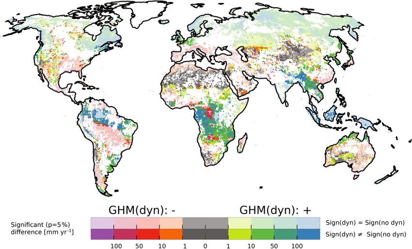
R. Reinecke et al.: Uncertainty of simulated groundwater recharge at different global warming levels                           791

2.1.3   H08                                                        the ISIMIP2b protocol, seepage from the base soil layer is re-
                                                                   ported as both GWR and groundwater runoff, which is routed
H08 (Hanasaki et al., 2018) is a GHM that includes various         directly (with no time delay) back into the river system.
components for water use and management. It consists of five
major components, namely a simple bucket-type land surface         2.1.6   PCR-GLOBWB
model, a river routing model, a crop growth model, which is
mainly used to estimate the timing of planting, harvesting,        PCR-GLOBWB (PCRaster Global Water Balance; Sutanud-
and irrigation in cropland, a reservoir operation model, and a     jaja et al., 2018); simulates the water storage in two vertically
water abstraction model. The abstraction model supplies wa-        stacked soil layers and an underlying groundwater layer. Wa-
ter to meet the daily water demand of three sectors (irrigation,   ter exchanges are simulated between the layers (infiltration,
industry, and municipality) from six available and accessi-        percolation, and capillary rise) and the interaction of the top
ble sources (river, local reservoir, aqueduct, seawater desali-    layer with the atmosphere (rainfall, evapotranspiration, and
nation, renewable groundwater, and non-renewable ground-           snowmelt). PCR-GLOBWB also calculates canopy intercep-
water) and one hypothetical one termed unspecified surface         tion and snow storage. Natural groundwater recharge is fed
water. It has two soil layers; one is to represent the unsatu-     by net precipitation, and additional recharge from irrigation
rated rootzone and the other the saturated zone (groundwa-         occurs as the net flux from the lowest soil layer to the ground-
ter). The scheme of GWR computation is identical to Döll           water layer, i.e., deep percolation minus capillary rise. The
and Fiedler (2008).                                                ARNO (a semi-distributed conceptual rainfall–runoff model;
                                                                   Todini, 1996) scheme is used to separate direct runoff, in-
2.1.4   JULES-W1                                                   terflow, and GWR. Groundwater recharge can be balanced
                                                                   by capillary rise if the top of the groundwater level is within
The Joint UK Land Environment Simulator (JULES; Best               5 m of the topographical surface (calculated as the height of
et al., 2011; W1 stands for water-related simulations in the       the groundwater storage over the storage coefficient on top
ISIMIP framework) is a land surface model initially devel-         of the streambed elevation and the sub-grid distribution of
oped by the Met Office as the land surface component of the        elevation).
Met Office Unified Model. JULES is a process-based model
                                                                   2.1.7   CWatM
that simulates the carbon, water, energy, and momentum
fluxes between land and atmosphere, including plant–carbon         The Community Water Model (CWatM) is a large-scale inte-
interactions (Clark et al., 2011). The rainfall that reaches the   grated hydrological model which encompasses general sur-
ground is partitioned into Hortonian surface runoff and an         face and groundwater hydrological processes, including hu-
infiltration component. A total of four soil layers represent      man hydrological activities such as water use and reservoir
the soil column, with a total thickness of 3 m, with a unit        regulation (Burek et al., 2020). CWatM takes six land cover
hydraulic head gradient lower boundary condition and no            classes into account and applies the tile approach. This hy-
groundwater component. The water that infiltrates the soil         drological model has three soil layers and one groundwater
moves down the soil layers that are updated using a finite         storage. The depth of the first soil layer is 5 cm, and the depth
difference form of the Richards equation (Best et al., 2011).      of second and third layers vary over grids, depending on the
The saturation excess water from the bottom soil layer be-         rootzone depth of each land cover class, resulting in total soil
comes subsurface runoff that can be considered to be GWR           depth of up to 1.5 m. Groundwater storage is designed be-
(Le Vine et al., 2016).                                            ing as a linear reservoir. CWatM includes preferential bypass
                                                                   flow directly into groundwater storage and capillary rise from
2.1.5   LPJmL                                                      groundwater storage and percolation from the third soil layer
                                                                   to groundwater storage. Hence, the groundwater recharge re-
Lund Potsdam Jena managed Land (LPJmL) is a dynamic                ported by CWatM in ISIMIP2b is the net recharge calculated
global vegetation model that simulates the growth and pro-         from these three terms.
ductivity of both natural and agricultural vegetation as be-
ing coherently linked through their water, carbon, and en-         2.1.8   MATSIRO
ergy fluxes (Schaphoff et al., 2018). The soil column is di-
vided into six active hydrological layers, with a total thick-     The Minimal Advanced Treatments of Surface Interaction
ness of 13 m depth. Percolation of infiltrated water through       and RunOff (MATSIRO; Takata et al., 2003) is a global
the soil column is calculated according to a storage routine       land surface model initially developed for an atmospheric–
technique that simulates free water in the soil bucket (Arnold     ocean general circulation model, the Model For Interdisci-
et al., 1990). Excess water over the saturation levels pro-        plinary Research On Climate (Hasumi and Emori, 2020).
duces lateral runoff in each layer (subsurface runoff). GWR        This process-based model calculates water and energy flux
is considered to be percolation (seepage) from the bottom          and storage at and below the land surface, also consider-
soil layer. As there is no groundwater storage in LPJmL, for       ing the stomatal response to CO2 increase in the photosyn-

https://doi.org/10.5194/hess-25-787-2021                                           Hydrol. Earth Syst. Sci., 25, 787–810, 2021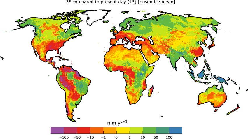
792                 R. Reinecke et al.: Uncertainty of simulated groundwater recharge at different global warming levels

thesis process. The offline version of MATSIRO used for             2.3   Determining stabilized warming levels
the ISIMIP2b simulation explicitly takes vertical ground-
water dynamics into account, including groundwater pump-            In order to derive policy-relevant information, we assessed
ing (Pokhrel et al., 2012, 2015). Soil moisture flux between        impacts framed in terms of GW levels (1, 1.5, 2, and 3◦ C)
the 15 soil layers is expressed as a function of the verti-         with respect to the GW of 0◦ C in PI conditions (James et
cal gradient of the hydraulic potential, which is the sum           al., 2017). The time of passing a warming level is defined
of the matric potential and the gravitational head, and the         as the first time the 31-year running mean of the global aver-
soil moisture movement is calculated by Richards equation.          aged annual mean temperature reaches above that level. Each
MATSIRO calculates net groundwater recharge as a bud-               GCM reaches different GW at different times (Table 2), de-
get of gravitational drainage into and capillary rise from the      pending on the RCPs (van Vuuren et al., 2014). For each
layer where the groundwater table exists. A simplified TOP-         GW level (1, 1.5, 2, and 3◦ C), time slice of 31 years (i.e.,
MODEL (TOPography-based MODEL; Beven and Kirkby,                    15 before the level was reached, and 15 after) for each GCM
1979; Stieglitz et al., 1997) is used to represent surface runoff   and for each RCP, in which that GW is reached, are used.
processes, and groundwater discharge is simulated by using          Using this time slice, a yearly mean GWR at 0.5◦ spatial res-
an unconfined aquifer model (Koirala et al., 2014).                 olution was calculated for the GHMs that were forced with
                                                                    the particular combination of GCM and RCP (Fig. 1). Addi-
2.2   Model simulations                                             tionally, a PI reference was calculated for each GCM, RCP,
                                                                    and GHM combination for the same time slice in which the
Each GHM is forced by bias-adjusted data from the fol-              GW level was reached in a particular RCP–GCM combina-
lowing four GCMs: GFDL-ESM2M, HadGEM2-ES, IPSL-                     tion using the PI reference simulation (see Sect. 2.2). Fig-
CM5A-LR, and MIROC5. Further details on the selection of            ure 1 illustrates the methodology by showing two unspecified
climate models and the bias correction can be found in Frieler      RCPs and the PI comparison paths.
et al. (2017), Lange (2018, 2019), Hempel et al. (2013), and           Considering that not all RCP/GCM combinations reach
online at ISIMIP (2018). The bias adjustment method used            higher warming levels (Table 2), not all ensembles have the
for the GCMs in ISIMIP2b is using a trend-preserving al-            same size. Theoretically, the maximum ensemble size is 96,
gorithm (Frieler et al., 2017) with the EWEMBI data set             with a combination of 8 GHMs, 4 GCMs, and 3 RCPs (2.6,
(Lange, 2018) as the baseline (reference) climate condition.        6.0, and 8.5). Because projections under RCP8.5 were not
The simulations in this study span the period from 1861             available for PCR-GLOBWB, the maximum ensemble size
to 2099. All GHMs (except for PCR-GLOBWB, which                     is 84. The smallest ensemble (for 3◦ C) consists of 36 mem-
misses the RCP8.5 run) simulate the RCPs 2.6, 6.0, and 8.5.         bers.
   The pre-industrial period (PI) is defined in ISIMIP
from 1661 to 1860, whereas the historical period is defined         2.4   Calculation of model variance
from 1861 to 2005. Additionally, for the RCP and histori-
cal simulations, ISIMIP defines PI simulations that repre-          To calculate whether the variance in absolute GWR change
sent an extended state of emissions scenarios from the PI           is mainly introduced through the GHMs or the GCMs, the
period until 2099 (and partially until 2300; not applicable         following equation was applied per model grid cell and
in this study). In this study, we always, unless stated other-      GW level.
wise, refer to PI by the simulation period of 1960–2099, with
the continued concentration levels of 1661–1860. Details on         Rvarmodel      2               2
                                                                         GWR = σGWR (GCMs)/ σGWR (GCMs)
the simulation setup can be found on the ISIMIP web page                          2

(ISIMIP, 2019) or in Frieler et al. (2017).                                   +σGWR  (GHMs) ,                             (1)
   Regarding the non-climatic drivers, all GHMs use, for
the time before 2006, so-called historical socioeconomic            where Rvarmodel
                                                                                GWR is the variance ratio of GCMs to GHMs,
                                                                     2
                                                                    σGWR  (GHMs) is the average variance of GWR change of all
pathway assumptions, e.g., historical water use, except for
                                                                    GHMs per GCM per RCP, and σGWR    2   (GCMs) is the average
CLM 4.5, which used the socioeconomic state of 2005. All
simulations for 2006–2099 are based on this assumed socio-          variance in GWR change of all GCMs per RCP per GHM.
economic state of 2005. For some models this affects the            The variance relative to the choice in RCP RvarRCP
                                                                                                                   GWR can be
abstraction from groundwater, which is not stimulated by            calculated similarly as follows:
all models (JULES-W1), or GWR directly due to irriga-
tion (H08, CLM, and PCR-GLOBWB). Details on the per-                RvarRCP
                                                                         GWR  =  σ 2
                                                                                  GWR  (RCPs)/      2
                                                                                                   σGWR (RCPs)
tinent scenario variables can be found in the ISIMIP protocol
                                                                                  2
(Frieler et al., 2017). Land use change was not considered.                   +σGWR   (GHMs) ,                              (2)

                                                                           2
                                                                    where σGWR (RCPs) is the average variance in GWR of all
                                                                    RCPs per GCM per GHM.

Hydrol. Earth Syst. Sci., 25, 787–810, 2021                                           https://doi.org/10.5194/hess-25-787-2021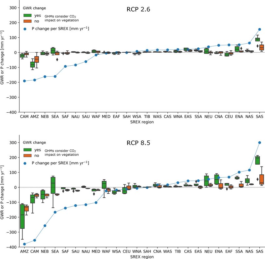
R. Reinecke et al.: Uncertainty of simulated groundwater recharge at different global warming levels                              793

Figure 1. Conceptual representation of how GW levels are determined for different GCMs, RCPs, and the PI comparison period.

Table 2. Overview of the warming levels and in which year they are reached in the corresponding GCM (ISIMIP, 2019).

                        Warming      RCP    GFDL-ESM2M         HadGEM2-ES       IPSL-CM5A-LR        MIROC5
                        level
                        1◦ C         2.6         2014              2012               1993            2015
                                     6.0         2016              2014               1993            2023
                                     8.5         2014              2012               1993            2014
                        1.5◦ C       2.6          –                2026               2009            2048
                                     6.0         2056              2032               2010            2052
                                     8.5         2036              2025               2009            2033
                        2◦ C         2.6          –                 –                 2029              –
                                     6.0         2076              2050               2029            2071
                                     8.5         2053              2037               2024            2048
                        3◦ C         2.6          –                 –                  –               —
                                     6.0          –                2076               2068             –
                                     8.5         2082              2056               2046            2071

2.5   Determining significant changes                                (i.e., a decrease or increase). In case of a low significance, all
                                                                     models may show large responses to climate change while
                                                                     their agreement on the amount or sign of change is low.
A model ensemble allows us to consider the uncertainty in
modeling physical processes as different models use differ-
ent algorithms and parameters for computing groundwater              3     Results
recharge. To determine whether changes in GWR due to
GW computed by the model ensemble are statistically sig-             3.1    Changes in groundwater recharge at different
nificant, we used the two-sample Kolmogorov–Smirnov (K–                     warming levels
S) test to compare the GWR values computed by all GHM–
GCM model combinations under, for example, PI conditions             To assess the impact of GW on GWR, Fig. 2 shows the en-
with the values at the various GW levels. The use of a two-          semble mean change of GWR between the current 1◦ C world
tailed t test is not advisable in this setting due to the small      and a potential 3◦ C GW. We chose to express changes as ab-
sample size (max. 84 in this study). Because the K–S test            solute change rather than relative change because zero, or
does not allow us to check whether the ensemble agrees on            close to zero, GWR in some regions of the world leads to
the sign of change in GWR, we applied an additional cri-             undefined or extremely large percentage increases and de-
terion to determine a significant change similar to Döll et          creases (Figs. S1 and S2 in the Supplement). The model
al. (2018). A change is only marked as statistically signifi-        mean shows large decreases of over 100 mm per year in
cant if the K–S test indicates a significant difference and at       South America and in the Mississippi Basin and decreases of
least 60 % of the model realizations of the ensemble (RCP,           up to 50 mm per year in the Mediterranean, East China, and
GCM, and GHM combinations) agree on the sign of change               West Africa. Increases of over 100 mm per year are promi-

https://doi.org/10.5194/hess-25-787-2021                                             Hydrol. Earth Syst. Sci., 25, 787–810, 2021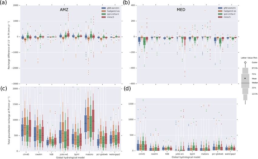
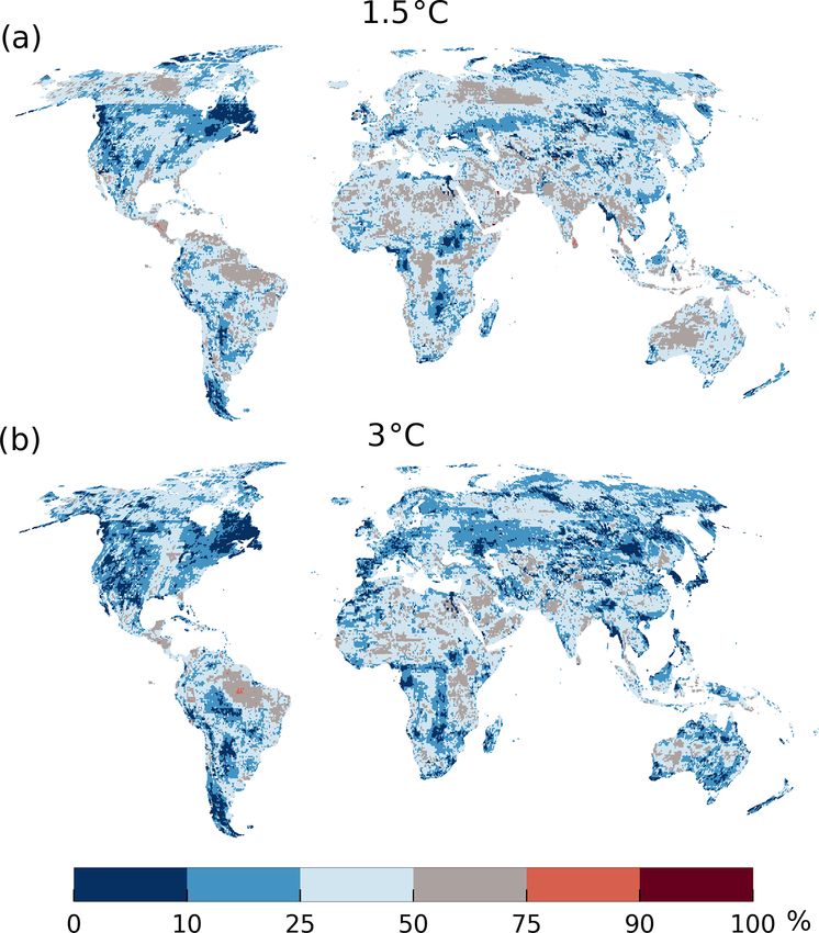
794                R. Reinecke et al.: Uncertainty of simulated groundwater recharge at different global warming levels

nent in Indonesia and East Africa. Individual GHM–GCM            change for this warming level. The global significant mean
model combinations compute much larger changes.                  change is −12 mm per year at 1.5◦ C GW.
   Ensemble mean changes, as shown in Fig. 2, may be low            At 2◦ C GW, increases in GWR over 100 mm per year are
in some areas, but this could be due to large positive changes   present in northern Java, the Amazon, and East Africa. De-
computed by some GHM–GCM model combinations being                creases are similar to 1.5◦ C GW, except for southern Chile
canceled by large negative changes by other model combi-         and the northern Andes, where decreases become more se-
nations. To assess the changes which show a high statistical     vere. However, on the significant global mean, these changes
agreement between the model combinations, we determine           balance out to −1 mm per year .
where computed changes of GWR are statistically significant         In a 3◦ C world, large areas of decreases in GWR of over
(Sect. 2.5). As a reference for the intensity of the changes,    100 mm per year in the Amazon Basin close to the Andes
Fig. 3a shows the mean GWR at PI averaged over all GHMs,         occur, and this is also the case in Guyana, Venezuela, West
RCPs, and GCMs from 1861 to 2099. The spatial pattern of         Africa, and the Mississippi Basin. Increases in GWR of over
GWR roughly agrees with the pattern of Mohan et al. (2018),      100 mm per year, in contrast, are visible in East Africa, India,
which is derived by inferring it from more than 700 small-       and northern Java. Increases of 50 to 100 mm per year domi-
scale GWR estimates. The global mean GWR for the PI pe-          nate in northern latitudes at 3◦ C warming compared to other
riod is 140 mm per year, which is very similar to the value of   GW levels. The global significant mean increases by +3 mm
134 mm per year determined by Mohan et al. (2018) for the        per year .
period 1981–2014 (see also Sect. 4).                                We have already reached a GW of approximately 1◦ C
   Figure 3b–e show the (statistical) significant (bright col-   (IPCC, 2018). Figure 3f shows the changes in GWR of a
ors; Sect. 2.5) mean absolute changes in GWR of the multi-       3◦ C GW compared to the present-day GW of already 1◦ C
model ensemble under a GW of 1.0, 1.5, 2.0, and 3.0◦ C           instead of the PI. Overall, the agreement among the mod-
compared to PI, i.e., GWR of the PI runs for the corre-          els is smaller than when the 3◦ C world is compared to PI.
sponding time slices (Sect. 2.3). For all GW levels com-         Only 8 % of the cells show significant changes. Decreases
pared to PI (Fig. 3b–e), consistent patterns of decreasing       over 100 mm per year are present in the Amazon Basin
GWR emerge for southern Chile, Brazil, central continen-         close to the Andes and on the coast of Guyana. Decreases
tal USA, the Mediterranean, and East China. Consistent and       of 50 to 100 mm per year are visible in Chile, the Missis-
significant increases can be observed for northern Europe        sippi Basin, the Caribbean, and southern France. Increases
and in general northern latitudes and East Africa. Signifi-      in GWR are again to be expected in the northern latitudes,
cant changes could only be derived for a small percentage of     southern Brazil, East Africa, and Southeast Asia, whereas the
the total grid cells. Only about 15 % of the cells, on average   latter shows increases over 100 mm per year for Malaysia.
for all GW levels, show significant increases or decreases.      The global significant mean change is +8 mm per year. Fig-
However, the patterns of non-significant (light colors) mean     ure S3 shows the mean and median changes of GWR per
changes are consistent with the significant changes and show,    latitude for all four GW levels, together with the standard de-
for example, larger areas of increases and decreases around      viation without a significance test. A decrease in mean GWR
the significant changes for the Amazon. The identification of    can be observed for all GW levels at 40◦ S, around 20◦ S
non-significance in most areas is due to the K–S test. The       (i.e., Namibia and Australia), and 5◦ N (Guyana). Increases
sign criterion affects mainly the Sahara and central Asia.       are visible at 60◦ N (northern Europe) and in the south, close
   At 1◦ C, GW (Fig. 3b) decreases of more than 100 mm per       to the Equator, presenting a large spread and sudden change
year are simulated in Southeast Asia, East China, Guyana,        in direction in the tropics. Increases at greater than 60◦ N are
and southern Brazil. Decreases between 100 and 50 mm per         likely due to a combination of different rain and snow pat-
year can be seen in central continental USA, southern Brazil,    terns and snowmelt timing.
southern Chile, the Mediterranean, central Africa, and East         Large areas of insignificant changes of GWR (light colors)
China. Increases in GWR of 50 and over 100 mm per year           in Fig. 3 can be traced back to the uncertainty in GWR in
are visible in the center of the Amazon, while decreases show    between GHMs and GCMs. Figure 4 shows absolute GWR
in the northeastern and southern part that increase with GW.     changes in a 1.5◦ C world compared to PI (Fig. 4a and b) and
Overall, the significant global change is −17 mm per year at     the absolute GWR at PI (Fig. 4c and d) for the SREX (Special
1◦ C.                                                            Report on Managing the Risks of Extreme Events and Dis-
   A 1.5◦ C GW shows only a limited increase in the Amazon       asters to Advance Climate Change Adaptation; Murray and
but similar increases in the rest of the world. Decreases in     Ebi, 2012; see Fig. S6 for a map of the SREX regions) region
GWR over 100 mm per year are now visible in Central Amer-        of the Amazon (left) and southern Europe/Mediterranean
ica, but decreases for Southeast Asia have vanished. Smaller     (right). Corresponding plots for all other SREX regions are
decreases, for example, in Australia, have also vanished in      provided in the Supplement. Similar to box plots, the letter-
a 1.5◦ C world. These effects are not necessarily due to no      value plots in Fig. 4 show the distribution of values among
changes in GWR but due to disagreements in the ensemble          the 0.5◦ grid cells belonging to the SREX region. Letter-
that do not allow us to determine a reliable and significant     value plots have the advantage of showing the distribution

Hydrol. Earth Syst. Sci., 25, 787–810, 2021                                        https://doi.org/10.5194/hess-25-787-2021
R. Reinecke et al.: Uncertainty of simulated groundwater recharge at different global warming levels                        795

Figure 2. Ensemble mean change in GWR (mm yr−1 ) between conditions of present-day warming of 1◦ C GW and at 3◦ C GW, averaged
over the GWR changes of all GHM–GCM model combinations.

of values outside of the usual interquartile range (IQR; Q25 –    altogether small GWR changes in all grid cells of the SREX
Q75 ). For example, for Fig. 4b CLM 4.5 with GFDL-ESM2-           regions. H08 and WaterGAP2, which apply similar ap-
ES, the mean change in GWR is −19 mm per year, the mid-           proaches to modeling GWR as a function of total runoff,
dle box represents the IQR showing that 50 % of changes are       show somewhat similar GWR changes.
close to zero or smaller than zero, the smaller box towards the      The four GHMs that take into account the impact of in-
negative changes shows that 12.5 % are smaller than −47 mm        creasing CO2 (Sect. 2.1) do not result in similar changes as
per year, whereas the additional missing box in the positive      compared to the other four models. It is to be expected from
direction hints that almost no values are larger than zero. The   the literature (Davie et al., 2013) that, with the physiolog-
horizontal size of the boxes is automatically scaled and does     ical effect, the decreases in GWR would be slighter in the
not carry any additional information.                             case of the CO2 -sensitive models, but that is not the case.
   Computed changes vary strongly among both GHMs and             This is likely due to the approach of analyzing GW lev-
GCMs (Fig. 4a and b). In the Amazon, JULES-W1 shows               els instead of RCPs and periods because different GCMs
a mean increase of 225 mm per year. Compared to Water-            reach a particular GW level at different times and CO2 levels.
GAP2, JULES-W1 estimates of GWR change are 147 mm                 This is further investigated in Sect. 3.3. On the global mean
per year higher for MIROC5 and 44 mm per year lower for           and for 1.5◦ C GW, LPJmL simulates the lowest PI GWR,
HadGEM. These differences are even large relative to the          whereas MATSIRO and CLM 4.5 produce the highest global
higher mean PI GWR in the Amazon compared to other re-            mean GWR (Fig. S4). PCR-GLOBWB simulates the largest
gions of the world (compare to MED in Fig. 4). Neverthe-          global mean decreases with HadGEM (Fig. S5). In contrast,
less, the PI estimates also differ by, for example, 122 mm        JULES-W1 and MATSIRO simulate increases of GWR on
per year between JULES-W1 and WaterGAP2 on the mean               the global mean for all GCMs except for HadGEM (Fig. S5).
for all GCMs and RCPs, and PI GWR is 625 mm per year                 To provide an overview of changes in GWR in each
smaller for H08 than for MATSIRO in the Amazon.                   SREX region, Table 3 shows the median, mean, and P25 and
   In the Mediterranean, almost all GHMs show the largest         P75 changes in GWR compared to PI for all regions (see
decreases in GWR with IPSL-CM5a-LR, followed by GFDL              Fig. S6 for a map of the SREX regions). Overall, north-
input, while HadGEM results in almost no change. However,         ern Europe shows the largest consistent increases in GWR,
the changes computed with each GCM input vary strongly            whereas the Amazon shows the largest consistent decreases,
among the GHMs. In general, CLM 4.5 and PCR-GLOBWB                except for 2◦ C, where southern Europe/Mediterranean shows
project the most considerable changes. The decrease in GWR        the largest decreases of 18.6 mm per year as the median. For
computed by CLM 4.5 with IPSL-CM5a-LR is 33 % of the              3◦ C, the Amazon shows the highest decreases in GWR with
mean GWR calculated for PI with that model combination.           −41.0 mm per year as median. Notably, Southeast Asia first
   Conversely, JULES-W1 simulates for most grid cells in          shows decreases of 13.1 mm per year with 1.0◦ C GW and
this SREX region the smallest PI GWR values (but also             then no change with 1.5 and 2◦ C and an increase in GWR
very high outliers) and, likely related, the smallest (mean)      of 13.5 mm per year with 3◦ C. Relative to PI, the changes
changes, together with MATSIRO and CWatM, which show              in the 3◦ C GW in the the Amazon only account for 10 % of

https://doi.org/10.5194/hess-25-787-2021                                         Hydrol. Earth Syst. Sci., 25, 787–810, 2021
796                 R. Reinecke et al.: Uncertainty of simulated groundwater recharge at different global warming levels

Figure 3. Mean GWR (mm yr−1 ) for pre-industrial greenhouse gas concentrations, averaged over the GWR of all GHMs and GCMs (a).
Ensemble mean absolute change in GWR (mm yr−1 ) at 1.0◦ C (b), 1.5◦ C (c), 2.0◦ C (d), and 3.0◦ C (e) GW compared to PI. The ensemble
mean absolute change in GWR (mm yr−1 ) for 3.0◦ C GW compared to GWR at the current GW of 1◦ C (f). For (b) to (f), only those cells are
displayed in solid colors where the Kolmogorov–Smirnov (K–S) test with a p of 5 % indicated that the ensemble GWR distribution for PI
(for (f) the GWR distribution at 1◦ C) and for the GW level difference, and at least 60 % of the models agree on the sign of the change. The
ensemble size is shown in brackets. Lighter colors (upper color bar) show (statistical) insignificant mean differences.

the GWR, compared to the 19 % relative increase of GWR in               1.5 and 3◦ C GW. Figure 5 shows the GCM to GHM vari-
northern Europe with 3◦ C and the 40 % decrease in GWR in               ance ratio for 1.5◦ C (Fig. 5a) and 3◦ C (Fig. 5b) per grid cell;
southern Europe/Mediterranean at 2◦ C GW.                               the GHM RCP variance ratio is not shown here (see Fig. S7;
                                                                        mean of GHM RCP ratio – 22 %) as the primary influence
3.2   Sources of ensemble variance                                      can be appropriated to the GCM and GHM selection (this is
                                                                        also the case when choosing only the CO2 sensitive models).
To investigate whether the main variance in projected GWR               For the simulated variance at PI, see Figs. S1 and S4.
changes is caused by GHMs, GCMs, or the different RCP                      Overall, GHMs cause more significant variance in 1.5◦ C
scenarios, we apply Eqs. (1) and (2) (see Sect. 2.4) for                than in a 3◦ C world, which is plausible because of increased

Hydrol. Earth Syst. Sci., 25, 787–810, 2021                                                 https://doi.org/10.5194/hess-25-787-2021
R. Reinecke et al.: Uncertainty of simulated groundwater recharge at different global warming levels 797
Table 3. Median (X̃), mean (X), P25 , and P75 of absolute GWR change (mm yr−1 ) for four warming levels for each SREX region compared
to PI. X̃, X, P25 , and P75 describe the distribution of changes of spatially averaged GWR in each SREX region among all 36–84 ensemble
members (Sect. 2.3). P25/75 are the 25th and 75th percentile in the ensemble for a given region and a given GW level. The last column
shows absolute GWR at PI. The following regions are not included due to the coarse spatial resolution of the models and low confidence in
the reliability of results: the Arctic, Canada, Greenland, and Iceland, Antarctica, the Pacific islands, the southern tropical Pacific, the small
island region of the Caribbean, and the West Indian Ocean. Maximum and minimum values per GW level are given in bold. No statistical
test is applied to filter the values.
1.0◦ C 1.5◦ C 2.0◦ C 3.0◦ C PI
SREX Name X̃,, X X̃, X X̃, X X̃, X X̃, X
P25 , P75 P25 , P75 P25 , P75 P25 , P75 P25 , P75
AMZ Amazon −10.7, −14.5 −19.1, −22.3 −14.6, −18.2 −41.0, −59.9 409.6, 550.4
−30.4, −6.8 −38.3, −9.7 −34.5, 3.4 −81.1, −39.2 419.7, 614.6
CAM Central America/ −2.4, −17.1 −4.8, −21.0 −4.3, −12.9 −10.0, −36.0 79.8, 280.4
Mexico −23.1, −6.5 −26.8, −9.0 −18.9, −7.7 −45.8, −24.0 222.3, 327.7
CAS Central Asia 0.0, −0.4 0.0 0.0 0.0, −0.8 0.0, −2.6 1.8, 25.9
−0.7, 0.3 −0.7, 1.0 −1.4, −0.3 −3.9, −1.4 17.2, 37.2
CEU Central Europe 4.1, 6.8 1.2, 3.1 −0.4, 0.1 0.1, 2.8 114.6, 135.4
0.5, 13.3 −5.5, 11.8 −9.7, 11.3 −9.9, 22.3 117.9, 155.8
CAN Central North −6.5, −16.7 −5.6, −18.3 −3.3, −16.6 −9.9, −30.5 98.1, 128.6
America −20.2, −12.3 −20.2, −12.7 −20.0, −12.5 −32.8, −18.2 76.4, 183.5
EAF East Africa 0.0, −0.8 0.0, 2.7 0.0, 8.1 0.6, 23.3 32.2, 95.0
−2.7, 3.3 −0.2, −7.8 1.2, 13.9 9.0, 32.4 63.4, 134.1
EAS East Asia −0.5, −15.7 0.0, −13.9 0.0, −10.3 0.0, −13.7 50.5, 147.3
−20.0, −8.3 −16.9, −6.8 −10.7, −3.7 −14.2, −4.5 113.1, 154.3
ENA East North 3.3, 4.8 9.9, 11.9 10.6, 15.9 1.4, 2.5 221.8, 257.8
America −2.0, 11.2 −0.8, 19.8 −1.5, 26.3 −9.1, 20.5 167.4, 338.1
NAS North Asia 0.4, 6.0 0.5, 7.9 3.1, 12.5 4.6, 18.5 24.2, 59.2
3.0, 7.2 5.1, 9.1 9.0, 13.1 13.0, 20.4 46.2, 73.4
NAU North Australia 0.0, −4.5 0.0, −2.7 0.0, 1.1 −0.9, −3.0 5.9, 43.1
−6.9, −2.2 −3.9, −0.8 −0.8, 3.5 −7.1, 0.0 28.5, 52.1
NEU North Europe 13.1, 24.9 13.9, 27.7 18.6, 34.9 29.2, 51.6 154.8, 226.4
15.9, 35.7 14.7, 41.3 16.8, 53.0 25.0, 78.2 182.1, 280.4
NEB Northeast Brazil −8.9, −30.3 −10.5, −22.9 −6.2, −14.4 −6.0, −9.4 161.6, 227.4
−35.6, −21.2 −31.3, −13.2 −24.9, −2.1 −20.7, 2.1 147.1, 315.0
SAH Sahara 0.0, −0.7 0.0, 0.3 0.0, −0.2 0.0, −0.4 0.1, 4.2
−1.0, −0.3 0.1, 0.4 −0.2, 0.0 −0.5, 0.0 0.8, 4.4
SAS South Asia −3.3, −13.4 0.0, −4.8 −2.3, −11.6 3.8, 26.9 151.8, 274.9
−15.9, −8.3 −6.1, 0.1 −17.5, −5.3 2.3, 45.5 229.5, 319.2
SAU South Australia/ −2.9, −8.6 −2.3, −10.3 −2.1, −15.3 −4.2, −20.0 18.1, 135.7
New Zealand −11.1, −4.5 −12.4, −6.5 −17.8, −9.4 −22.2, −14.3 111.4, 157.6
MED South Europe/ −3.9, −14.3 −6.3, −18.1 −16.8, −23.7 −12.5, −28.9 43.9 84.9
Mediterranean −17.6, −9.3 −21.6, −12.8 −27.4, −16.8 −31.8, −19.1 72.1, 87.6
SEA Southeast Asia −13.1, −36.1 −0.1, −5.2 −0.6, 23.1 13.5, 46.1 547.9, 725.2
−55.7, −10.7 −18.0, 8.6 −1.7, 36.5 3.0, 68.9 528.0, 881.2
SSA Southeastern 0.0, −6.3 0.0, −5.2 0.0, −9.4 −1.4, −11.8 61.0, 129.5
South America −8.3, −5.1 −8.9, −4.4 −12.9, −4.5 −15.7, 0.3 87.9, 164.6
SAF Southern Africa 0.0, −8.1 −0.4, −10.3 0.0, −6.6 −0.1, −10.5 20.0, 95.9
−13.0, −3.4 −15.9, −4.4 −10.7, −0.5 −16.3, −2.0 77.9, 102.0
https://doi.org/10.5194/hess-25-787-2021 Hydrol. Earth Syst. Sci., 25, 787–810, 2021798 R. Reinecke et al.: Uncertainty of simulated groundwater recharge at different global warming levels
Table 3. Continued.
1.0◦ C 1.5◦ C 2.0◦ C 3.0◦ C PI
SREX Name X̃,, X X̃, X X̃, X X̃, X X̃, X
P25 , P75 P25 , P75 P25 , P75 P25 , P75 P25 , P75
TIB Tibetan Plateau 0.0, −0.8 0.0, −0.3 0.0, 0.4 0.0, 1.1 0.0, 14.3
−0.7, −0.3 −0.4, 0.4 −0.3, 1.1 −0.2, 1.6 9.3, 16.8
WAF West Africa −4.5, −28.4 −2.5, −21.8 −5.6, −25.6 −8.4, −26.5 175.3, 282.3
−38.2, −20.4 −29.7, −11.0 −39.2, −10.3 −44.0, −6.1 215.0, 392.1
WAS West Asia 0.0, −2.6 0.0, −3.9 0.0, −4.4 0.0, −6.7 0.4, 24.8
−3.4, −1.4 −4.7, −2.5 −5.2, −2.8 −8.1, −4.6 18.3, 30.0
WSA West Coast South 0.0, −8.6 0.0, −10.5 0.0, −13.9 0.0, −21.2 57.2, 271.1
America −11.5, −5.5 −14.5, −5.5 −17.7, −7.6 −25.1, −15.2 186.9, 346.3
WNA West North 0.0, 3.4 0.0, −3.5 0.0, 6.2 0.0, 6.8 23.5, 104.8
America 0.5, 5.6 −0.1, 7.1 1.1, 11.6 1.7, 14.7 81.9, 126.7
Figure 4. Letter-value plot (Hofmann et al., 2017) of absolute changes in GWR in 0.5◦ grid cells (mm yr−1 ) at 1.5◦ C GW compared
to PI (a, b) and absolute PI GWR (mm yr−1 ) (c, d) for the Amazon (a, c) and the southern Europe/Mediterranean (b, d) SREX region (for
all other regions and GW levels (2, 3◦ C), see the Supplement). No statistical test is applied, and all grid cells inside a region are included.
Each box may include multiple simulations with different RCPs.
Hydrol. Earth Syst. Sci., 25, 787–810, 2021 https://doi.org/10.5194/hess-25-787-2021R. Reinecke et al.: Uncertainty of simulated groundwater recharge at different global warming levels 799
Figure 5. GCM variance in percent of the total variance of GWR change from eight GHMs and four GCMs at 1.5◦ C (a) and a 3◦ C (b) GW
(see also Sect. 2.4). Red depicts areas where the GCMs are responsible for the majority of the variance in GWR change. Blue areas indicate
where the main variance is introduced through GHMs.
GCM trends with increased CO2 concentrations. This is pos- comparing absolute GWR, but the influence of GCMs is less
sibly also due to the missing RCP8.5 simulations for PCR- pronounced, especially in the Amazon (Fig. S8).
GLOBWB for all GCMs. A clear spatial pattern of GCM in-
fluence in the Amazon shows that it relates to the region of 3.3 Impacts of evolving carbon dioxide concentrations
Fig. 3 where increases of GWR are calculated. On the other on groundwater recharge estimates
hand, the region in the Amazon where decreases are simu-
lated (see Fig. 3) shows mainly the GHMs as the source of
Including vegetation dynamics in GHMs may alter the model
variance. In the Mediterranean, the influence shifts as well
response in future estimates of GWR as evolving CO2 con-
from GCMs (1.5◦ C) to GHMs (3◦ C). This could be due to
centrations alter the fluxes of energy and water (Davie et
a high agreement in GCMs in this region and a considerable
al., 2013). To investigate the influence of simulating the
disagreement in GHMs. Similar patterns can be found when
physiological impacts of evolving CO2 on GWR, we com-
https://doi.org/10.5194/hess-25-787-2021 Hydrol. Earth Syst. Sci., 25, 787–810, 2021800 R. Reinecke et al.: Uncertainty of simulated groundwater recharge at different global warming levels pared GWR changes computed by two CLM 4.5 runs, each for groundwater availability is highest, for example, Central of which were driven by GFDL-ESM2M climate input; the America (CAM) and South Europe/Mediterranean (MED). standard run included the ensemble analysis above, with GHMs without active vegetation (Fig. 7; orange markers), on CO2 concentrations changing according to the RCP, and an the other hand, show a more consistent decrease in GWR for additional run was done in which CO2 concentrations af- regions with decreases in precipitation and only some agree- ter 2005 were held constant at the 2005 level. Unfortunately, ment in regions with increased precipitation. no other GHM–GCM combinations with these alternative Decreases in precipitation may lead to a decrease in vege- CO2 concentration variants are available in the framework tation productivity (if not counteracted by an increased water of ISIMIP2b. use efficiency due to elevated CO2 concentrations; Singh et Figure 6 shows differences in simulated GWR between a al., 2020) and, thus, to a decrease in transpiration. GHMs dynamic and a static CO2 simulation for 2◦ C (Fig. 6a) and assume shares for evapotranspiration (ET) in relation to po- 3◦ C (Fig. 6b). In most grid cells, GWR simulated with dy- tential ET and the available precipitation. In contrast, tran- namic CO2 is larger than GWR simulated with static CO2 spiration in CO2 -driven models responds to active vegeta- levels of 2005 (Fig. 6a and b). In the tropics, GWR with dy- tion and the relations between different water flux compo- namic CO2 can be higher than with constant CO2 by 10– nents that simpler GHMs do not. This can explain why the 50 mm per year for 2◦ C GW (Fig. 6a), while difference dynamic vegetation models exhibit inter-model regional dif- reaches 50–100 mm per year in the 3◦ C world (Fig. 6b). ferences in the GWR response to P decrease. Furthermore, Decreases in GWR are spatially consistent (for example, in some models (MATSIRO) may not calculate LAI which im- Brazil, Central US, and India) at 2 and 3◦ C GW and rarely pacts transpiration. For models with active vegetation, the in- exceed 10 mm per year. crease in water use efficiency due to stomatal conductance Compared to the absolute changes between PI and the (also referred to as CO2 fertilization) can compensate for the GW levels for dynamic CO2 (Fig. 6c and d), the decreases decrease in precipitation to some extent, making more wa- in GWR are rather small (e.g., up −10 mm per year in Brazil ter available for groundwater recharge as compared to the (see Fig. 6a and b), while change compared to PI exceeds GHMs (Table 1). Though, in some regions, as seen in Fig. 7 −100 mm per year; see Fig. 6c and d). Also, increases in (and Fig. S10), this feedback is not enough to overcome the GWR due to dynamic CO2 are in regions with large (> warmer and drier climate in terms of groundwater flux. Over- 100 mm per year; see Fig. 6c and d) increases in recharge. all, the capability of a model to simulate actual ET largely The preceding analysis focused on GW levels parallel to influences its capability to simulate groundwater recharge. other studies of GHM ensembles. To investigate the differ- CWatM often lies in the middle of simulated GWR ence in including active vegetation processes in GHM fur- changes at RCP2.6. Davie et al. (2013) showed generally ther, we compared the four GHMs that include these pro- higher runoff values for JULES-W1 than for LPJmL; the re- cesses with the four models that do not (Table 1). Because verse is true for GWR (Fig. S10). For RCP8.5, CWatM al- different RCPs decide the concentration of CO2 in the atmo- ways simulates the largest increases and lowest decreases in sphere, we compare RCP2.6 and RCP8.5 time slices instead GWR of all models without active vegetation. of GW levels. A spatially more refined difference between the model Figure 7 compares the precipitation and GWR changes be- types is shown in Fig. 8 for RCP8.5 (for RCP 2.6, almost no tween the period 1981–2010 and the period 2070–2099 for significant changes were found). For each grid cell, the map the two RCPs, and the two different model types for the shows the significant (K–S test; p is 5 %) absolute difference SREX regions investigated in Table 3. Changes in precipi- in simulated change in GWR between models that include tation and GWR are only based on the GCM HadGEM2-ES dynamic vegetation processes and models that do not include (see Fig. S9 for the average over all GCMs) as the relation- them. In the northern latitudes, both models with and without ship between GWR and precipitation is not linear, and the dynamic vegetation agree on an increase in GWR but differ plot is comparable to Davie et al. (2013), who investigated by up to 100 mm per year. Similarly, in the Mediterranean differences in runoff. Compared to the average precipitation and central Brazil, both model types simulate a decrease in of all GCMs where only two regions show a decrease larger GWR, but the magnitude is significantly different between than 100 mm per year (Fig. S9b), HadGEM2-ES shows seven the model groups. In the Amazon, patches of significant dif- regions for RCP8.5 with such a decrease in precipitation. ferences between the models show increases in GWR com- GWR changes vary between RCPs and model type and puted by GHMs with dynamic vegetation, whereas GHMs in between GHMs (Fig. S10). The relation between precip- without dynamic vegetation show a decrease. A similar ef- itation and GWR and the difference between model types fect is visible in central Africa, India, and parts of Indonesia; becomes clearer with RCP8.5 than with RCP2.6. Models however, decreases are also simulated instead of increases with active vegetation (Fig. 7; green markers) agree that for the Congo and Zambezi catchment. Both in the Mediter- with more precipitation GWR should increase, for exam- ranean and South America, models with dynamic vegeta- ple, for South Asia (SAS); however, they disagree in regions tion show up to 100 mm per year difference in change com- where decreases in precipitation are expected and the risk pared to models without – even though no physiological ef- Hydrol. Earth Syst. Sci., 25, 787–810, 2021 https://doi.org/10.5194/hess-25-787-2021
You can also read