Development and evaluation of pollen source methodologies for the Victorian Grass Pollen Emissions Module VGPEM1.0 - GMD
←
→
Page content transcription
If your browser does not render page correctly, please read the page content below
Geosci. Model Dev., 12, 2195–2214, 2019
https://doi.org/10.5194/gmd-12-2195-2019
© Author(s) 2019. This work is distributed under
the Creative Commons Attribution 4.0 License.

Development and evaluation of pollen source methodologies for the
Victorian Grass Pollen Emissions Module VGPEM1.0
Kathryn M. Emmerson1 , Jeremy D. Silver2 , Edward Newbigin3 , Edwin R. Lampugnani3 , Cenk Suphioglu4 ,
Alan Wain5 , and Elizabeth Ebert5
1 Climate Science Centre, CSIRO Oceans & Atmosphere, Aspendale. VIC 3195, Australia
2 School of Earth Sciences, University of Melbourne, VIC 3010, Australia
3 School of BioSciences, University of Melbourne, VIC 3010, Australia
4 School of Life and Environmental Sciences, Deakin University, Waurn Ponds, VIC 3216, Australia
5 Bureau of Meteorology, Docklands, VIC 3008, Australia

Correspondence: Kathryn M. Emmerson (kathryn.emmerson@csiro.au)

Received: 13 February 2019 – Discussion started: 15 February 2019
Revised: 13 May 2019 – Accepted: 17 May 2019 – Published: 4 June 2019

Abstract. We present the first representation of grass pollen    the pollen season, and the new pollen measurement sites in
in a 3-D dispersion model in Australia, tested using obser-      the Victorian network should be maintained.
vations from eight counting sites in Victoria. The region’s
population has high rates of allergic rhinitis and asthma, and
this has been linked to the high incidence of grass pollen al-
lergy. Despite this, grass pollen dispersion in the Australian   1   Introduction
atmosphere has not been studied previously, and its source
strength is untested. We describe 10 pollen emission source      Pollen is a biological particle, produced by plants to transfer
methodologies examining the strengths of different immedi-       haploid genetic material during reproduction. With allergenic
ate and seasonal timing functions, and the spatial distribu-     properties pollen can be a human irritant, and is strongly
tion of the sources. The timing function assumes a smooth        linked to seasonal allergic rhinitis and asthma. Melbourne,
seasonal term, modulated by an hourly meteorological func-       in the state of Victoria, on the south-east coast of Australia,
tion. A simple Gaussian representation of the pollen season      has the highest prevalence of allergic rhinitis in the world
worked well (average r = 0.54), but lacked the spatial and       (Bousquet et al., 2008), and is a city of approximately 4.9
temporal variation that the satellite-derived enhanced vege-     million inhabitants (ABS, 2018). Prior to 2017, pollen fore-
tation index (EVI) can provide. However, poor results were       casts in Melbourne were generated manually by aeroaller-
obtained using the EVI gradient (average r = 0.35), which        gen scientists, relying on persisting the previous day’s pollen
provides the timing when grass turns from maximum green-         count and an interpretation of forecasted weather (Schäppi
ness to a drying and flowering period; this is due to noise      et al., 1998). However, despite the availability of a simple
in the spatial and temporal variability from this combined       pollen forecast, they were not connected to the likelihood
spatial and seasonal term. Better results were obtained using    of thunderstorms, which proved fatal on the afternoon of
statistical methods that combine elements of the EVI dataset,    21 November 2016 (Lindstrom et al., 2017). During rush
a smooth seasonal term and instantaneous variation based on      hour, a north–south line of thunderstorms developed west
historical grass pollen observations (average r = 0.69). The     of Melbourne, and swept eastwards across the city. In the
seasonal magnitude is inferred from the maximum winter-          following hours, 9900 people visited hospitals with breath-
time EVI, whereas the timing of the season peak is based on      ing difficulties, overwhelming the emergency services. It is
the day of the year when the EVI falls to 0.05 below its win-    possible that strong winds collected large quantities of grass
ter maximum. Measurements are vital to monitor changes in        pollen from north-western pasture regions, which were con-
                                                                 centrated along the edge of the gust front. Victoria had ex-

Published by Copernicus Publications on behalf of the European Geosciences Union.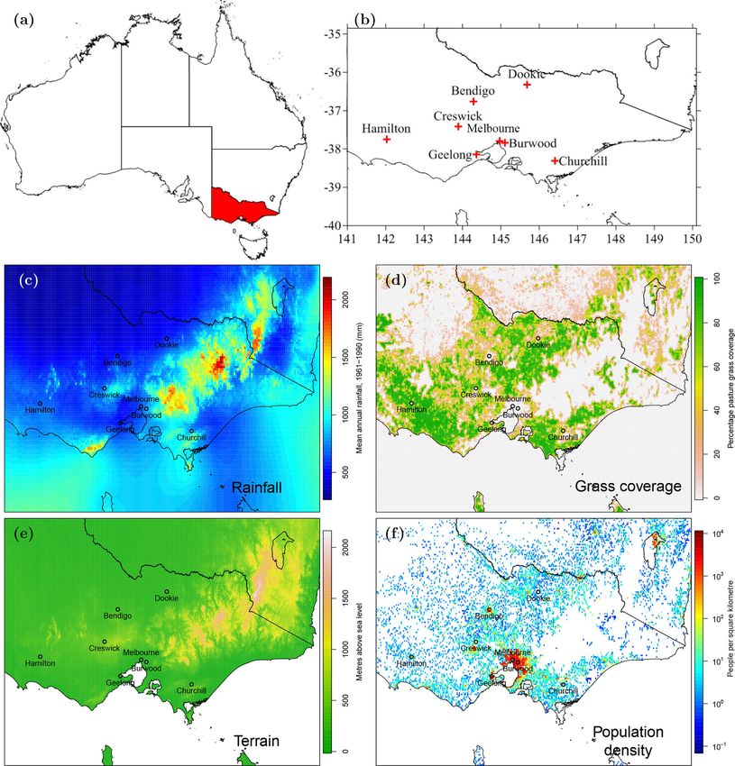
2196                                                        K. M. Emmerson et al.: Victorian Grass Pollen Emissions Module

perienced the world’s largest epidemic thunderstorm asthma          pollen measurements were available. Schueler and Schlun-
event. In the aftermath, the state government funded bet-           zen (2006) simulated oak pollen emission in northern Ger-
ter planning of healthcare resources to improve prepared-           many via the incorporation of landscape structural mapping,
ness and response arrangements for similar events in the fu-        finding that oak pollen plumes were transported up to 100 km
ture (Davies et al., 2017; Lindstrom et al., 2017). This plan       away. The EMPOL 1.0 model for birch pollen across all of
included the development of a pilot thunderstorm asthma             Europe was comprehensively evaluated by Zink et al. (2013).
early-warning service using statistical pollen forecasts (Sil-      The Finnish Meteorological Institute has developed the Sys-
ver et al., 2019), operated by the Bureau of Meteorology            tem for Integrated modeLling of Atmospheric coMposition
(BOM), and the concurrent development of a pollen fore-             (SILAM; Sofiev, 2017, and references therein), to calculate
casting system, built around pollen emission and transport          the concentrations of six pollen species at a 10 km resolution
modelling. The pollen emissions component is called the             on an hourly basis for all of Europe. This group have found
Victorian Grass Pollen Emissions Module version 1.0 (VG-            that the most important input parameter is temperature (Sil-
PEM1.0).                                                            jamo et al., 2013).
   Pollen is generally not included in air quality models be-          Studies of pollen have focused on those taxa with a high
cause its atmospheric lifetime is usually too short to be of        allergenic burden, which differs depending on region. In Eu-
interest. Recently human exposure to pollen has become a            rope, birch tree pollen is the major allergen and has been
focus, particularly in the Northern Hemisphere (e.g. Sofiev         the focus of intense research activity (Siljamo et al., 2013;
et al., 2015; Zhang et al., 2014) and urban areas (Skjøth et al.,   Sofiev et al., 2013; Siljamo et al., 2007; Sofiev et al., 2006).
2013), such that detailed vegetation taxa maps are being pro-       However, birch is not common in Australia. Ragweed pollen,
duced for pollen forecasting (McInnes et al., 2017).                which is a common allergic trigger in the Northern Hemi-
   Techniques to model atmospheric concentrations of pollen         sphere, grows in the north-east and east of Australia but
have included statistical techniques and dispersion mod-            not elsewhere (Bass et al., 2000). Native Australian grasses
els. Statistical techniques using standard multiple regression      such as wallaby and kangaroo grass are generally not wind-
analyses have predicted whether airborne pollen concentra-          pollinated and produce little pollen, whereas introduced agri-
tions will be higher or lower than a long-term mean with            cultural pasture grasses such as ryegrass (Lolium perenne)
> 87 % accuracy (Smith and Emberlin, 2006), but require             and canary grass are high pollen emitters (Smart et al., 1979).
decade-long datasets (Emberlin et al., 2007), and are im-           Ryegrass is grown extensively in Victoria and produces large
proved by the availability of multiple sampling sites. Statis-      volumes of pollen in spring. In southern Australia most of
tical models require a representation of the flowering sea-         the allergenic burden has been attributed to ryegrass via skin
son, but perform poorly if the timing of the flowering season       prick tests (Girgis et al., 2000; Bellomo et al., 1992). Further,
changes (Beggs et al., 2015), whereas in urban areas, they          the rupturing of ryegrass pollen grains releases much smaller
are subject to local-scale turbulence and heat island effects       starch particles that are capable of causing asthma (Taylor
(Emberlin and Norrishill, 1991). Meteorological dispersion          and Jonsson, 2004; Suphioglu et al., 1992). Therefore, VG-
models can capture these effects, but are more computation-         PEM1.0 focuses on pasture grass and has the following goals.
ally demanding to run. Physical dispersion of pollen includes       First, to improve public health emergency planning and re-
(1) emission from the pollen source regions, (2) atmospheric        sponse arrangements around thunderstorm asthma, by pro-
transport and (3) deposition, using measurements to validate        viding a tool for appropriate information providers (i.e. Mel-
the predictions.                                                    bourne Pollen Count and Victorian Department of Health
   Kawashima and Takahashi (1999) were amongst the first            and Human Services). Second, that the VGPEM will feed
to develop a numerical description of pollen within a dis-          into other forecasting models such as BOM’s thunderstorm
persion model, using a flowering map to simulate the cedar          asthma forecast.
pollen season in the Tohoku district of Japan. In the US, the          This paper documents the first representation of grass
Biogenic Emission Inventory System was adapted to emit              pollen in a 3-D dispersion model in Australia. As the great-
birch and ragweed pollen and predicted the timing of the            est uncertainty is in the pollen emission characteristics, we
birch pollen peak to within 2 d (Efstathiou et al., 2011). An       develop and evaluate 10 methodologies, using observations
understanding of pollen release biology and accurate me-            from eight counting sites in Victoria. First we describe these
teorological data are crucial for pollen forecasting (Pasken        grass pollen observations, and determine their correlations
and Pietrowiez, 2005). Wozniak and Steiner (2017) mod-              with observed meteorological variables. Second, the grass
elled pollen from 13 different taxa based on plant functional       pollen emission methodologies are described and tested at
type mapping for the US, which could be used on climatic            a spatial resolution of 3 km. The best performing method is
timescales. Indeed, the climate-induced spread of ragweed is        recommended for VGPEM1.0.
predicted to double the number of Europeans suffering al-
lergic responses by 2060 (Lake et al., 2017). In Germany,
Helbig et al. (2004) simulated hazel and alder pollen emis-
sions and transport, but did not verify their predictions as no

Geosci. Model Dev., 12, 2195–2214, 2019                                               www.geosci-model-dev.net/12/2195/2019/
K. M. Emmerson et al.: Victorian Grass Pollen Emissions Module                                                             2197

2   Observations and characteristics of grass pollen               concentrations. The Australian grass count categories are
                                                                   similar to those used in the UK and Europe for the low and
Despite Australians having high rates of asthma and allergy        medium count categories, but the Australian extreme cate-
compared to other Western nations (Lai et al., 2009), few          gory is reached at pollen counts up to 3 times lower than in
Australian pollen observation sites for routine monitoring or      Europe and the US (Zink et al., 2013; Osborne et al., 2017;
research existed in 2016 (Beggs et al., 2015). In Australia,       US National Allergy Bureau, 2019). Between 20 and 60 d
all pollen sampling is performed using Burkard volumetric          in each Melbourne season are observed in the moderate or
pollen traps (de Morton et al., 2011). Samples are histolog-       above category, and up to 37 d are observed in the high or
ically stained and counted manually under a microscope by          above category (Medek et al., 2016). However, it is clear that
trained personnel who reference the samples to pollen taxo-        climate change is impacting the timing and strength of the
nomic standards. One limitation of this method is that pollen      grass pollen season (Ziska and Beggs, 2012), as are changes
cannot be classified into particular species, or even genus,       to agricultural practices and the expanding boundary of the
based on visual examination alone.                                 city. These changes highlight the importance of long-term
   The University of Melbourne (UoM) operated a pollen             observations and the need to sustain the new pollen observa-
count site in Victoria sporadically from the late 1970s to         tion sites in Victoria.
1990, but since 1991 it has counted annually over the 3-
month period from October to December, coinciding with
the grass pollen season (Ong et al., 1995). In Victoria, rou-      3   Treatment of pollen in VGPEM1.0
tine pollen counting since 2017 distinguishes between 15
pollen taxa, with Haberle et al. (2014) finding that 70 % of       Pollen is set up in VGPEM1.0 as an inert particle tracer.
the total pollen measured at the UoM site is Cupressaceae          The pollen source methodologies are tested using the CSIRO
from a nearby cemetery. However we concentrate on the              Chemical Transport Model (C-CTM), a framework of mod-
Poaceae (grass) pollen, as it is the dominant outdoor hu-          ules designed to calculate the concentrations of gases and
man allergen in Australia. DNA sequencing at the UoM in-           aerosol which are subjected to emission, dispersion and de-
dicates that ryegrass could have contributed 60 %–90 % of          position within the atmosphere (Cope et al., 2009). The C-
the grass pollen counted over the 2016 pollen season (per-         CTM has been used to model the impacts of anthropogenic
sonal communication, E. Newbigin). The amount of grass             emissions on urban air sheds (Chambers et al., 2019; Paton-
pollen during the season in any particular year in Melbourne       Walsh et al., 2018), to model volatile organic compounds
is strongly related to the amount of spring rainfall, which pro-   from vegetation (Emmerson et al., 2019, 2018, 2016) and
motes grass growth and flowering (de Morton et al., 2011).         also to investigate the health impacts of reducing the sul-
The cumulative grass pollen count over the season in Mel-          fur content in shipping fuels (Broome et al., 2016). The C-
bourne ranges between 1500 and 5000 grains m−3 , with daily        CTM is driven by meteorology from the Australian Commu-
maximums reaching 400 grains m−3 (Medek et al., 2016).             nity Climate and Earth System Simulator model (ACCESS,
In Melbourne, the highest pollen counts are usually associ-        Puri et al., 2013), run at a 3 km resolution using boundary
ated with northerly continental air masses (de Morton et al.,      conditions from ERA-Interim for a domain covering Victoria
2011), with an evening peak coinciding with the onset of           (Fig. 1a). ACCESS provides the meteorological parameters
the stable nocturnal boundary layer and descending air (Ong        necessary for pollen emission and transport, namely wind
et al., 1995).                                                     speed and direction, temperature, relative humidity (RH) and
   Two other pollen counting sites close to Melbourne at Bur-      rainfall.
wood and Geelong, which are run by Deakin University, have            Particles are output as micrograms per cubic metre
been in operation since 2012. Five new sites were introduced       (µg m−3 ) in the C-CTM, and require unit conversion to cal-
in 2017 around Victoria and are situated within university         culate grains per cubic metre (consistent with the pollen ob-
or hospital grounds (Fig. 1a, b and Table 1). Pollen sam-          servations), using the mass of one pollen grain. Grass pollen
pling occurred daily during the 2017 grass pollen season at        diameters are found in the range from 30 to 40 µm (Brown
09:00 AEDT , representing the mean daily pollen concentra-         and Irving, 1973). Early calculations by Smart et al. (1979)
tion from 09:00 AEDT the previous day to 08:59 AEDT on             estimated the mass of one ryegrass pollen grain in Melbourne
the day of collection. Pollen observations from these eight        to be 1 × 10⁻⁹ g, which converts to a very low density of
sites are used to assess the accuracy of pollen predictions in     44.5 kg m−3 using a 35 µm diameter. The grass pollen den-
this study.                                                        sity is a large source of uncertainty. Whilst Smart’s study
   In Australia, grass pollen counts are graded “low” if the       is local to our work, studies of pollen from other grass taxa
count is 19 m−3 or less, “moderate” if it is between 20 and        yield much higher densities, for example 980 kg m−3 for Se-
49 m−3 , “high” if it is between 50 and 99 m−3 and “extreme”       cale (rye) (Durham, 1946) and Dactylis glomerata (Stanley
if it is above 100 m−3 . Whilst epidemiological studies com-       and Linskens, 1974).
monly use annual pollen totals, we use a daily pollen risk            The pollen density also impacts on the dry deposition ve-
classification system because we aim to predict daily pollen       locity, which controls the length of time the pollen grain

www.geosci-model-dev.net/12/2195/2019/                                               Geosci. Model Dev., 12, 2195–2214, 2019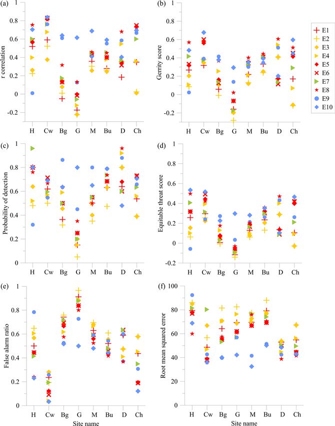
2198                                                         K. M. Emmerson et al.: Victorian Grass Pollen Emissions Module

Figure 1. Maps of (a) Victoria within Australia, (b) pollen observing sites within the domain, (c) mean annual rainfall, (d) pasture grass
coverage, (e) terrain and (f) population density. Data sources: (c) BOM, (d) ABARES, (e) Geoscience Australia and (f) the Bureau of
Statistics.

is airborne. The C-CTM dry deposition parameter follows                   This work relates exclusively to forecasting the presence
Stoke’s law. Sugita et al. (1999) measured Gramineae (grass)           of intact grass pollen grains in the air, within Victoria, Aus-
pollen with a fall speed of 3.5 cm s−1 . Skjøth et al. (2007)          tralia, and does not consider thunderstorm cells or the inter-
suggest the deposition of grass pollen is 4 times larger than          actions of grass pollen grains within them. The process of re-
the 1 cm s−1 estimated for birch pollen, and consistent with           entrainment of pollen grains once they are deposited to the
the 4.3 cm s−1 measured by Durham (1946) on Secale (rye).              ground is not considered, nor is the rupturing process that re-
We will assume that each pollen particle is 35 µm in diam-             leases the allergenic contents of the grains – present on small
eter, spherical and has a density of 1000 kg m−3 , which is            starch particles. Whilst the impacts of pollen rupturing on
consistent with values used by Melbourne-based researchers             numbers of cloud condensation nuclei has been investigated
(de Morton et al., 2011; Knox, 1993), and similar to the grass         by Wozniak et al. (2018), ruptured pollen grains are not rou-
pollen density used in Zhang et al. (2014). A 35 µm particle           tinely monitored in Victoria. Future development of VGPEM
with a density of 1000 kg m−3 yields a deposition velocity             may incorporate some of these processes.
of 4.6 cm s−1 , which is similar to Skjøth et al. (2013). Us-
ing these values, the estimated mass of each pollen grain is
22.4 × 10⁻⁹ g.

Geosci. Model Dev., 12, 2195–2214, 2019                                                   www.geosci-model-dev.net/12/2195/2019/
K. M. Emmerson et al.: Victorian Grass Pollen Emissions Module                                                                         2199

Table 1. Locations of the Burkard pollen sampling network in Victoria arranged west to east, and their nearest automatic weather station
(AWS). Code refers to site names within figures of this paper. UoM refers to the University of Melbourne.

        Site        Code     Long (◦ E)      Lat (◦ S)   Location                                   Closest AWS (distance, km)
        Hamilton    H           142.03         37.74     Hamilton hospital grounds                  Hamilton airport (10.4 km)
        Creswick    Cw          143.90         37.42     UoM satellite campus                       Ballarat aerodrome (15.3 km)
        Bendigo     Bg          144.30         36.78     Latrobe University satellite campus        Bendigo airport (5.5 km)
        Geelong     G           144.36         38.14     Deakin University, Waurn Ponds campus      Geelong racecourse (7.0 km)
        Melbourne   M           144.96         37.80     UoM city campus                            Melbourne Olympic park (3.3 km)
        Burwood     Bu          145.12         37.85     Deakin University, Burwood campus          Scoresby (11.4 km)
        Dookie      D           145.71         36.38     UoM satellite campus                       Shepparton airport (29.3 km)
        Churchill   Ch          146.43         38.31     Federation University campus               Latrobe Valley airport (11.6 km)

3.1     Pollen emissions framework                                        where the terms fh , fRH , fPR , fWS and fTM represent the
                                                                          response to hour of the day, RH, precipitation, wind speed
Pollen emission and transport has never been modelled in                  and temperature, respectively. This approach is similar to
Australia; therefore, we trial three different emission frame-            Sofiev et al. (2013, Eq. 12), representing pollen emissions
works and vary their inputs. In some instances we test param-             from birch trees. The assumption is that grass pollen emis-
eters proven not to work elsewhere and for other pollen taxa,             sions are greatest when conditions are hotter, windier, drier,
to investigate whether Australian ryegrass pollen character-              with less rain and around midday. The midday assump-
istics are different. The first framework is a spatio-temporal            tion stems from an observational study conducted near Mel-
decomposition of factors, the second is a pollen production–              bourne which showed that the peak timing of ryegrass pollen
loss model and the third is a derivative of the statistical model         release (measured as the number of exposed anthers) occurs
for daily grass pollen concentrations used in the BOM’s pilot             in the early afternoon (Smart and Knox, 1979, Fig. 6). As
forecasting system (Silver et al., 2019). The pollen emission             ryegrass flowers in spring when mornings are cool and damp,
rate E at grid-point (x, y) and time t is expressed as follows:           the anthers need to dry before pollen is released. This timing
                                                                          is represented as a Gaussian distribution with a mean at the
E(x, y, t) = I (x, y, t) × G(x, y, t) × S(x, y),                    (1)   local solar noon (12:00 AEDT) and a standard deviation σh ,
                                                                          of either 2 or 4 h (Smart and Knox, 1979). The larger σh pa-
where I is the immediate timing (hour-by-hour variation due
                                                                          rameter allows for a wider peak in pollen around noon in the
to changes in prevailing meteorology), G describes the gross
                                                                          later scenarios E6, E7 and E8.
seasonal timing (also termed the “phenology factor”) and S
                                                                             For RH we adapt the approach of Sofiev et al. (2013), who
provides the spatial source distribution for a given season.
                                                                          used a piece-wise linear relationship scaled from one (RH
The functions I , G and S are each dependent on other fac-
                                                                          of 50 % or less) to zero (RH of 80 % or above). For wind
tors, which may include modelled meteorology, land use data
                                                                          speed, Sofiev et al. (2013) assumed a smaller emission rate
or satellite data; these details are discussed in subsequent sec-
                                                                          (fstagnant = 0.33) in stagnant conditions and scaled smoothly
tions.
                                                                          to a saturation value (1.0) for higher wind speeds. We adapt
   Table 2 gives the combinations of options for calculating
                                                                          this approach to the case of RH, but use a logistic func-
E that are tested in this study. Each emission methodology is                                       1
                                                                          tion (fl (y; α, c) = 1+e−α(y−c)  , for location parameter c and
run for three months between October and December 2017 to
                                                                          rate parameter α), where the rate and location parameters are
cover the period of the pollen measurements. The modelled
                                                                          set to yield fl (50; αRH , cRH ) = 0.95 and fl (80; αRH , cRH ) =
pollen is also averaged on a 24-hourly basis (to 09:00 AEDT
                                                                          0.05, with αRH being negative, meaning that the assumed
each day) to be consistent with the 2017 pollen observations.
                                                                          emissions rate decreases with increasing humidity. The final
3.1.1    Immediate timing (I )                                            fRH is then

We consider two representations of the immediate timing                   fRH = fstagnant + (1 − fstagnant ) · fl (RH; αRH , cRH ).     (3)
function (I ). The first, and simplest, assumes that emissions
are related to transport and are therefore proportional to the                The equation for the temperature term (fTM ) is identi-
surface wind speeds, used in scenarios E1, E2 and E3. The                 cal to the RH term (Eq. 3), but taking temperature (◦ C) as
second method, used in scenarios E4, E5, E6, E7 and E8 ac-                the argument and with different rate and location parame-
counts for several meteorological factors, treating them as               ters. These are defined such that fl (6; αTM , cTM ) = 0.05 and
having independent effects.                                               fl (24; αTM , cTM ) = 0.95. The implied rate parameter (αTM )
                                                                          is positive, meaning that grass pollen emissions are assumed
I (x, y, t) = fh · fRH · fPR · fWS · fTM ,                          (2)   to increase with increasing temperature.

www.geosci-model-dev.net/12/2195/2019/                                                       Geosci. Model Dev., 12, 2195–2214, 2019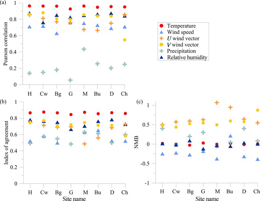
2200                                                          K. M. Emmerson et al.: Victorian Grass Pollen Emissions Module

Table 2. Options tested for pollen emission in this study. EVI denotes the enhanced vegetation index.

                      Scenario   Immediate timing (I )               Gross timing (G)    Spatial function (S)
                      E1         Wind speed                          Gaussian            Grass map
                      E2         Wind speed                          ∂EVI                Grass map
                      E3         Wind speed                          ∂EVI                1.0 (embodied in ∂EVI value)
                      E4         Meteorological function (σh = 2)    ∂EVI                Grass map
                      E5         Meteorological function (σh = 2)    Gaussian            Grass map
                      E6         Meteorological function (σh = 4)    Gaussian            Grass map
                      E7         Meteorological function (σh = 4)    Gaussian            Production–loss model
                      E8         Meteorological function (σh = 4)    Shifted Gaussian    Grass map
                      E9         Statistical model V1                EVI based           EVI based
                      E10        Statistical model V2                EVI based           EVI based

   A similar approach is taken for precipitation (fPR ), with           a normalisation factor of 9.53 × 10⁻⁸ , so that seasonal emis-
the logistic rate and location parameters constrained to                sions integrate to 464 kg ha−1 . This Gaussian representation
satisfy fl (0; αPR , cPR ) = 0.95 and fl (0.5; αPR , cPR ) = 0.05,      is used in scenarios E1, E5, E6 and E7.
where the precipitation is given in units of millimetres per               We apply a second Gaussian representation in scenario
hour (mm h−1 ) and αPR is negative. We cannot impose a con-             E8 which uses the shapes of the 2017 observed pollen time-
straint of the function being 1.0 for zero precipitation, as the        series to shift the distribution by either moving the mean ear-
logistic function approaches 1.0 asymptotically. Instead, we            lier or later in the grass season, and/or adjusting the standard
scale the result based on the function’s value for zero humid-          deviation to be tighter or wider. The curves are fitted by op-
ity (defined above as 0.95), resulting in                               timising the root mean squared error (RMSE) between the
                                                                        pollen counts and the original Gaussian distribution (shown
fPR =fstagnant + (1 − fstagnant ) · fl (PR; αPR , cPR )/                in the Supplement). The peak of the grass pollen season is
        fl (0; αPR , cPR ).                                    (4)      earlier in Bendigo and Dookie than day 46.5, thus all grass-
                                                                        land north of 37◦ S replaces n with 34.7 and σ reduces to
   As noted above, the effect from wind speed (fWS ) is                 15.5 (F remains the same as above). The peaks in observed
assumed to scale smoothly from a lower rate of 0.33 for                 pollen at Creswick and Churchill are later in the season and
fstagnant in still conditions. We follow the parameterisation           count more pollen than other sites; thus, at locations south of
of Sofiev et al. (2013, Eq. 11):                                        37◦ S and east of 143.5◦ E, n is replaced by 50.5, σ is nar-
                                                                        rowed to 19.3 and F increased to 1.2 × 10⁻⁷ . At sites west
fWS = fstagnant +(1−fstagnant )·(1−exp(−WS/Usatur )), (5)               of 143.5◦ E (i.e. Hamilton), the peak of the pollen observa-
                                                                        tions are greater and distributed more tightly, thus n reverts
where wind speeds (m s−1 ) are scaled by a saturation wind              to 48.1, σ is narrowed to 7.7 and F is increased further to
speed (Usatur = 5 m s−1 ), above which the wind speed does              1.56 × 10⁻⁷ .
not promote the release of pollen.
                                                                        3.1.3   Enhanced vegetation index (EVI)
3.1.2    The gross timing (G)

We consider two representations of the gross timing, a Gaus-            Devadas et al. (2018) developed a non-linear statistical model
sian distribution to represent the growth and decline of the            for pollen concentrations using satellite greenness indices
springtime pollen season, and the enhanced vegetation index             across areas surrounding a receptor point. The EVI is a mea-
(EVI). The Gaussian distribution (Eq. 6) is normalised to in-           sure of landscape greenness, which is less affected by satu-
tegrate to the theoretical maximum spatial production of rye-           ration in higher biomass regions than the widely used nor-
grass pollen over the season, estimated by Smart et al. (1979)          malised difference vegetation index (Huete et al., 2002). The
as 464 kg ha−1 of ryegrass pollen in grasslands to the north            EVI value typically increases rapidly with time during spring
of Melbourne.                                                           due to foliage growth in deciduous trees or grass growth.
                                                                        In the Victorian temperate climate, fresh grass rapidly dries
                              (d − n)2                                  (or “cures”) in late spring and early summer, causing a fall

                  F
G(x, y, t) = √          exp −            ,                 (6)          in the EVI. Given the absence of deciduous forests in Aus-
                 2π σ 2          2σ 2
                                                                        tralia, most of the temporal variation in the EVI is due to
where d is the day number (from 1 October to 31 Decem-                  grass growth and curing. Here we investigate a relationship
ber = 92 d) within the season, n is the mean day number of              between the timing of the pollen season and the gradient in
that season (46.5), σ is the standard deviation (26.7) and F is         the EVI over a region in the south-west of Victoria, spanning

Geosci. Model Dev., 12, 2195–2214, 2019                                                    www.geosci-model-dev.net/12/2195/2019/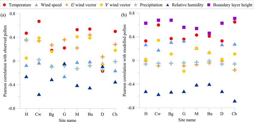
K. M. Emmerson et al.: Victorian Grass Pollen Emissions Module                                                                 2201

37.3–38.3◦ S and 142.0–143.3◦ E (appearing as dashed lines         3.1.4   The spatial function (S)
in Fig. 3). This region is upwind of Melbourne, in terms of
the prevailing climatological wind, and has high agricultural      Mapped grass and pasture for Victoria were extracted from
activity.                                                          the Australian Land Use and Management (ALUM) classi-
   Using the Moderate Resolution Imaging Spectroradiome-           fication (ABARES, 2017) and were re-gridded from a 50 m
ter (MODIS) MOD13C1 data (from the Terra satellite at              resolution to the 3 km grid used by the C-CTM. ALUM in-
0.05◦ resolution), Fig. 2a shows that the gradient in aver-        cludes 193 categories of which only three are assumed to
aged EVI drops off rapidly, around the same time as the            overlap with grazing pastures (“Grazing modified pastures”,
pollen season peaks. Fig. 2b shows that the first derivative       “Native/exotic pasture mosaic” and “Grazing irrigated modi-
of EVI is with the grass pollen time-series at UoM. If we          fied pastures”); the fractional coverage of these three classes
examine inter-annual variation, assessing the day of the year      together is shown in Fig. 1d. We include larger-scale maps of
when the EVI falls most rapidly (represented as the middle         the pasture grass coverage surrounding the pollen count sites
of the 16 d EVI compositing window) and the day of the year        in the Supplement. While many cultivated cropping cereals
when the grass pollen peaks (having first applied a smoothing      grown in the region are also grasses (e.g. wheat and barley),
spline to the pollen time-series), a relationship between these    they are mostly self-pollinating and thus produce very lit-
two quantities is observed: the Pearson correlation is 0.4, the    tle pollen compared with wind-pollinated grass species such
slope of the linear regression is 1.006 and the means of the       as ryegrass. The area to the east of Melbourne is mountain-
two Julian dates differs by only 2.7 d (Fig. 2c). This agree-      ous and therefore not arable (Fig. 1e), whereas the region to
ment is especially notable given the uncertainty induced by        the north-west is arid (Fig. 1c). The most productive areas
the wide EVI compositing window.                                   of pasture grass in Victoria are found in the west of the re-
   Taking this one step further, we apply a similar analy-         gion near Hamilton and south-west of Churchill. The ALUM
sis to each individual 0.05◦ × 0.05◦ MODIS pixel (Fig. 3).         grass map is used in scenarios E1, E2, E4, E5, E6, E7 and E8.
Given the high deposition velocity of grass pollen grains
(4.6 cm s−1 , as discussed above), the contribution of pollen      3.1.5   Pollen production–loss model
emitted from the productive grassland areas in western Vic-
toria to observations recorded in Melbourne is likely to be        In reality, there is a finite amount of grass pollen available for
minimal. However, this analysis may help inform our under-         release at a given time, and once exhausted by in-plant dry
standing about the relationship between the remotely-sensed        and wet deposition, or pollen release, the pollen reservoir is
vegetation index and broad-scale features of the pollen sea-       only replenished at a finite rate. Scenario E7 is a production–
son. The timing of the fall in the EVI in south-west Vic-          loss model for this pollen reservoir.
toria not only correlates well with the timing of the grass
pollen season experienced in Melbourne (Fig. 3a), but the          E(x, y, t) = A(x, y, t) · I (x, y, t)                         (8)
differences in timing are also relatively small (Fig. 3b). The     A(x, y, t) = A(x, y, t − δt) + P (x, y, t − δt)
north-west of the state is generally much drier than the south-    − L(x, y, t − δt)                                             (9)
east (Fig. 1c), and the north-west area dries out earlier in the
                                                                                                                 δt
year (Fig. 3c). Areas identified as crops or pasture (Fig. 1d)     P (x, y, t) = S(x, y, t) · G(x, y, t) ·                      (10)
demonstrate a more rapid fall in EVI (Fig. 3d).                                                                  T
   This exploratory analysis suggests that in this bioclimate      L(x, y, t) = A(x, y, t) · exp(−λ · δt),                      (11)
the broad parameters of the pollen season can be diagnosed
from the EVI fields. On a broad temporal scale, a fall in the      where emissions, E, are set to be the product of the available
EVI over pollen source regions is associated with increasing       pollen reservoir, A, and the instantaneous emission factor,
pollen emissions. In light of this, we consider an EVI-based       I , at grid-point (x, y) and time t. δt is the model time-step.
representation of the gross timing (G):                            The pollen produced, P , is given by the product of the spa-
                                                                 tial and gross-timing terms, proportional to the fraction of
                      ∂EVI(x, y, t)                                the grass pollen season covered between t and t + δt. L is
G(x, y, t) = max 0, −                 .                     (7)
                          ∂t                                       the amount lost between t and t + δt, T is the total length
                                                                   of the grass pollen season and λ is the loss rate due to direct
   The max(·) function ensures that the emissions are strictly     deposition before the pollen leaves the plant. This loss can
positive. We note that Eq. (7) incorporates both temporal and      occur direct to the ground or due to animals brushing past,
spatial information, and can thus be used to represent the         and differs from the in-atmosphere wet and dry deposition
spatial distribution, in which case we can set S = 1.0 for all     rates. Zink et al. (2013) suggest that this loss process is sim-
grid-points (x, y) (scenario E3). Alternatively, we can use the    ilar to a half-life, which we extend to provide a variable loss
same spatial forcing (based on an assumed land use classifi-       rate accelerated in wet conditions. The loss decay parameter
cation) to provide an extra spatial constraint. ∂EVI is used in    (λ), is defined as a piece-wise polynomial function based on
scenarios E2 and E4.                                               the rain rate such that pollen has a half-life on the plant of 2 d

www.geosci-model-dev.net/12/2195/2019/                                                 Geosci. Model Dev., 12, 2195–2214, 2019
2202 K. M. Emmerson et al.: Victorian Grass Pollen Emissions Module
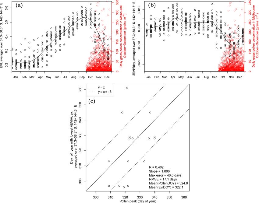
Figure 2. (a) A 16-year climatology in EVI (black) from south-west Victoria (averaged over the region from 37.3 to 38.3◦ S and 142.0 to
143.3◦ E, shown in each panel of Fig. 3) and the grass pollen record in Melbourne (red); the full sequence of data is shown as circles, with a
locally weighted polynomial regression overlaid (Cleveland, 1979). The EVI data are 16 d composites. (b) As in panel (a) except presenting
the derivative of the 16 d EVI with respect to time. (c) The day of the year of the minimum of the ∂EVI
∂ t for each year plotted against the day
of the year of the maximum pollen; when assessing the timing of the grass pollen peak, the grass pollen time-series was smoothed using a
cubic smoothing spline. The dashed lines in (c) represent 16 d either side of a given day, which is the width of the MODIS EVI compositing
window.
in dry conditions and 12 h in wet conditions, with the latter “V2” also used the 2017 data from the eight Victorian sites
corresponding to a rain rate of 2 mm h−1 . (scenario E10). The V1 model was developed ahead of the
2017 pollen season before counts were available at the new
3.1.6 Statistical models pollen sites, as the BOM required input for their pilot thun-
derstorm asthma service. The seasonal component was repre-
In parallel to the emission–dispersion modelling presented sented as a Cauchy distribution (which decays more slowly
here, statistical forecasting methods have been trialled for than a Gaussian distribution), with a fixed scale parameter
use in Victoria. These models are non-linear regression equa- (k = 19 d). The magnitude of the pollen season (correspond-
tions that use weather model data, derived parameters from ing to the maximum of the seasonal term) was estimated
the MODIS EVI and land use maps as predictors. These data by univariate linear regression on the winter-time maximum
can be decomposed into a slow-moving seasonal component EVI. The timing of the seasonal maximum was estimated
(similar to the gross-timing term described above) and a sec- by the day of the year when the EVI falls to 0.05 below
ond component that accounts for day-to-day variation. The its winter-time maximum. The magnitude and timing were
models were trained on daily pollen count data, and thus can- smoothed spatially using an inverse cubed distance weight-
not resolve higher-resolution temporal variation. The gross- ing.
timing function smooths out much of the day-to-day varia- Both V1 and V2 were constructed as generalised additive
tion, and is modulated by the immediate-timing term when models (Wood, 2006), a form of multivariate regression that
estimating temporal variability in the emissions module. The allows for a non-linear influence of the predictor variable on
two statistical models are described in detail in Silver et al. the response variable. The response variable used was the
(2019), and summarised here. “V1” used data from Mel- log(x + 1)-transformed pollen count. The log of the Cauchy
bourne spanning from 2000 to 2016 (scenario E9), whereas
Geosci. Model Dev., 12, 2195–2214, 2019 www.geosci-model-dev.net/12/2195/2019/K. M. Emmerson et al.: Victorian Grass Pollen Emissions Module 2203
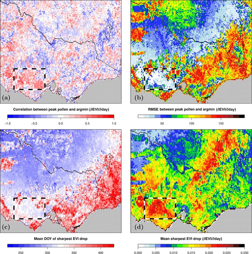
Figure 3. Relationship between the timing of the peak in grass pollen in Melbourne and the timing of the sharpest drop in EVI at each
MODIS pixel: the correlation (a) and the root mean squared error in the timing (b). Also shown are the average timing (c) and rate (d) of
the fastest fall in EVI at each point in the domain. The dashed rectangle in south-west Victoria (spanning 37.3–38.3◦ S and 142.0–143.3◦ E)
displays the region over which the EVI time-series were averaged for Fig. 2. “argmin” refers to the minimum argument.
term and a number of derived weather parameters were con- The statistical models were adapted for 3-D dispersion
sidered for inclusion in the model. Each model was built modelling to use hourly meteorological inputs (or daily, in
up via forward step-wise variable selection; starting with a the case of precipitation). The adapted forms of the two mod-
“null model” (predicting nothing but the mean), terms were els are as follows:
considered for inclusion. Each predictor was trialled as hav-
ing a linear or alternatively non-linear effect on the response log(1 + P1 (x, y, t)) = −0.290 + 0.970 · R1 (x, y, d)
variable, and the out-of-sample prediction skill was tested. − 0.183 · log(PR(x, y, d) + 1) − 0.117 · log(PR(x, y, d))
The combination of predictor and form (i.e., linear or non-
+ fTM1 (x, y, t) + fRH1 (x, y, t) (12)
linear) that yielded the biggest gain in predictive skill was
retained. This procedure was repeated until the incremental log(1 + P2 (x, y, t)) = 1.225 + 0.770 · R2 (x, y, d)
impact of additional terms on predictive skill was negligible. − 0.033 · WS(x, y, t) + fRH2 (x, y, h)
The model skill was tested by leaving out entire pollen sea- + fTM2 (x, y, t) + fPR (x, y, d), (13)
sons, fitting the model without these data, then assessing the
model using the out-of-sample subset. Model skill was quan- where P is the predicted pollen emission for version i at grid-
tified using the Pearson correlation between predicted and point (x, y) and time t, Ri is the seasonal term based on the
observed pollen. EVI parameters at grid-point (x, y) and for day d (outlined
www.geosci-model-dev.net/12/2195/2019/ Geosci. Model Dev., 12, 2195–2214, 20192204 K. M. Emmerson et al.: Victorian Grass Pollen Emissions Module
below), and WS is the wind speed (m s−1 ). In both versions of Table 3. The 2 × 2 contingency table describing each model out-
the statistical model, the variable selection process assigned come. The model outcomes a, b, c and d then become the variables
a non-linear response to the temperature, fTMi (◦ C) and RH in Eqs. (20)–(23).
fRHi (%). Only V2 uses a non-linear term for daily precipita-
tion, fPR (mm). The non-linear relationships between pollen Observation
emission and increasing temperature, RH and precipitation Model Yes No
are shown in Fig. 4. The shaded regions correspond to plus Yes (a) Hit (b) False alarm
or minus twice the standard error of the GAM term, and are No (c) Miss (d) Correct negative
greater in regions of the distribution with fewer observations.
For example, there were far fewer observations at the upper
tail of the temperature range considered, and the standard er- 2019, for further details). The statistical approach accounts
rors are correspondingly larger. for inter-annual variation via the EVI time-series at each grid
The statistical parameterisations were based on ambient cell. Higher winter-time peak EVI values are associated with
pollen concentrations rather than emissions; thus, the non- higher cumulative grass pollen counts over the following sea-
linear terms take transport and dilution processes into ac- son.
count. The shapes of these relationships are similar to those
described by Erbas et al. (2007) for grass pollen in Mel- 3.2 Statistical evaluation
bourne, and also by Zink et al. (2013) for birch pollen in
Europe. The temperature response in both models increased The skill of the pollen forecasts depends in part on how well
until 25 to 30 ◦ C (Fig. 4a, c). The decline in pollen response the meteorology is predicted. The Pearson correlation indi-
at higher temperatures is likely due to dilution with higher cates the strength of the correspondence without considera-
planetary boundary layers. On days in November where the tion of differences in magnitude, whereas the index of agree-
temperature is above 25 ◦ C, the maximum modelled bound- ment (IOA, described in the Supplement) is a good indica-
ary layer height is nearly double the height modelled on days tor of model performance. The normalised mean bias (NMB)
below 25 ◦ C. Thus, the assumption of declining emissions gives the relative difference between the model and observa-
with increased temperature is likely incorrect. There is rel- tions.
atively little non-linearity with humidity. The general trend To determine the best pollen emission methodology, we
is for increased concentrations (or emissions) in drier con- look for skill in the ability of VGPEM1.0 to forecast the pos-
ditions, explained by the drying required before anther de- sibility of the pollen being classed as high or extreme (> 50
hiscence. The rainfall term shows a sharp decline until about grains m−3 ), which is a level at which health impacts may be
2 mm d−1 , after which little additional pollen suppression oc- felt more strongly. The number and timing of predicted high
curs, although there is considerable uncertainty given the rel- pollen days is evaluated quantitatively for consistency and
ative paucity of high-rainfall days. The suppression of grass accuracy, by calculating the probability of detection (POD),
pollen concentrations (or emissions) is likely due to the low the false alarm ratio (FAR) and the equitable threat score
potential for anther dehiscence in moist conditions, and the (ETS) from a simple table of model outcomes (Table 3). The
wet deposition of ambient pollen. POD is the fraction of correctly identified high model fore-
The seasonal term based on the EVI parameters is given as casts compared with the observations, between zero and one:
Ri (x, y, d) = log(SFi (x, y) · fC (d, µi (x, y), k)), where (14) a
POD = . (20)
" #!−1 a+c
d −µ 2
fC (d, µ, k) = π · k · 1 + (15)
k
The FAR puts a value between zero and one regarding how
SF1 (x, y) = max(−4355.913 + 21490.343 many of the predicted high pollen days did not correspond
· Emax,smoothed (x, y), 10−10 ) (16) with an observed high pollen day:
µ1 (x, y) = Edrop,smoothed (x, y) (17) b
FAR = . (21)
SF2 (x, y) = 267.627 + 8853.990 · Emax,smoothed (x, y) (18) a+b
µ2 (x, y) = 202.478 + 0.385 · Edrop,smoothed (x, y), (19) The ETS is the fraction of modelled high pollen days that
where the scale factor parameter SFi (x, y) is based on were correctly predicted and is adjusted for correctly mod-
the smoothed value of the winter-time maximum EVI elled days occurring with random chance. The ETS value is
(Emax,smoothed (x, y)), whereas the timing of the peak of the between −1/3 and 1, with a score of 0 indicating no skill;
pollen season (µi (x, y)) is assumed to scale linearly with this is defined as
the smoothed field of the day of the year when the EVI a − arandom
drops 0.05 below its winter-time maximum (see Silver et al., ETS = , (22)
a + b + c − arandom
Geosci. Model Dev., 12, 2195–2214, 2019 www.geosci-model-dev.net/12/2195/2019/K. M. Emmerson et al.: Victorian Grass Pollen Emissions Module 2205
Figure 4. The shape of the non-linear terms in the statistical models related to temperature (a and c), relative humidity (b and d) and rainfall
(e) for V1 (a and b) and V2 (c, d and e). The shaded regions correspond to plus or minus twice the standard error of the GAM term.
where 4 Results and discussion
(a + c) × (a + b) 4.1 Verification of meteorology
arandom = . (23)
a+b
Meteorological variables are extracted from the ACCESS
As Zink et al. (2013) point out, low skill scores are given
runs at the locations of the AWSs closest to the pollen obser-
to models where the pollen concentrations are close to ob-
vation sites (Table 1). At some pollen observation sites the
served concentrations yet fall into separate “risk” categories.
AWSs are located more than 10 km away, or nearly 30 km
For example, the model predicts 48 grains m−3 and classes
away in the case of Dookie. A direct comparison is made of
the risk category as “moderate”, whereas the observations
hourly temperature, wind speed, wind vectors, precipitation
are 52 grains m−3 and the risk category is “high”. There-
and RH between ACCESS and the AWS observations, us-
fore, we also evaluate the modelled pollen against the ob-
ing the Pearson correlation, IOA and NMB. (Fig. 5). Here
servations in terms of their Pearson correlation, RMSE and
the NMB is normalised by the mean of the absolute value
Gerrity score. Statistical evaluations using categorised and
of the observations (as opposed to the mean of the observa-
non-categorised pollen counts will show how the Australian
tions) because wind vectors contain negative values. Tem-
grass pollen thresholds impact our results. The Gerrity score
perature and RH are both modelled with a high degree of
puts a value on the accuracy of VGPEM1.0 in predicting all
accuracy at all sites, demonstrating a high Pearson correla-
of the observed pollen categories, relative to that of random
tion (average r = 0.9), almost no bias, and high IOA (average
chance (Gerrity, 1992). Gerrity scores range between −1 and
IOA = 0.8). Predicted wind speeds are biased slightly low
1, with 0 indicating no skill and 1 being a perfect model. Cal-
(average NMB = −0.2). The V (north–south) component is
culation of Gerrity scores is complex and is described fully
approximately as well modelled as the U (east–west) compo-
in the Supplement.
nent (average V r = 0.80 compared to average U r = 0.77).
The best forecasting methodology will have a high Pear-
Precipitation has a low degree of bias (average NMB = 0.17)
son correlation, Gerrity score, POD and ETS, and a low FAR
but is not particularly well correlated with the observations
and small RMSE.
(average r = 0.21), and has a lower overall IOA (average
IOA = 0.55).
www.geosci-model-dev.net/12/2195/2019/ Geosci. Model Dev., 12, 2195–2214, 20192206 K. M. Emmerson et al.: Victorian Grass Pollen Emissions Module
4.2 Observed and modelled pollen correlations with 4.3 Verification of pollen source methodologies
meteorology
The modelled pollen concentrations are first normalised by
We assess which measured AWS meteorological variables the observed seasonal mean across all observation sites,
are most strongly related to the observed pollen. Figure 6a which is equal to 47 grains m−3 . This normalisation allows
shows that observed grass pollen is most strongly corre- the evaluation of trends in the daily grass pollen concen-
lated with temperature at the majority of sites (average r = trations without considering their magnitude, as this can be
0.44), and most negatively correlated with RH (average r = corrected later. For 2017, observed individual site means
−0.34). range from 31 grains m−3 at Melbourne to 60 grains m−3 at
Observed wind speed is not strongly related to observed Creswick. The lowest means are found in the densely pop-
grass pollen, except when combined with direction, specif- ulated regions of Geelong, Melbourne and Burwood (see
ically the U wind vector is generally a stronger predictor Fig. 1f). Figure 7 shows correlations and statistical results
of pollen (average r = 0.32) than the V wind vector (aver- for each pollen observation site. Numbers of observed days
age r = 0.22). We include a wind rose for each AWS site in in the lumped high and extreme category (> 50 grains m−3 )
the Supplement to determine the strength of the winds. The are above 20 d for all sites.
roses show a strong southerly influence, corresponding with E1, E2 and E3 used wind speed as the immediate timing
an afternoon sea breeze at most sites apart from Churchill, lo- function, which provided poor prediction skill scores (aver-
cated within an east–west aligned valley. Sites further west in age r = 0.25, 0.18 and 0.17 respectively), similar to results
Victoria (Hamilton and Creswick) also show a northerly in- by Viner et al. (2010) and Zink et al. (2013). Wind pro-
fluence, generally with a greater percentage of wind speeds motes pollen emissions, but the plant must flower first – a
above 4 m s−1 than elsewhere. Precipitation washes pollen process not controlled by wind speed. Wind also correlates
from the air, but shows no correlation here as rain during poorly with pollen observations due to the competing effects
the 2017 season was infrequent (average r = 0). Pollen ob- of strength versus increased ventilation and mixing (Sofiev
servations at Dookie are the least correlated with any of the et al., 2013). Subsequent method E5 used the meteorolog-
meteorological variables, perhaps because the closest AWS ical timing function that included temperature and RH and
is 29 km away. performed better (average r = 0.43). Sofiev et al. (2013) also
Figure 6b shows Pearson correlations for the modelled showed that observed birch pollen in Europe was negatively
pollen against ACCESS meteorology, using scenario E8 as correlated with RH. Widening the timing of the peak pollen
an example that uses the meteorological timing function. emission from 2 to 4 h, as included in E6, improved results
The strengths of the modelled correlations are broadly sim- further over E5 (average r = 0.44).
ilar to those observed in Fig. 6a, but the model is more At most sites the Gaussian description of the season per-
strongly coupled to wind speed (average r = 0.25) and less formed better than the ∂EVI, shown by improvements in the
correlated with the U wind vector than is observed (aver- FAR of E1 over E2, both of which used wind speed as the
age r = −0.07). However, the observed U and V correla- immediate timing descriptor (average FAR = 0.57 and 0.61
tions are not strong, and do not point to particular loca- respectively), and E5 over E4, both of which used the me-
tions being strong pollen sources. Inverse modelling may teorological timing function (average FAR = 0.48 and 0.52
help pinpoint productive grass pollen regions for each site. respectively). These results indicate that using ∂EVI data
We extracted the boundary layer height from the model (un- as descriptors of the pollen season results in poor skill at
available in the observations), which showed that the mod- most of the sites. The ∂EVI data are very noisy. However,
elled grass pollen is more strongly correlated with atmo- E4 using the ∂EVI data and a meteorological timing func-
spheric dilution (average r = 0.61) than it is to tempera- tion gives a good Gerrity score (0.54) and high POD (0.92)
ture (average r = 0.44). Average modelled diurnal bound- and ETS (0.40) at Dookie. When other elements of the EVI
ary layer evolution during November 2017 in Melbourne in- data are used in the statistical models (E9 and E10), such
creases after sunrise at 05:00 AEDT to a peak of 1780 m at as the winter maximum and the day on which the EVI falls
13:00 AEDT. The height declines during the afternoon coin- below 0.05 of the winter maximum, the pollen prediction is
cident with a southerly sea breeze, but is still above 1200 m at much improved at most sites (average POD E9 = 0.67 and
17:00 AEDT. The nocturnal boundary layer is around 200 m. E10 = 0.69). The performance of E10 indicated improve-
Over 77 % of grass pollen is found at ground level (Damialis ments in forecasting skill at all sites with the exceptions
et al., 2017) due to its size and density. The lifetime of our of Dookie and perhaps Bendigo. E10 predicted the lowest
model pollen over 1 km is 6 h. The model RH is more nega- FAR of high pollen predictions at five of the eight observa-
tively correlated with grass pollen levels (average r = −0.52) tion sites (average FAR = 0.37). The ETS adjusts the model
than is observed. The observed relationship may be weaker, score for achieving high pollen predictions at random. E10
as the pollen measurements are not coincident with the AWS. achieves higher ETS scores at four of the eight sites (average
ETS = 0.35). Both the statistical emission parameterisations
assume an underlying Cauchy distribution, which is modu-
Geosci. Model Dev., 12, 2195–2214, 2019 www.geosci-model-dev.net/12/2195/2019/K. M. Emmerson et al.: Victorian Grass Pollen Emissions Module 2207 Figure 5. Comparison of observed and modelled meteorological variables at automatic weather station sites nearest to the pollen observation sites. (a) Pearson correlation. (b) Index of agreement. (c) Normalised mean bias. Figure 6. Pearson correlations of (a) observed pollen with observed meteorological variables from the nearest automatic weather station, and (b) modelled pollen with modelled meteorological variables. lated by the effects of wind, temperature, RH and rainfall. elsewhere with high FAR and RMSE scores at the other ob- At each model grid cell, the peak and magnitude of this bell servation sites (average FAR = 0.55 and RMSE = 63). E7 curve is calculated from statistics inferred from the EVI gra- used the Gaussian distribution for the seasonal term which dient. could be improved upon, but the method was superseded by The pollen production and loss model E7 had a very high the good performance of the statistical models (with the ex- POD (0.96) at Hamilton, but the method was less effective ception of E9 in Hamilton and Geelong). www.geosci-model-dev.net/12/2195/2019/ Geosci. Model Dev., 12, 2195–2214, 2019
2208                                                          K. M. Emmerson et al.: Victorian Grass Pollen Emissions Module

Figure 7. Results from the pollen emission methodology scenarios: (a) Pearson correlation, (b) Gerrity score, (c) POD, (d) ETS, (e) FAR
and (f) RMSE. The sites are presented from west to east, and red refers to Gaussian methodologies, yellow refers to ∂EVI methodologies,
green refers to the production–loss model and blue refers to statistical methodologies. A higher score is better for the Pearson correlation,
Gerrity score, POD and ETS. A lower score is better for the FAR and RMSE.

   The Geelong pollen observations are not well modelled                 for Geelong shows the strong Southern Ocean influence, and
by most of the emission methodologies with Gerrity scores                there are few grass-filled pixels between the coast and the
mainly in the negative region and high FAR > 0.8. E10 pro-               pollen count site which the model relies upon (Supplement).
vides the best scores by far at Geelong with a 0.62 Pearson                 The sites vary considerably in terms of surrounding
correlation and 0.3 Gerrity score, although, overall, results            land use, whereas all of the pollen in the model comes
are poorer for Geelong than any other site. The wind rose                from pasture grass. This impacts the individual site perfor-

Geosci. Model Dev., 12, 2195–2214, 2019                                                     www.geosci-model-dev.net/12/2195/2019/
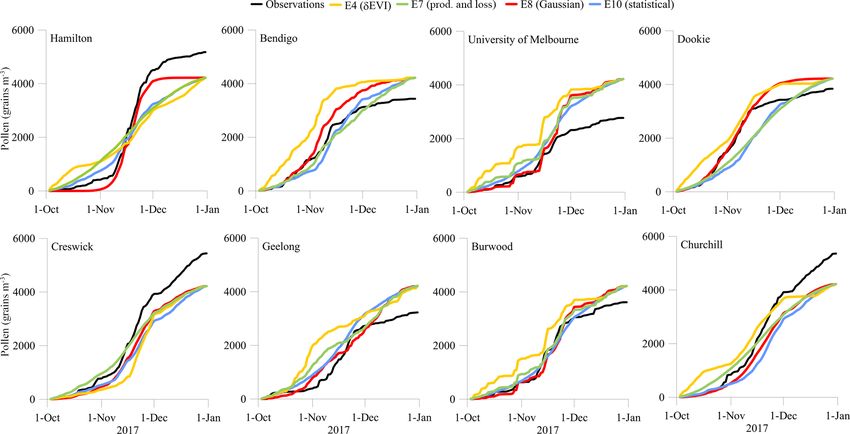
K. M. Emmerson et al.: Victorian Grass Pollen Emissions Module                                                              2209

mance against the pollen observations. Hamilton, Dookie             other regional sites, perhaps indicating more atmospheric
and Churchill are close to pollen source areas. Creswick is         variability near the coasts. It might also indicate the larger
surrounded by forest. The Burwood and UoM sites are in              distances between the urban sites and the grass pollen pro-
heavily built up areas with green space, which is not included      duction regions (more transport and less local production),
in the model pasture grass maps.                                    compared with the monitoring sites within grass pollen pro-
   Comparing the results of the non-categorised Pearson cor-        duction areas (less transport and more local production).
relation and RMSE against the categorised Gerrity score             Here we also note the apparent lack of an “S” shape in the
yields minor differences between 0.1 and 0.2 units, and sug-        modelled profiles at Geelong, which may account for the
gests that the Australian grass pollen thresholds influence         poor model performance at this site.
the analysis by about 15 %. If the best performing scenario            Table 4 splits the best model predictions from E8 and
for each observation site and under all scoring methods is          E10 into low, moderate, high and extreme categories for di-
counted from Fig. 7, shifted Gaussian methodology E8 is             rect comparison with observed categories. Here data from
best 12 times, statistical representation E9 is best 4 times and    all counting sites are combined to ensure a large sample
E10 is best 25 times. E9, built using data prior to the 2017        size. The diagonal in each table highlights the number of
season, has a stronger dependence on precipitation than E10,        days the model has correctly predicted the observed cate-
which is not supported by the correlation of 2017 pollen with       gory. Values far from the diagonal indicate the model has
meteorology. This suggests that the V2 statistical approach to      under- or over-predicted the observed pollen. We want to
the immediate timing combined with an EVI-based approach            avoid occasions where the observed pollen is extreme, but
to the gross timing and a spatial source is likely to produce       the model predicts low pollen. Table 4 shows that both E8
the most accurate pollen forecasts.                                 and E10 have good skill in predicting low observed pollen
   It is useful to plot the observed and modelled pollen as         days. Both models also show high occurrences of predict-
a cumulative time-series, as this indicates the timing of in-       ing moderate pollen when the observed category is low. Sil-
creased and decreased pollen counts (Fig. 8). Here we focus         jamo et al. (2013) found difficulties in modelling moderate
on the best performing scenarios from each of the seasonal          category days, which is not the case here. Both models are
emission methods, capturing the range in descriptions of the        equally good at predicting the high and extreme observed
pollen season. The observations show an “S” shaped profile,         categories. E10 has fewer occurrences of predicting extreme
with increased pollen gradients in November. By the end of          pollen on days when observations were low than E8. How-
the 2017 season, all modelled profiles reach a cumulative to-       ever, there are six cases in E8 and one in E10 that pre-
tal of 4200 grains m−3 due to normalisation to the same ob-         dict low pollen when the observations are extreme. These
served mean value.                                                  cases occur around the 10–11 November within the city at
   The ∂EVI method E4 tends to emit grass pollen too early          Geelong, Melbourne and Burwood. Examining the meteo-
in the season compared with observations at most sites. How-        rology from this period (pollen counts are date-stamped at
ever at Dookie the shape of the season in E4 and E8 is              09:00 AEDT, but represent the preceding 24 h) shows that the
more similar to the observations, and E4 captures the mid-          model has captured the observed temperature, wind speed,
November change when pollen counts decrease better than             direction and zero rainfall. The observed wind direction is
E10. The observed pollen at Dookie experienced a much               from the south and south-east, bringing mainly clean, ma-
larger grass pollen input from the middle of October to             rine air. However observed pollen is extreme on these days,
early November than E10 (but is represented well by E8).            suggesting a highly localised source. One explanation is that
There is little additional observed pollen at Dookie after early    only pasture grass is considered in the model, whereas grass
November, which is at least 20 d earlier than at the other sites.   is usually present in most other land use categories. There
At Melbourne, Bendigo and Burwood, both E8 and E10 pre-             is green space within most cities on both public and pri-
dict the early part of the grass pollen season very well, but       vate land, and grass plants are efficient at colonising dis-
emitted too much modelled pollen towards the end of the             turbed areas such as road verges. Correlations between ob-
season. The steeper gradient in E8 and E10 at Melbourne             served pollen at each site are not particularly strong (aver-
between the middle and the end of November shows that too           age r 2 = 0.28), suggesting that the pollen sources may not
much pollen was emitted during this period. In contrast, ob-        be related, or are highly localised. The modelled correla-
served pollen at Churchill, Creswick, and Hamilton shows a          tions between all sites are very strong because they share the
rapid increase in emissions at the end of November that is not      same pollen source characteristics (average r 2 = 0.80). In-
matched by either E8 or E10. However, the observations sug-         verse modelling could highlight where other grass land use
gest that additional pollen continues to be emitted towards         categories contribute to grass pollen. Future development of
the end of December at Creswick and Churchill, prolonging           VGPEM could consider the sub-grid-scale grass fraction us-
the season. Scenario E8 captures the steep November gradi-          ing high-resolution satellite data sources.
ent at Hamilton very well.
   The observed and modelled pollen cumulative profiles in
Melbourne, Geelong and Burwood are less smooth than the

www.geosci-model-dev.net/12/2195/2019/                                                Geosci. Model Dev., 12, 2195–2214, 2019
You can also read