Inferring ecosystem networks as information flows - Nature
←
→
Page content transcription
If your browser does not render page correctly, please read the page content below
www.nature.com/scientificreports
OPEN Inferring ecosystem networks
as information flows
Jie Li1,2 & Matteo Convertino1,2,3,4*
The detection of causal interactions is of great importance when inferring complex ecosystem
functional and structural networks for basic and applied research. Convergent cross mapping (CCM)
based on nonlinear state-space reconstruction made substantial progress about network inference
by measuring how well historical values of one variable can reliably estimate states of other
variables. Here we investigate the ability of a developed optimal information flow (OIF) ecosystem
model to infer bidirectional causality and compare that to CCM. Results from synthetic datasets
generated by a simple predator-prey model, data of a real-world sardine-anchovy-temperature
system and of a multispecies fish ecosystem highlight that the proposed OIF performs better than
CCM to predict population and community patterns. Specifically, OIF provides a larger gradient of
inferred interactions, higher point-value accuracy and smaller fluctuations of interactions and α
-diversity including their characteristic time delays. We propose an optimal threshold on inferred
interactions that maximize accuracy in predicting fluctuations of effective α-diversity, defined as the
count of model-inferred interacting species. Overall OIF outperforms all other models in assessing
predictive causality (also in terms of computational complexity) due to the explicit consideration of
synchronization, divergence and diversity of events that define model sensitivity, uncertainty and
complexity. Thus, OIF offers a broad ecological information by extracting predictive causal networks
of complex ecosystems from time-series data in the space-time continuum. The accurate inference
of species interactions at any biological scale of organization is highly valuable because it allows to
predict biodiversity changes, for instance as a function of climate and other anthropogenic stressors.
This has practical implications for defining optimal ecosystem management and design, such as fish
stock prioritization and delineation of marine protected areas based on derived collective multispecies
assembly. OIF can be applied to any complex system and used for model evaluation and design
where causality should be considered as non-linear predictability of diverse events of populations or
communities.
“But truth is ever incoherent”
Astrid Recker.
Ecosystem complexity and predictability. The flourishing development of complexity science1, 2 has
shed light on research questions and applications in many interdisciplinary fields, for instance, climate c hange3–5,
epidemiology6, 7 and ecosystem sciences at multiple scales8–10. In this burgeoning science, complex network
models play a central role in the quantitative analysis, synthesis and design (including predictions) of ecosystems
and their visual representation. This is because functional and structural networks—such as species interac-
tions and ecological corridors—are the core elements of ecosystems defining species organization and ecosystem
function. When inferring networks, causal inference11 is one of the fundamental steps for ecosystem reconstruc-
tion and graphical representation by assessing interactions or interdependencies dynamically or across a period
of time—between biota, environment, and among those—that can be conceptualized as information flows in
a general purview12. In a quantitative sense, network inference can performed via causality inference based on
time series data defining the dynamics of ecosystem components. Causal inference also attracts much attention
1
Nexus Group, Faculty and Graduate School of Information Science and Technology, Hokkaido University, Sapporo,
Japan. 2GI‑CORE Global Station for Big Data and Cybersecurity, Hokkaido University, Sapporo, Japan. 3Graduate
School of Information Science and Technology, Hokkaido University, 9 Chome, Kita 14, Nishi 9, Kita‑ku, room
11‑11, Sapporo, Hokkaido 060‑0814, Japan. 4Institute of Environment and Ecology, Tsinghua Shenzhen
International Graduate School, Tsinghua University, Shenzhen, China. *email: matteo@ist.hokudai.ac.jp
Scientific Reports | (2021) 11:7094 | https://doi.org/10.1038/s41598-021-86476-9 1
Vol.:(0123456789)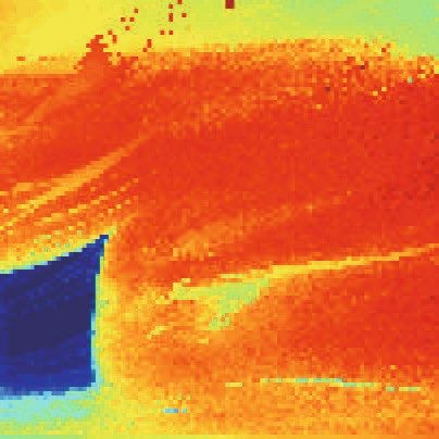
www.nature.com/scientificreports/
in some emerging disciplines such as big data science via machine learning since it brings a new set of tools and
perspectives for some problems in these areas. However, this issue of causal inference is still an extremely chal-
lenging problem due to the intrinsic lack of knowledge or observability of the “true” reality of a system especially
for highly complex non-linear systems driven by non-linear environmental forcing. Certainly the objective of
causal inference is defining unknowns; however robust model validation must be performed. In order to make
causal inference practical and achievable, causality is often replaced with predictability as it is articulated in this
paper. A plethora of conceptual approaches, frameworks and algorithmic tools including but not limited to Pear-
son’s correlation coefficient (PCC)13, 14, Bayesian networks (BNs) and dynamic Bayesian networks (DBNs)15–19,
neural networks, graphical Gaussian models (GGMs)20, 21, Wiener–Granger causality (GC) m odel22, structural
equation modeling (SEM)23–28, convergent cross mapping (CCM)29 and information-theoretic models30–33 for
instance, to tackle causal interactions and infer complex networks in terms of correlation, predictability and
probability have been well established; however, most tools are solely tested on low-dimensional systems and
some are even untested on ecosystems at different levels of complexity or simulated ones. The vast majority of
these models in ecosystem science (with the exception of CCM and few others such as P CMCI34) consider only
the inferred causality between species pairs one at a time without the simultaneous consideration of all species
pairs for each species that is shaping ecosystem collective behavior mediated by environmental dynamics. The
ensemble of all species causations is representable as nonlinear dynamical network over the space-time-envi-
ronmental domain considered. It is therefore valuable for science to seek for robust models and explore novel
methods to identify and quantify the pattern-oriented causality between variables (such as species) and how this
causality is predictive of target complex system patterns.
Causal interaction inferential models. From granger to convergent cross mapping. For quite a long
time, correlation has been considered as a heuristic of causal relationship between variables even though George
Berkeley35 always suggested that correlation did not necessarily or sufficiently imply causation. Especially for
ubiquitous nonlinear dynamics, applying linear correlation to infer causation is cursory and risky. Statements
about causation and correlation actually do not have much to do with each other, particularly when there is no
a-priori knowledge of the studied ecosystem processes. The conceptualization and identification of “causality”
was originally introduced by Wiener36 who propounded that “causality” between two variables can be identified
by measuring how well one variable facilitates the predictability of the other. In this broader view causality was
already conceptualized correctly as predictability.
In 1969, Granger formalized Wiener’s idea36 in terms of autoregression and established the framework of
Wiener-Granger causality (GC) model22 that after led to the Nobel prize in economics. Since then, GC approach
has become a frequently used advance for causation and useful to infer causal interactions between strongly
coupled variables. According to the concept of GC model, a variable is said to “GC cause” a second variable if
knowledge of the current value of the first variable helps in predicting that of the second variable. This notion
of causality was substantially based on the predictability of time series, although strictly speaking Granger
causality is about conditional independence of variables rather than predictability. The key requirement of GC
model is separability that is a feature of purely linear and stochastic systems22, and provides a way to understand
the system as sum of components rather than as a whole non-linear entity composed by multiple components
difficult to separate. Separability means that the second variable can be independently and uniquely forecasted
by the first variable; an assumption that reflects how studied systems are interpreted as linear systems and that
is certainly not the case of real complex systems. Additionally, states in the past of some variables in dynamical
systems can be inherited through time, which means that the behavior of dynamical systems has memory. Yet,
both cause and effect are embedded in a non-separable higher dimension trajectory. Space-time separability
therefore becomes extremely hard to satisfy in systems that can be described as complex networks where each
node (variable) influences several nodes or even all nodes in the entire system simultaneously, resulting in a
non-random propagation of information through the network. In this sense ecosystems can be thought that
information machines where separability is only possible by fixing thresholds of significance for the patterns to
investigate. As a consequence, GC model might be problematic while using in nonlinear dynamical systems with
deterministic settings and weak to moderate interaction. In attempt to solve the causality inference problem in
complex ecosystems, Sugihara et al.29 developed the convergent cross Mapping (CCM) m odel29, and successfully
applied this model to a coupled non-linear mathematical predator-prey model and a real-world sardine-anchovy-
temperature ecosystem. Later on, Ushio et al.37 applied CCM to a complex fish ecosystems with 15 species after
removing seasonality from abundance data in order to assess “true” or biological interactions.
In dynamic systems two variables (X and Y for instance) are causally linked if they are generated by one
system and share a common attractor manifold. It implies that each variable can be used to recover (predict) the
other one. CCM is the method capable of quantifying this kind of correspondence between two variables. CCM
does so by measuring the extent to which the states of one variable (considering values rather than probability
distributions) can be reliably estimated by the other one with time lags. In practice, CCM take values of variables
X and Y, a time lag embedding is derived from the time series of Y, and the ability to estimate the states of vari-
able X from the time lag embedding quantifies how much signature of X is encoded in the time series of Y. This
principle was termed as “Cross Mapping”, and it was suggested that the causal effect of X on Y is determined by
how well Y “cross maps” Sugihara et al.29 noted that CCM had drawbacks, although some of these are disputable.
For instance for the phenomenon of “generalized synchrony” as a result of exceptionally strong unidirectional
causation (X strongly “cross maps” Y, but Y does not causes X). In such a case, both directions (X “cross maps”
Y, Y “cross maps” X) of the causal relationship can be observed from CCM’s results, resulting in a “misleading”
bidirectional causality38. This was perceived as a limitation of CCM in distinguishing between bidirectional cau-
sality and strong unidirectional causality because of the synchrony. Misleading is however not a correct definition
Scientific Reports | (2021) 11:7094 | https://doi.org/10.1038/s41598-021-86476-9 2
Vol:.(1234567890)
www.nature.com/scientificreports/
since we believe any variable has always non-zero interdependencies due to unaccounted factors and chance that
interactions may appear at least once in the ecosystem considered. Yet, asymmetrical interdependence is a norm
rather than a numerical artifact. Another key property, and potentially a drawback, of CCM is convergence that
is stable predictability (rho) after a critical library size defining the minimum information for reliable inference.
However, datasets are not always long enough especially for real- world applications. Yet, convergence might
be limited by the finite size of time series data. Lastly, CCM suffers from the high computational complexity
in terms of model parameters and computation speed. Despite these drawbacks CCM is used in this study as a
benchmark for evaluating our proposed model.
From information flow to transfer entropy. Most natural and artificial systems composed of a large number
of interacting elements can be represented as networks. Networks, functional and structural, are the backbone
of ecosystems. In order to untangle such networks, the primary mission is to identify and quantify causations
between elements and then to infer the networks for analysis and visualization. These networks are information
fluxes representing ecosystems via non-linear dynamic interactions. Ecosystems can be identified in terms of net-
work topology as collective dynamics and as a function of macroecological indicators as entropy/energy states.
Variables in information theory including Shannon entropy, Mutual Information (MI) and Transfer Entropy
(TE) have been recently used in complex network science to characterize ecosystems at different scales39. Herein,
TE coined by Thomas Schreiber40 is an information-theoretic quantity measuring the asymmetric bidirectional
information transfer (vs. information flow as in Lizier and P rokopenko41 when conditional entropies are used to
exclude indirect pairs of species whose interactions is of second order importance) between two v ariables42. In a
conceptual and practical view, besides GC and CCM, TE can be an appropriate candidate to infer the causality
between interacting elements in complex ecosystems.
As mentioned above, GC model may be problematic in complex systems due to highly nonlinear dynamics,
and CCM may not be suitable for distinguishing well bidirectional or strong unidirectional interactions, the
requirement convergence, the lack of consideration of probability distribution functions (pdfs), and numerical
sensitivity due to high computational complexity. By contrast, TE, as a non-parametric, model-free informa-
tion-theoretic variable defined from nonlinear dynamics of Markov chain process (mappable as stochastic pdf
propagation equivalently), it provides a directed measure to detect asymmetric dynamical information transfer
between two time-varying variables. TE is particularly convenient because, on the contrary of other models
such as CCM, it is a “first principle” variable defined without assuming any particular functional/process or
numerical model to identify the interactions in studied systems43. For this reason, TE is the elementary block
of complex systems represented as information processing machines where uncertainty or information shapes
systems’ collective behavior driven by non-linear convolution of intrinsic system’s properties and external noise
(e.g. biology and environment, respectively). Thus, TE has been considered as an important and powerful tool
to analyze causal relationships in nonlinear complex s ystems44 and numerical methods are just used to calculate
TE from its analytical form (such as the choice of pdf binning and entropy discretization). It is worth noting that
for Gaussian random processes TE is equivalent to Granger causality45 but these are rare processes in nature. The
vast majority of natural processes are multimodal and non-Gaussian.
Although, in its basic formulation, TE has already been widely used for causality inference, general principles,
unified frameworks, and models, and further developments based on TE are still lacking. More importantly
no work hitherto has been done to give systematic validations for TE-based causality inference models with
mathematically synthetic data, as well as real-world ecosystems, to elucidate how TE behaves dependent on
dynamics and complexity. Abdul Razak and Jensen46 made progress on this issue by using classical and amended
Ising models which are mathematical models of ferromagnetism in statistical mechanics; Duan et al.47 provided
a theoretical and experimental systemic validation of a TE-based model; and finally Runge48 explored TE and
other models with synthetic data. However, these studies are applied to complex systems with a limited number
of variables or whose dynamics is well defined; yet, they did not validate the model for realistic ecosystems in
its full complexity, driven also by data fallacies, as seen in nature. Therefore, specific applications of TE-based
models lack of a rigorous performance assessment that thus remains elusive. On one side low complexity of well-
known ecosystems can validate the inferred pairwise interactions, while highly complex ecosystems can validate
the whole systemic interaction network predictability on some patterns such as biodiversity indicators over
time. The former problem deals more with accurate causality between pairs, while the latter deals more with
ecosystem predictability.
Optimal information flow and predictability. In this study, to overcome limitations of CCM and TE
inference models estimating species pairs independently of each other, as well as to revise and validate “causal-
ity” in a predictive sense, we propose the Optimal Information Flow (OIF) model based on previously developed
models by our group39, 49. Specifically, the proposed OIF model involves four main steps: (1) MI-based optimal
time delay assessment that maximizes the predictability of variables and focus on extreme or rare interactions39;
(2) TE computation considering data probabilistic dynamics; (3) coupled maximization of uncertainty reduction
and removal of indirect links; and (4) selection of optimal TE threshold for predicting selected patterns (e.g. α
-diversity). The optimal threshold on TE is not necessarily within the scale-free maximum uncertainty reduction
range (describing ecosystem collective dynamics) because predicted patterns define the patter-specific salient
TE. Technically, in this paper we offer a different estimation of TE than Li and Convertino39 (based on JIDT Ker-
nel estimator suitable for power-law distributed data42), and we explore all TEs (without TE thresholding) with
the aim of capturing all differences between TEs and CCM interaction matrices and their ability to predict fluc-
tuations in macroecological patterns considering connected species a posteriori. In addition, OIF is improved
with respect to Li and C onvertino39 by considering its extension over time to reconstruct dynamical informa-
Scientific Reports | (2021) 11:7094 | https://doi.org/10.1038/s41598-021-86476-9 3
Vol.:(0123456789)www.nature.com/scientificreports/
Ecosystem Complexity
Low Medium High
Unidirectional interactions Environment-mediated Multispecies interactions
interactions
2
X Y
X
1 3
Bidirectional interactions Z 4
X Y Y 5
Figure 1. Studied ecosystem complexity. Epitomes of increasing ecosystem complexity are shown from left to
right where nodes are representing variables (e.g. species or other socio-environmental features). Case 1 shows
two basic cases: unidirectional and bidirectional interactions where true interaction strength is known because
embedded into a mathematical model. Case 2 is about environment-mediated interactions with no knowledge
of ”true” interactions. Case 3 is a multispecies ecosystem with multiple bidirectional interactions with no
knowledge of ”true” interactions.
tion networks, and the time-dependent Markov order (self-memory) of each species. Note that in this paper we
consider all inferred TEs without any redundancy check and removal of indirect interactions as in Servadio and
Convertino49 because we wish to characterize the full interaction matrix without any assumptions on biologi-
cal interactions or methodological criteria of subordinate interactions. This is particularly important when no
knowledge is available a priori about biological interactions, whether the biomarker used (e.g. abundance) is
reflective of the interactions of interest (physical, biomass conversion, hormonal interactions, etc.), and when
indirect weak interactions are quite important (and this is quite common for small organisms, e.g. microbes).
The performance of OIF is assessed by applying it to three prototypical case studies including mathematical
deterministic and real-world ecosystems. One is a biologically inspired mathematical model that can gener-
ate synthetic two-coupled time-series variables describing dynamics similar to predator-prey d ynamics29. Two
parameters (βxy and βyx ) in the equations underlying the model are describing the strength of true interdepend-
ence between two simulated variables and they can be free varied. Other two case studies are real-world ecosys-
tems: the case of externally forced poorly coupled species (sardine-anchovy-temperature system)29 and the one
of highly complex interacting species (fish community in Maizuru bay)37 (Fig. 1). The well-documented CCM
method is also used for these three cases and the results from CCM, despite its known drawbacks of convergence,
strong asymmetrical causality miscalculation, and computational complexity, were somewhat considered as
benchmark interactions due to the lack of other estimates.
OIF is not perceived as a competitor with other already published models, including GC and CCM, but rather
it aims at providing an alternative and hopefully more precise assessment to predictive inference in cases not
completely covered by previous models. Theoretically, leaving aside systematic data issues, OIF is expected to
give a better performance than other models in interdependence assessment owing to the aforementioned fine
properties of TE for nonlinear dynamics. Besides, given the relationship between entropy and d iversity50 (specifi-
cally Shannon and Transfer entropy and α- and β-diversity), OIF provides a potential advantage to predict the
information about macroecological indicators of ecosystems. In consideration of these features, TE causality is
proposed as non-linear predictability of both population fluctuations of species (in this case abundance fluctua-
tions) and community macroecological indicators, simultaneously.
The fundamental principle about OIF is anchored into the idea of systemic uncertainty reduction (leading
to maximum predictive accuracy) that is by itself a form of quantitative validation considering aleatoric uncer-
tainty in species variables. Certainly systematic uncertainty (of models and algorithms) and lack of biological
information are two other important elements to consider for a complete validation, and we tried to address
those to a certain extent but further studies are required. It should be kept in mind that interactions are always
specific to a target outcome, e.g. biomass variation, that is likely reflected by the species biomarker as model
inputs. For this reason we emphasize that the inferred interactions are generally predictive causal relationships
which maximize predictive accuracy of multivariate time series and not ”absolute” species interactions (for an
interesting semantics discussion on species interactions see N akazawa51).
Results
Two species unidirectional coupling ecosystem. This bio-inspired ecosystem S(βxy = 0, βyx ) describ-
ing the unidirectional coupling is run for 1000 time steps for reaching stationarity, generating a set of 1000 points
long time-series dependent on βyx . This means that species X has an increasing effect on Y with the increase of
βyx , but Y has no effect on X. Both CCM and the proposed OIF model are separately used to quantify the poten-
tial causality between species X and Y. The inferred causality dependent on βyx only (as a physical interaction) is
shown in Fig. 2A. β, ρ and TE have different units; specifically β and ρ are dimensionless while TE is measured
in bits or nats (a logarithmic unit of information or entropy). Therefore, any comparison is done considering
gradients of change when these variables vary together rather than making comparisons between absolute values
which are meaningless. Figure 2A shows that under the condition of βxy=0, results of “Y to X” (i.e. the estimated
Scientific Reports | (2021) 11:7094 | https://doi.org/10.1038/s41598-021-86476-9 4
Vol:.(1234567890)www.nature.com/scientificreports/
A
0.0 0.2 0.4 0.6 0.8 1.0
2.0
X to Y
Y to X xy
1.5
TE
1.0
0.5
0.0
0.0 0.2 0.4 0.6 0.8 1.0 0.0 0.2 0.4 0.6 0.8 1.0
B
2.0
0.0 0.2 0.4 0.6 0.8 1.0
xy
1.5
TE
1.0
0.5
0.0
0.0 0.2 0.4 0.6 0.8 1.0 0.0 0.2 0.4 0.6 0.8 1.0
C
2.0
0.0 0.2 0.4 0.6 0.8 1.0
xy
1.5
TE
1.0
0.5
0.0
0.0 0.2 0.4 0.6 0.8 1.0 0.0 0.2 0.4 0.6 0.8 1.0
D
2.0
0.0 0.2 0.4 0.6 0.8 1.0
xy
1.5
TE
1.0
0.5
0.0
0.0 0.2 0.4 0.6 0.8 1.0 0.0 0.2 0.4 0.6 0.8 1.0
yx yx
Figure 2. Inferred predictable causality via CCM and TE for embedded true causality. CCM correlation
coefficient (ρ, left plots) and Transfer Entropy (TE, right plots) are shown for the bio-inspired mathematical
model in Eq. (1) representing bidirectional interactions. The mathematical model indicated as S(βxy,βyx ) is
simplified as a univariate function because βxy is fixed while βyx is free and varying within the range [0, 1]. βxy
and βyx are establishing true causality while ρ and TE are indicators of predictable causality. Y’s causal effects
on X is theoretically fixed as a stable value corresponding to each βxy . The greater βxy the stronger Y affects X
(estimated by ρyx and TEyx in red lines). (A) βxy = 0 means that Y does not affect X and then X dynamics is only
related to stochastic dynamics due to birth-death process as in the model (Eq. 1). X’s effects on Y depends on
the value of βyx , theoretically leading to increasing functions ρxy and TExy (blue lines) when βyx increases; (B)
βxy = 0.2; (C) βxy = 0.5; and (D) βxy = 0.8.
effect on Y on X) is close to 0 for the OIF model (TEY →X (βyx )) that precisely describe the no-effect of Y on X. “X
to Y” (TEX→Y (βyx )) well tracks the increasing strength of the effect of X on Y for increasing values of the physi-
cal interaction βyx embedded into the mathematical model. However, considering results of the CCM model, “Y
to X” (ρY →X (βyx )) presents non obvious (and likely wrong) non-zero values with higher fluctuations compared
to TEY →X (βyx ) especially for lower values of βyx . This erroneous estimates of CCM is likely related to the need of
CCM for convergence. For CCM, “X to Y” ((ρX→Y (βyx ))) shows an increasing trend for increasing values of βyx
Scientific Reports | (2021) 11:7094 | https://doi.org/10.1038/s41598-021-86476-9 5
Vol.:(0123456789)www.nature.com/scientificreports/
and decreasing when βyx is greater than ∼0.5 non-trivially. In consideration of these results for the unidirectional
coupling ecosystem, the OIF model performs better over CCM in terms of unidirectional causality inference.
Two species bidirectional coupling ecosystem. In this case, the effect between two species is bidirec-
tional. Species X has an effect on species Y and vice versa. The univariate dynamical systems S(0.2/0.5/0.8, βyx )
are run for 1000 time steps under the same conditions determined by βxy . Certainly this situation is fictional
since in real ecosystems the interaction strength is changing when other interacting species change their interac-
tions.Thus, keeping one interaction fixed around one value is a strong unrealistic simplification (analogous of
one-factor at-a-time sensitivity analyses) but it is a toy model that allows to verify the power of network infer-
ence models. These models generate three sets of 1000 points long time-series dependent of βyx for each fixed
βxy . OIF and CCM are used to infer “causality” between X and Y—in the form of ρ and TE—and compare that
against the real embedded interaction βyx and βxy shown in Fig. 2B,C,D. Considering all results of Fig. 2 cor-
responding to fixed βxy s, the correlation coefficient ρ yielded from CCM and TE from OIF are both able to track
the strength of causal trajectories. However, TE seems to perform better in term of ability to infer fine-scale
changes in interactions. In particular, considering Fig. 2D (right plot), higher TEyx higher for low βyx makes
sense because βxy > βyx that means Y has a larger influence on X than vice versa and then Y is able to predict X.
Additionally, TE does not suffer of convergence problems; specifically, considering Fig. 2A (left plot), higher ρ
for small βyx is not sensical and that is likely related to convergence problems of CCM.
Considering all results of Fig. 2 corresponding to fixed βxy s, the correlation coefficient ρ yielded from CCM
and TE from OIF are both able to track the strength of causal trajectories. Ideally, the causality from Y to X is a
constant since βxy is a fixed value for each case. In this figure, the red curve in the right panel representing the
OIF-inferred (TE-based) causality from Y to X is higher for greater βxy s, while red curves representing CCM-
inferred (ρ ) causality in the left panel present higher fluctuations especially for lower βyx . For the causality from
X to Y determined by βyx in the mathematical model, theoretically speaking, the causality from X to Y should
monotonously grow when βyx increases from 0 to 1. In Fig. 2, blue curves in the right panel representing the
OIF-inferred (TE-based) causality from X to Y present monotonously increasing features as a whole with the
increasing βyx , while those from CCM model (ρ ) do not and show considerable fluctuations.Therefore, OIF
outperforms CCM in terms of the ability to infer the fine-scale changes in causality. In particular, considering
Fig. 2D (right plot), higher TEyx higher for low βyx makes sense because βxy > βyx that means Y has a larger
influence on X than vice versa and then Y is able to predict X. Additionally, TE does not suffer of convergence
problems; specifically, considering Fig. 2A (left plot), higher ρ for small βyx is not sensical and that is likely related
to convergence problems of CCM.
Additionally, ρY →X (βyx ) shows higher fluctuations on average especially for the condition of lower βyx s com-
pared to TEY →X (βyx ). When considering the effect of X on Y that is a function of βyx for CCM, ρX→Y reaches
an extreme value at around βyx = 0.5 and then declines for larger values of βyx . This is not consistent with the
expected effect of X on Y that should be proportional to βyx embedded into the mathematical model. The ability
of ρ to reflect the proportional relationship between the effect of X on Y (manifested by βyx ) vanishes for high βxy s
due to unexpected and somewhat inconspicuous changes in ρX→Y for larger βyx . In simple words, the expected
increasing trend of ρ is lost for larger βxy that is counterintuitive. On the other side, TEX→Y (βyx ) invariably main-
tains an increasing trend for increasing values of βxy . OIF is also performing better than CCM when predicting
higher average values of TEY →X for increasing values of βxy (red curves in Fig. 2A–D, right plots) as expected by
the fixed effect in the mathematical model of Y on X. These results suggest that when compared to ρ of CCM, TE
can track well the causal interactions over βyx with higher performance and without considering the convergence
requirement of CCM. CCM needs to consider the length of time series that makes ρX→Y (βyx ) convergent to a
stable value, but uncertain for large differences in time-series length of (X,Y) and sensitive to short time series.
In more realistic settings for real ecosystems (and in analogy to global sensitivity analyses) when βxy and
βyx are both considered as arguments of the two-variable (X,Y) bio-inspired model, the simulated ecosystem
becomes a truly bivariate system, yet yielding complexity but more interest into the causality inference (Fig. 3).
The dynamical system S(βxy , βyx ) was generated for 800 time steps under the same conditions mentioned above.
We generated the datasets that allowed us to study linear and non-linear predictability indicators for infer-
ring the embedded physical interactions. Specifically, we measure undirected linear correlation coefficient
corrX;Y (βxy , βyx ), non-linear undirected mutual information MIX;Y (βxy , βyx ), directed non-linear correlation
coefficient ρX→Y (βxy , βyx ) and ρY →X (βxy , βyx ), and non-linear directed transfer entropy TEX→Y (βxy , βyx ) and
TEY →X (βxy , βyx ) as shown in Fig. 3. These 2D phase-space maps in Fig. 3 show strikingly similar patterns for
classical linear correlation coefficients, MI, ρ of CCM and TE of OIF which underline the fact that all methods
are able to infer the interdependence patterns of interacting variables explicitly defined by βxy and βyx . The color
of phase-space maps is proportional to the inferred interaction between X and Y when the mutual physical inter-
actions are varying according to the mathematical model in Eq. (1). In Fig. 3, even though phase-space maps of
undirected corrX;Y (βxy , βyx ) and MIX;Y (βxy , βyx ) present similar patterns (in value organization and not value
range) to those of directed ρ and TE, neither corrX;Y ((βxy , βyx ) and MIX;Y ((βxy , βyx ) provide information about
the direction of causality. As expected MI shows the opposite pattern of the average TE due to the fact that MI is
the amount of shared information (or similarity) versus the amount of divergent information (divergence and
asynchronicity) between X and Y.
In a biological sense TE should be interpreted as the probability of likely uncooperative dynamics (leading
to or driven by environmental or biological heterogeneity) while MI as the probability of cooperative dynamics
(leading to or driven by homogeneity). Here we refer to cooperative and uncooperative interactions based on the
similarity or dissimilarity in pair dynamics manifested by species abundance fluctuations. For instance divergence
and asynchronicity (that define TE) in pair species dynamics manifest uncooperative interactions. The balance
Scientific Reports | (2021) 11:7094 | https://doi.org/10.1038/s41598-021-86476-9 6
Vol:.(1234567890)www.nature.com/scientificreports/
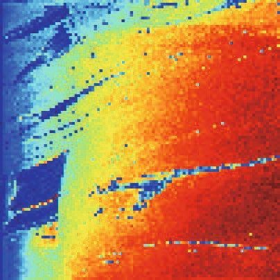
Figure 3. Phase-space maps of normalized coupling predictive causation via correlation, mutual information,
CCM and OIF for varying true causal interactions. Both true causal interactions βxy and βyx are free varying
within the range [0, 1], indicating a bivariate model S(βxy,βyx ) where both species (or variables more generally)
are interacting with each other with different strength. (A) normalized correlation coefficient, (B) normalized
mutual information, (C) and (E) normalized CCM correlation coefficient (ρ) for interaction directions of
X → Y and Y → X , (D) and (F) normalized transfer entropy (TE) from OIF model for interaction directions of
X → Y and Y → X .
of cooperative and uncooperative interactions can result into net interactions at the ecosystem scale manifesting
neutral patterns, or net interactions may lead to niche patterns biased toward strong environmental or biological
factors52. Certainly, cooperation in a biological sense should be interpreted on a case by case basis. In a broader
Scientific Reports | (2021) 11:7094 | https://doi.org/10.1038/s41598-021-86476-9 7
Vol.:(0123456789)www.nature.com/scientificreports/
A 1
0.8
0.6
X(t), Y(t)
0.4
0.2 x
y Blue Green Red
0
0 10 20 30 40 50 0 10 20 30 40 50 0 10 20 30 40 50
t t t
B 1
0.8
0.6
Y(t)
0.4
0.2
0
0 0.2 0.4 0.6 0.8 10 0.2 0.4 0.6 0.8 10 0.2 0.4 0.6 0.8 1
X(t) X(t) X(t)
Figure 4. Dynamics of abundance and predictability for the bidirectional two species ecosystem model. (A)
plots refer to the species abundance in time for the mathematical model in Eq. 1 for different predictability
regimes associated to different interaction dynamics from low to high complexity ecosystem associated to low
and high predictability. Blue, green and red refer to a range of predictable interactions as in Fig. 3: specifically,
Blue is for (βy x , βx y)=(0.18, 0.39) (small mutual interaction, and predominant effect of Y on X), Green is for
(0.64, 0.57) (high mutual interactions, and slightly predominant effect of X on Y), and Red for (0.94, 0.34) (high
mutual interactions, and predominant effect of X on Y). (B) phase-space plots showing the non-time delayed
associations between X and Y corresponding to synchronous and homogeneous, mildly asynchronous and
divergent, and asynchronous and divergent dynamics. The transition from synchronous/small interactions to
asynchronous/high interaction leads to a transition from modular to nested ecosystem interactions when more
than one species exist (Fig. 6).
uncertainty propagation perspective49, “cooperation” between variables means that variables contribute similarly
to the uncertainty propagation, while “competition” means that one variable is predominant over the other in
terms of magnitude of effects since TE is proportional to the magnitude rather than the frequency of effects. For
the former case the total entropy of the system is higher than the latter case. Interestingly, correlation corr (β), ρ
and TE show similar patterns in both organization and value range (but not in singular values of course), which
sheds some important conclusions about the similarity and divergence of these methods as well as their capacity
and limitations in characterizing non-linear systems.
When comparing the phase-space patterns from CCM and OIF (displaying ρ and TE) a more colorful and
informative pattern is revealed by OIF. This means that TE gives a better gradient when tracking the increasing
strength of causality for increasing values of βxy and βyx . When comparing the phase-space patterns for the two
causal directions of “X → Y ′′ and “Y → X ′′ , phase-space maps from CCM are very similar, while those from
TE present apparent differences in the strength of effects for the two opposite direction of interaction. Therefore,
OIF is more sensitive to the direction of interaction compared to CCM when detecting directional causality.
These results imply that TE performs better to distinguish directional embedded physical interactions (that
are dependent on direct interactions β-s, species growth rate rx and ry , and contingent values X(t) and Y(t)
determining the total interaction as seen in the model of Eq. (1)) in the species causal relationships. It should
be emphasized how all linear and non-linear interaction indicators are inferring the total interaction and not
only those exerted by β-s. In a broad uncertainty p urview49 the importance of these three factors (β-s, r-s and
X(t)/Y(t)) depends on their values and probability distributions that define the dynamics of the system; dynam-
ics such as defined by the regions identified by patterns in Fig. 3 for the predator-prey system in Eq. (1). In
principle, the higher the difference between these three interaction factors in the species considered, the higher
the predictability and sensitivity of OIF. Figure 4 highlights three different dynamics corresponding to the TE
blue, green and red regions in Fig. 3.
In all dynamical states represented by Fig. 3, species are interacting with different magnitudes and this defines
distinct network topologies. Three prototypical dynamics are shown in Fig. 4 with colors representative of ρ
and TE in Fig. 3. The “blue” deterministic dynamics has very high synchronicity and no divergence considering
Scientific Reports | (2021) 11:7094 | https://doi.org/10.1038/s41598-021-86476-9 8
Vol:.(1234567890)www.nature.com/scientificreports/
variable fluctuation range (the gap is deterministic and related to the numerically imposed u = 1), as well as no
linear correlation between non-lagged variables. In perfect synchrony one would have one point in the phase-
space. Thus, absence of correlation does not imply complete decoupling of species but it can be a sign of small
interactions. The “green” dynamics shows a relatively high synchronicity and medium divergence. In the phase-
space of synchronous values of X and Y a correlation is observed with relatively small fluctuations because the
divergence is small. Lastly, the “red” dynamics shows a relatively high asynchronicity and divergence. The sto-
chasticity is higher than previous dynamics and the “mirage correlation” in the phase space has higher variance.
Time-dependent mirage correlations in sign and magnitude mean that correlation (that may suggest common
dynamics in a linear framework) does not imply similarity in dynamics for the two species. Non-linearity is
higher from blue to red dynamics as well as predictability but lower absolute information entropy. Then, it is safe
to say that linear dynamics (or small stochasticity) does not imply higher predictability.
Real‑world sardine–anchovy‑temperature ecosystem. CCM and proposed OIF model are also
used for a real-world fishery ecosystem to infer potential causal interactions between Pacific sardines (Sardinops
sagax) landings, Northern anchovies (Engraulis mordax) and sea-surface temperature (SST) recorded at Scripps
Pier and Newport Pier, California. Sardines and anchovies do not interact physically (or the interaction is low
in number), while both of them are influenced by the external environmental SST that is the external forcing.
To quantify the likely causal interactions between species and SST based on real data, we use CCM considering
the length of time series for convergence of ρ , as well as OIF considering a set of time delays for acquiring stable
values of inferred interactions TEs.
Results from CCM in Fig. 5A (plots from top to bottom) show that no significant interaction can be claimed
between sardines and anchovies, as well as from sardines or anchovies in the SST manifold which expectedly
indicates that neither sardines nor anchovies affect SST. This latter results, considering its biological plausibility
should be taken as one validation criteria of predictive models, or complimentary as a test for anomaly detec-
tion of spurious interactions. The reverse effect of SST on sardines and anchovies can be quantitatively detected
with the correlation coefficient ρ as well as TE. Although the calculated causations between SST and sardines or
anchovies are moderate, CCM is able to provide a good performance in causality inference when the length of
time series used is long enough due to convergence requirement.
Figure 5B shows OIF’s results of inferred causal interactions between sardines, anchovies and SST dependent
on the time delay u. For sardines and anchovies, OIF exposes bidirectional interactions that are actually biologi-
cally plausible, especially when both populations coexist in the same habitat, versus the results of CCM that
infer ρ = 0. Ecologically speaking, even though fish populations do not directly influence sea temperature, we
can find some clues about SST in fish populations influenced by SST. These clues can be interpreted as informa-
tion of SST encoded in fish populations over abundance time records. So, observations of fish populations can
be used to inversely predict the change of SST; this can be interpreted as “reverse predictability” (or “biological
hindcasting”) in a similar way of when predicting historical climate change from ice cores. This information is
captured by OIF, leading to nonzero values of TE from fish populations to SST. In this regard, we emphasize the
distinction between direct and indirect (reverse) information flow, where direct information flow is most of the
time larger and signifies causality (e.g. of SST for sardine and anchovies), and indirect (reverse) information
flow that is typically smaller and signifies predictability (e.g. sardine and anchovies for ocean fluctuations). It is
possible—especially for linear systems where an effect is observed immediately after a change—that information
of SST encoded in fish populations is high if the interdependence, represented by the functional time delay u, of
the environment-biota is small. However, for highly non-linear systems such as fishes and the ocean, changes in
temperature may take a while before being encoded into fish population abundance53. Thus, it is correct that the
highest values of TE are for high u. Values of TE for small u-s are numerical artifacts related to systematic errors
leading to overestimation of interactions that are time-delayed eventually. One way to circumvent this problem,
largely present for short time series, would be to extend time series by conserving their dynamics (see Li and
Convertino39) or to bound the calculation of TE only for the u that maximizes the Mutual Information; this
would provide an average u within a range where TE is approximately invariant. Thus, for the effect of external
SST on sardines and anchovies, OIF model gives unstable causal interactions with bias for lower time delays due
to known dependencies of TE on u (such as cross-correlation for instance) that establishes the temporal lag on
which the dependency between X and Y is evaluated. In a sense, plots in Fig. 5B are like cross-variograms for the
pairs of variables considered. TE becomes stable when the time delay is located in an appropriate range. It means
that OIF requires an optimal time delay that makes results of the causality inference robust and that is related
to optimal TEs (as highlighted in Li and Convertino39 and Servadio and Convertino49) that defines the most
likely interdependency between variables for the u with the highest predictability. The fact that TE of sardine and
anchovies to SST is high for same small ranges of u may be also a byproduct of data sampling, i.e., fish and SST
sampling locations are different (fish abundance is actually about fish landings) and that can introduce spurious
correlations/causation. Overall, these findings suggest that the OIF model provides more plausible results, but
it requires careful selection of optimal time delays.
Figure S1 shows the relationships between normalized ρ and TE estimated for all selected values of L and u
of pairs in Fig. 5 (sardine-anchovy, sardine and SST, anchovy and SST). These plots show opposite results than
the proportionality between ρ and TE in Fig. 3 because non-optimal values are used, that is non-convergent ρ -s
and suboptimal TE during the interaction inference procedure (Fig. S1). TE for too small u-s determines over-
estimation of interactions due to the implicit assumptions that variables have an immediate effect on each other
and that is not always the case as highlighted by the vast time-lagged determined non-linear regions in Fig. 3. If
“transitory” values of ρ for small L are disregarded, as well as TEs for small u-s, the relationship between ρ and
TE shows a correct linear proportionality.
Scientific Reports | (2021) 11:7094 | https://doi.org/10.1038/s41598-021-86476-9 9
Vol.:(0123456789)www.nature.com/scientificreports/
A B
0.0 0.2 0.4 0.6 0.8 1.0
0.0 0.2 0.4 0.6 0.8 1.0
Anchovy to Sardine
Sardine to Anchovy
TE
ρ
10 20 30 40 50 60 70 80 5 10 15 20
0.0 0.2 0.4 0.6 0.8 1.0
0.0 0.2 0.4 0.6 0.8 1.0
SST to Sardine
Sardine to SST
TE
ρ
10 20 30 40 50 60 70 80 5 10 15 20
0.0 0.2 0.4 0.6 0.8 1.0
0.0 0.2 0.4 0.6 0.8 1.0
SST to Anchovy
Anchovy to SST
TE
ρ
10 20 30 40 50 60 70 80 5 10 15 20
L Time delay (u)
Figure 5. Inferred predictive causality for the sardine-anchovy-Sea Surface Temperature ecosystem. CCM
correlation coefficient (ρ) and OIF predictor (TE) are shown in the left and middle plots for different pairs
considered (sardine–anchovy, sardine and SST, anchovy and SST from top to bottom).
Real‑world multispecies ecosystem. Interactions between fish species living in the Maizuru bay are
intimately related to external environmental factors of the ecosystem where they live, the number of species
living in this region considering also the unreported ones and biological species interactions, which lead to a
complex dynamical nonlinear system. In Fig. 6 the network of observed fish species (Table S1) is reported where
only the interactions considered in Ushio et al.37 for the CCM are reported. This is because the goal is to compare
the CCM inferred network to the TE-based one based on abundance. Figure 7 shows the temporal fluctuations
of abundance and the functional interaction matrices of ρ and TE. In this paper we study and compare aver-
age ecosystem networks for the whole time period considered but dynamical networks can also be extracted
via time-fluctuating ρ and TE as shown in Fig. S3. These dynamical networks can be useful for studying how
diversity is changing over time and ecosystem stability (Figs. S4, S6–S7) as well as understanding the relation-
ship between ρ and TE (Fig. S5). In the network of Fig. 6 the color and width of links are proportional to the
magnitude of TE (Table S2); for the former a red-blue scale is adopted where the red/blue is for the highest/
lowest TEs. The diameter is proportional to the Shannon entropy of the species abundance pdf (Table S3). The
color of nodes is proportional to the structural node degree, i.e. how many species are interconnected to others.
Therefore, the network in Fig. 6 is focusing on uncooperative species whose divergence and/or asynchronicity
(that is a predominant factor in determining TE over divergence) is large. Yet, the connected species are rarely
but strongly interacting in magnitude rather than frequently and weakly (i.e., cooperative or similar dynamics).
Additionally, the species with the smallest variance in abundance are characterized by the smallest Shannon
entropy (smallest nodes) and more power-law distribution although the latter is not a stringent requirement
since both pdf shape and abundance range (in particular maximum abundance) play a role in the magnitude
of entropy. Average entropy such as average abundance are quantities with limited utility in understanding the
dynamics of an ecosystem as well as ecological function. Nonetheless, species with high average abundance (e.g.
Scientific Reports | (2021) 11:7094 | https://doi.org/10.1038/s41598-021-86476-9 10
Vol:.(1234567890)www.nature.com/scientificreports/
1
2
15
3
14
4
13
5
12
6
11
7
10
9 8
Figure 6. Part of the estimated species interaction network for the Maizuru Bay ecosystem. Species properties
are reported in Table S1. The color and width of links are proportional to the magnitude of TE (Table S2); for the
former a red-blue scale is adopted where the red/blue is for the highest/lowest TEs. The diameter is proportional
to the Shannon entropy of the species abundance (Table S3) that is directly proportional to the degree of
uniformity of the abundance pdf and the diversity of abundance values (e.g., the higher the zero abundance
instances the lower the entropy). The color of nodes is proportional to the structural node degree, i.e. how many
species are interconnected to others after considering only the CCM derived largest interactions (see Ushio
et al.37 and Fig. 7). Other interactions exist between species as reported in Fig. 7. TE is on average proportional
to ρ (Figs. S4 and S5). Freely available fish images are from FishBase https://www.fishbase.in/search.php; the
network was created in Matlab and the composition of network and images was made in Adobe Illustrator
version 21 (2017) https://www.adobe.com/products/illustrator.html.
species 5) have a very regular seasonal oscillations and the largest number of interactions with divergent spe-
cies. This dynamics is expected considering the population size of these dominant species and their synchrony
with regular environmental fluctuations.
Figure S2 shows that the strongest linear correlation is for the most divergent and asynchronous species (from
species 4–9) for which both ρ and TE are the highest (Fig. 7B,C). This confirms the results of Fig. 3 and the fact
that competition (or dynamical diversity more generally) increases predictability. This also highlights the fact
that linear correlation among state variables does not imply synchronicity or dynamic similarity as commonly
assumed. The interaction matrices in Fig. 7B, C confirm that TE has the ability to infer a larger gradient of inter-
actions than ρ and the total entropy of the TE matrix is lower than ρ . Pairwise the inferred interaction values
by CCM and OIF are different but ρ and TE patterns appear clearly similar and yet proportional to each other.
CCM and OIF models are applied to calculate the potential interactions between all pairs of species. Fig-
ure 7B,C show interaction matrices describing the normalized ρ from CCM and TE from OIF model of all
pairwise species, respectively. The greater the strength of likely interaction, the warmer the color. These results
demonstrate that CCM and OIF model present similar patterns for the interaction matrices in terms of interac-
tion distribution, gradient and magnitude in order of similarity. This indicates that both CCM and OIF are able
to infer the potentially causal relationships between species. Compared to the CCM interaction heatmap the
OIF heatmap presents larger gradients of inferred interactions that highlight the divergence and asynchrony in
fish populations of species 4–9 from other species. This difference can be observed in Figure S2 that shows the
strongest linear correlations for the most divergent and asynchronous species (4–9). It is worth noting that spe-
cies 4-8 are all native species (See Table SS11). Therefore, despite the patterns of interactions of CCM and TE are
Scientific Reports | (2021) 11:7094 | https://doi.org/10.1038/s41598-021-86476-9 11
Vol.:(0123456789)www.nature.com/scientificreports/
1.Aurelia aurita
2.Engraulis japonicus
A 3.Plotosus lineatus japonicus
4.Sebastes inermis
5.Trachurus japonicus
5000 6.Girella punctata
7.Pseudolabrus sieboldi
4000 8.Halichoeres poecilopterus
9.Halichoeres tenuispinnis
Abundance
10.Chaenogobius gulosus
3000 11.Pterogobius zonoleucus
12.Tridentiger trigonocephalus
13.Siganus fuscescens
2000
14.Sphyraena pinguis
15.Rudarius ercodes
1000
0
15
10 2016
2014
2012
5 2010
Species NO. 2008
2006
2004
0 2002 Year
B ρ/max(ρ) C TE/max(TE)
15
14
13
12
11
10
Species
9
8
7
6
5
4
1.00
3 0.75
2 0.50
0.25
1 0.00
1 2 3 4 5 6 7 8 9 10 11 12 13 14 15 1 2 3 4 5 6 7 8 9 10 11 12 13 14 15
Species Species
Figure 7. Normalized species interactions matrices inferred by CCM and OIF models for Maizuru Bay
ecosystem. In the census of the aquatic community, 15 fish species were counted in total. Interaction
inferential models use time lagged abundance magnitude (CCM) or pdfs of abundance (OIF) shown in (A).
(B) normalized CCM correlation coefficients (ρ) between all possible pairs of species. (C) normalized transfer
entropies (TEs) between all pairs of species from the OIF model. Both CCM and OIF predict that the most
interacting species (in terms of magnitude rather than frequency) are 7, 8 and 9 on average. Thus, interaction
matrices are more proportional to the asynchronicity than the divergence of species in terms of abundance pdf,
although abundance value range defines the uncertainty (and diversity) for each species that ultimately affects
entropy and interactions (e.g., if one species have many zero abundance instances or many equivalent values,
such as species 2, TEs of that species are expected to be low due to lower uncertainty despite the asynchrony and
divergence).
similar, CCM allows one a better identification of clusters of species with similar or distinct interaction ranges.
Additionally TE estimates some weak observed interactions such as of species 2 (E. japonicus) with others, while
CCM essentially considers null interactions for these species.
Scientific Reports | (2021) 11:7094 | https://doi.org/10.1038/s41598-021-86476-9 12
Vol:.(1234567890)You can also read