R 1337 - A liquidity risk early warning indicator for Italian banks: a machine learning approach - Temi di discussione

Temi di discussione
 (Working Papers)

 A liquidity risk early warning indicator for Italian banks:
 a machine learning approach

 by Maria Ludovica Drudi and Stefano Nobili
June 2021

 1337
 Number

Temi di discussione
(Working Papers)

A liquidity risk early warning indicator for Italian banks:
a machine learning approach

by Maria Ludovica Drudi and Stefano Nobili

Number 1337 - June 2021

The papers published in the Temi di discussione series describe preliminary results and
are made available to the public to encourage discussion and elicit comments.
The views expressed in the articles are those of the authors and do not involve the
responsibility of the Bank.

Editorial Board: Federico Cingano, Marianna Riggi, Monica Andini, Audinga
Baltrunaite, Marco Bottone, Davide Delle Monache, Sara Formai, Francesco
Franceschi, Adriana Grasso, Salvatore Lo Bello, Juho Taneli Makinen, Luca
Metelli, Marco Savegnago.
Editorial Assistants: Alessandra Giammarco, Roberto Marano.

ISSN 1594-7939 (print)
ISSN 2281-3950 (online)
Printed by the Printing and Publishing Division of the Bank of Italy

A LIQUIDITY RISK EARLY WARNING INDICATOR FOR ITALIAN BANKS:
 A MACHINE LEARNING APPROACH

 by Maria Ludovica Drudi† and Stefano Nobili‡

 Abstract
 The paper develops an early warning system to identify banks that could face liquidity
crises. To obtain a robust system for measuring banks’ liquidity vulnerabilities, we compare
the predictive performance of three models – logistic LASSO, random forest and Extreme
Gradient Boosting – and of their combination. Using a comprehensive dataset of liquidity
crisis events between December 2014 and January 2020, our early warning models’ signals
are calibrated according to the policymaker's preferences between type I and II errors. Unlike
most of the literature, which focuses on default risk and typically proposes a forecast horizon
ranging from 4 to 6 quarters, we analyse liquidity risk and we consider a 3-month forecast
horizon. The key finding is that combining different estimation procedures improves model
performance and yields accurate out-of-sample predictions. The results show that the
combined models achieve an extremely low percentage of false negatives, lower than the
values usually reported in the literature, while at the same time limiting the number of false
positives.

JEL Classification: C52, C53, G21, E58.
Keywords: banking crisis, early warning models, liquidity risk, lender of last resort, machine
learning.
DOI: 10.32057/0.TD.2021.1337

 Contents

1. Introduction ........................................................................................................................... 5
2. Data and variables ............................................................................................................... 10
3. A policymaker’s loss function and the usefulness measure ................................................ 18
4. The classification models .................................................................................................... 21
 4.1 Logistic LASSO ........................................................................................................... 22
 4.2 Random forest .............................................................................................................. 24
 4.3 Extreme Gradient Boosting .......................................................................................... 26
5. Results and model combination........................................................................................... 27
6. Robustness checks ............................................................................................................... 33
7. Conclusion ........................................................................................................................... 37
References ................................................................................................................................ 40
Figures and tables ..................................................................................................................... 45

_______________________________________
†
 Bank of Italy, Directorate General for Economics, Statistics and Research.
‡
 Bank of Italy, Directorate General for Markets and Payment Systems.

1. Introduction1

The main economic function performed by a bank is intermediation, i.e. the transfer of
financial resources from those who have them to those who instead lack them. This
activity takes place through the transformation of maturities: banks collect short-term or
demand liabilities (deposits) from the public and transform them into less liquid assets by
financing projects over longer time horizons and exposing themselves to liquidity risk.
This liquidity and maturity transformation can create an incentive for investors to
withdraw quickly funds in adverse situations. Creditors’ loss of confidence towards a
bank can trigger a liquidity crisis (Diamond and Dybvig, 1983), which could also cause
difficulties to other financial institutions, threatening the overall stability of the system
and adversely affecting the economy. Historians and economists often refer to widespread
creditor and investor runs as “financial panics”.

To deal with the effects of these structural weaknesses and prevent contagion risks in a
particularly strategic sector such as the credit sector, central banks can intervene as a
lender of last resort (LOLR). Providing Emergency Liquidity Assistance (ELA)
represents the most traditional tool to contrast financial instability resulting from a
liquidity crisis (BIS CGFS Papers, 2017; Dobler et al., 2016). ELA to financial
institutions is a core responsibility of central banks because of their unique ability to
create liquid assets in the form of central bank reserves, their central position within the
payment system and their macroeconomic stabilization objective. The global financial
crisis served as a reminder of the critical importance of the LOLR function in restoring
financial stability. The provision of ELA by the central bank should only be considered
when other funding solutions have already been fully explored, but it represents a process
that may have to happen very fast. To be able to intervene promptly or to adopt pre-
emptive actions, central banks must have a set of methodological tools useful to anticipate
the occurrence of these situations of instability. These tools are useful to attempt
anticipating the need for liquidity support in advance before formal action is required, so

1
 Any views expressed in this paper are the authors’ and do not necessarily represent those of the Bank
 of Italy. We thank Luigi Cannari, Patrizia Ceccacci, Sara Cecchetti, Gioia Cellai, Paolo Del Giovane,
 Taneli Makinen, Franco Panfili, Rosario Romeo, Stefano Siviero, Marco Taboga and two anonymous
 referees for valuable comments and suggestions.

 5

as to enable better information gathering and preparation. After the global financial crisis,
central banks paid particular attention to developing or strengthening their early warning
(EW) models. An EW system pursues the early detection of difficulties in order to start
addressing the problems immediately. According to the literature, it is possible to
distinguish two main strands of EW models. The first regards studies and models at the
micro level designed to signal at an early stage the potential distress of individual
institutions (e.g. Bräuning et al., 2019, Ferriani et al., 2019). The second is based on macro
models attempting to identify the build-up of macro-financial vulnerabilities that threat
the soundness of the banking and financial system as a whole (e.g. Aldasoro et al., 2018,
Alessi and Detken, 2018, Beutel et al, 2018). The latter models are useful to guide
decisions on when to activate macroprudential tools targeting excessive leverage or credit
growth. The present paper focuses on the first strand, applying to Italian banks an EW
system that concentrates on liquidity risk.

The models applied to predicting distress at bank level are usually multivariate systems
that aim to estimate the probability of an institution's distress within a given time horizon
based on a set of input indicators. While not normally providing a fully reliable signal of
any impending weaknesses, these EW systems are particularly useful to highlight those
intermediaries that present greater vulnerabilities, being therefore more exposed to the
risk of entering a crisis. Historically, they have focused on estimating banks’ probabilities
of incurring a crisis starting from the analysis of historical default cases. In these models,
the dependent variable typically assumes the value 1 if a bank is in default in a given
period and 0 otherwise. Input variables are often related to the main intermediaries’ risk
profiles such as capital adequacy, credit, profitability, governance and control systems
and liquidity.

The present paper contributes to the literature on EW models applied to the individual
financial institutions in several ways. First, using the data available to the Bank of Italy,
we shift the focus from the analysis of insolvency risk to liquidity risk introducing a novel
dataset of bank liquidity crisis events, starting from banks that resorted to the central
bank’s ELA.

Unlike most of the literature, which focuses on the analysis of the insolvency risk and
typically proposes a forecast horizon ranging from 4 to 6 quarters, we consider as the

 6

main forecast horizon the 3-month one. This choice depends on the fact that liquidity
crises by their nature tend to arise quickly and require prompt intervention. Indeed, the
choice of the forecast horizon has to satisfy the trade-off between being as short as
possible in order to obtain very accurate estimates and being large enough to allow central
banks to take corrective actions that could possibly avoid the onset of the crisis.

We compare the predictive capabilities of three different models, and then proceed to
combine them. The three models are the logistic LASSO, the random forest and the
Extreme Gradient Boosting. Our results notably improve the predictive performance with
respect to the most usual modeling techniques. To identify the model specification that
optimizes its out-of-sample predictive capacity (Tibshirani, 1996), the first approach uses
a LASSO (Least Absolute Shrinkage and Selection Operator) cross-validation technique,
based on maximizing a binomial logarithmic likelihood function subject to a penalty term.
The second classification method, introduced by Breiman (2001), is a generalization of
decision tree models and computes the estimates by aggregating the forecasts derived
from a large number of different trees. By combining the trees predictions, the variance
of the estimates decreases, making them more efficient2. This phenomenon occurs
because random forest models generate heterogeneity between the different decision
paths by randomly choosing a subset of observations on which the estimate is made
(bagging) and considering only a random subset of indicators at each step (attribute
bagging). Finally, the third method, exactly as the random forest, is a classification model
that generalizes the decision trees models. This time, the trees are combined sequentially
by working on the residuals of the previous tree, thereby reducing estimates bias. The
Extreme Gradient Boosting (XGBoost) algorithm, proposed by Chen and Guestrin
(2016), has become a popular supervised learning algorithm, in particular for financial
time series data. To avoid the overfitting problem, this algorithm uses features
subsampling as the random forest and a regularization parameter to reduce the final
prediction sensitivity to single observations.

2
 Decision trees are extremely sensitive to the specific dataset they are based on. Sometimes they show
 the problem of overfitting: they have a high in sample performance, but are not very versatile if applied
 outside the sample.

 7

The literature on insolvency or liquidity risk of banks usually presents individual models’
results. In contrast, to obtain a more robust system for measuring banks’ liquidity
vulnerabilities, this work follows the approach of comparing and aggregating the
information obtained by the three methods. Indeed, it is likely that different approaches
capture different types of fragility, and therefore can complement each other, giving value
to their simultaneous use (Holopainen and Sarlin, 2017).

Following Sarlin (2013), the models’ signals are calibrated according to the policymaker's
preferences between type I (missing crises) and type II (false alarm) errors modeled by a
loss function. The signals are then aggregated using both a simple average and a weighted
average with a measure of relative usefulness as weight. To take into account central
bank’s preference for models that minimize type I error, in line with bank early warning
literature (e.g. Holopainen and Sarlin, 2017), for each method the loss function has been
optimized attributing a weight to missing a crisis far greater than the one of a false alarm.
The rationale behind this choice follows the fact that an EW signal should trigger actions
by the authority to investigate and possibly restore the liquidity situation of the bank.
Should the analysis reveal that the signal is false, there is no loss of credibility for the
policymaker as model results are not published.

The key finding of the paper is that complementing different estimation procedures
improves model performance and yields accurate out-of-sample predictions of banks’
liquidity crises. Results show that the combined model manages to have an extremely low
percentage of false negatives (missing a crisis) in out-of-sample estimates, equal to 10%,
while at the same time limiting the number of false alarms too. These results are lower
than the values usually reported in the literature. This could depend on our choice to test
the model on a 3-month forecast horizon, which is perfectly suitable for liquidity risk
models, but shorter than the horizon usually considered in insolvency risk models.

This work fits two strands of literature: the first relating to forecasting individual bank
crisis and the second one to optimizing early warning signals through models. An initial
contribution to the first strand is the work of Martin (1977), which uses a logistic
regression based on balance sheet variables (CAMEL rating system: Capital adequacy,
Asset quality, Management quality, Earnings, Liquidity) to predict the default of a set of
US banks between 1970 and 1976. Subsequent literature focused on identifying the

 8

explanatory variables to be included in the model to improve its predictive performance
(Thomson, 1992; Cole and Gunther, 1998; González-Hermosillo, 1999; Jagtiani et al.,
2003; Kraft and Galac, 2007). Other EW models included market indicators, as they are
more responsive in identifying bank’s health status (Flannery 1998; Krainer and Lopez
2003; Campbell et al., 2008). Finally, Poghosyan and Čihák (2011) built an EW system
in which a bank's crisis is identified through a massive search for some keywords in the
press reports.

Works like Kaminsky et al. (1998) have contributed to the second strand of literature.
They introduced the so-called "signal approach" based on the identification of thresholds
beyond which the individual indicators signal a crisis. Demirguc-Kunt and Detragiache
(2000) introduced the use of a loss function that allows the authority to weigh its cost of
missing a crisis (type I error) differently from a false alarm (type II error). Subsequent
works modified the structure of the loss function to adapt it to the specific characteristics
they need (Alessi and Detken, 2011; Lo Duca and Peltonen, 2013; Sarlin, 2013). Lang et
al. (2018) propose a system to derive EW models with an excellent out-of-sample
forecasting performance. The use of a loss function that evaluates the model in terms of
preferences between type I and type II errors is associated with a regularized logistic
regression (logistic LASSO regression) that allows selecting the model specification with
the best forecasting properties.

More recently, the EW literature has started using a wide range of nonparametric
techniques that can be generically traced back to machine learning. Tam and Kiang
(1992), Alam et al. (2000), Boyacioglu et al. (2009), among others, present EW models
based on neural networks, a non-linear approach in which the identification of institutions
facing difficulties is based on some interconnection measures between explanatory
variables. The recent works of Tanaka et al. (2016), Holopainen and Sarlin (2017), Alessi
and Detken (2018) use a random forest to improve the forecasting performance of EW
models. Bräuning et al. (2019) identify cases of individual bank financial distress by
estimating a decision tree model based on the Quinlan C5.0 algorithm.

The remaining part of the paper is organized as follows. Section 2 focuses on data and
variables definition; in Section 3, we present the loss function and a measure of
usefulness. Section 4 describes the classification models. In Section 5, we compare the

 9

results and characteristics of the individual models and we propose two combination
methods. Section 6 describes the results from two robustness checks and Section 7 finally
concludes.

 2. Data and variables

The EW system developed in this paper uses Bank of Italy’s confidential data on recourse
to ELA as well as supervisory reporting and market data, covering all banks that operate
in Italy over a period of more than 5 years, from December 2014 to January 2020. The
sources of bank-level data are the Common Reporting (COREP, containing capital
adequacy and risk-specific information), the Financial Reporting (FINREP, which
includes balance sheet items and detailed breakdowns of assets and liabilities by product
and counterparty), both available since December 2014, and other datasets from national
supervisory reporting3.

The EW model estimation is based on the interaction between a set of attributes, selected
from those that can better signal the onset of potential crises, and a binary target variable
that takes value 1 if a bank is going through a period of crisis and 0 otherwise. To
construct this binary variable it is necessary to identify which banks are facing a crisis.
To the best of our knowledge, we adopt an innovative perspective with respect to the
prevailing literature. Indeed, we focus on the analysis of liquidity risk identifying the
period in which the liquidity distress starts, builds up and possibly outbreaks. This choice
helps to detect cases of financial difficulties early enough to allow for a timely
intervention of the authorities (see e.g. Rosa and Gartner, 2018 and Bräuning et al., 2019).

In order to have an EW system on bank liquidity crises, we defined our target variable in
an extensive way. First, we considered banks that resorted to the central bank’s ELA.
Central banks may provide ELA when solvent financial institutions face temporary
liquidity shortages and after other market and/or private funding sources have been
exhausted. ELA aims at mitigating sudden funding pressures that could, if not addressed,
jeopardize financial stability. By providing liquidity support on a temporary basis, central

3
 These variables come from banks’ balance sheet data at the highest degree of consolidation. To get the
 monthly equivalent for variables available only on a quarterly basis, we kept the last value constant.

 10

banks seek to prevent a systemic loss of confidence that can spread to otherwise healthy
institutions. The Bank of Italy (BoI) provides ELA under the European System of Central
Banks (ESCB) ELA Agreement, published by the European Central Bank (ECB) in May
2017, which places the ELA function within the prerogatives of National Central Banks.
In BoI, the function to provide ELA is allocated to the competent organizational unit
within the Markets and Payment Systems Directorate.

Considering only banks’ recourse to ELA, however, would be too narrow as ELA is only
one of the possible outcome of a liquidity crisis. Moreover, banks’ recourse to ELA in
Italy has not been frequent. For this reason, we extended the definition of liquidity crises
to include other possible manifestations of banks’ liquidity deterioration. Among other
situations that arguably indicate a state of liquidity distress, we considered banks subject
to restrictive measures on participation to monetary policy operations. Indeed, according
to the General Documentation (Guideline 2015/510 of the ECB and following
amendments)4, the Eurosystem allows the participation to monetary policy operations
only to financially sound institutions. If this condition is not respected at a certain point
in time or there are instances that are deemed to affect negatively the financial soundness
of the bank, the Eurosystem can limit, suspend or exclude it from monetary policy
operations. These measures typically follow a reduction of capital ratios under the
minimum regulatory requirements; but even if they are conceptually closer to solvency
than illiquidity risk (though, of course, telling the two apart is difficult) they usually have
immediate negative consequences on the bank’s liquidity position.

In addition, to promptly identify liquidity distress events, we took into account banks
subject to enhanced monitoring by the BoI’s Supervisory Directorate and brought to the
attention of the BoI’s Markets and Payment Systems Directorate, regardless of whether
or not the bank was eventually given access to ELA. Indeed, the Supervisory Department
puts banks under enhanced monitoring when liquidity is starting to deteriorate and the
frequency of regular supervisory liquidity reporting is deemed insufficient to adequately
monitor emerging liquidity strains.

4
 https://www.ecb.europa.eu/ecb/legal/pdf/oj_jol_2015_091_r_0002_en_txt.pdf

 11

We also included banks that received State support either in the form of Government
Guaranteed Banks Bonds (GGBBs) or in the form of a precautionary recapitalization5.

Moreover, we considered banks under early intervention measures as defined by the
BRRD6, e.g. banks placed under special administration and/or subject to the appointment
of a temporary administrator, regardless of the fact that special or temporary
administration succeed in rehabilitating the bank. Although not all banks in the sample
were placed under early intervention measures due to liquidity problems, all these events
are connected directly or indirectly to a liquidity deterioration. Indeed, even if the aim of
early intervention measures is restoring ailing institutions in the medium time horizon, in
the short time it could produce a negative effect on the liquidity situation, due to deposit
withdrawals by the customers. This assumption is confirmed by performing a panel fixed
effect regression where the independent variable is a dummy that takes value 1 if the bank
in that month was placed under early intervention measures and 0 otherwise and the
dependent variable is the monthly change of the sight deposit variation (Table A1). In this
way, we are able to capture changes in the deposit trend due to early intervention. In line
with our expectations, the coefficient is negative and statistically significant.

5
 Art. 32, point 4, letter d of the BRRD: “[…] the extraordinary public financial support takes any of the
 following forms: i) a State guarantee to back liquidity facilities provided by central banks according to
 the central banks’ conditions; ii) a State guarantee of newly issued liabilities; iii) an injection of own
 funds or purchase of capital instruments at prices and on terms that do not confer an advantage upon the
 institution […].
6
 The early intervention measures are set in Artt. 27 - 29 of the BRRD. Art. 27: “Where an institution
 infringes or, due, inter alia, to a rapidly deteriorating financial condition, including deteriorating
 liquidity situation, […] is likely in the near future to infringe the requirements of Regulation (EU) No
 575/2013, Directive 2013/36/EU, Title II of Directive 2014/65/EU or any of Articles 3 to 7, 14 to 17,
 and 24, 25 and 26 of Regulation (EU) No 600/2014, Member States shall ensure that competent
 authorities have at their disposal […] at least the following measures: a) require the management body
 of the institution to implement one or more of the arrangements or measures set out in the recovery plan
 […]; b) require the management body of the institution to examine the situation, identify
 measures to overcome any problems identified and draw up an action program to overcome those
 problems […]; c) require the management body of the institution to convene […]; d) require one or
 more members of the management body or senior management to be removed or replaced […]; e)
 require the management body of the institution to draw up a plan for negotiation on restructuring
 of debt […]; f) require changes to the institution’s business strategy; g) require changes to the legal or
 operational structures of the institution; h) acquire, including through on-site inspections and provide
 to the resolution authority, all the information necessary in order to update the resolution plan and
 prepare for the possible resolution of the institution […].” Art. 28 “Removal of senior management and
 management body”, Art. 29 “Temporary administrator”.

 12

Finally, if not already detected, we included banks deemed to be failing or likely to fail
(FOLTF) for liquidity reasons7.

Usually a bank in liquidity crisis sequentially experiences various events of liquidity
distress. Given the importance of the time dimension for a model aiming to predict a
crisis, we considered the beginning of the crisis from the starting date, if available, of the
first liquidity distress event. Indeed, the full-blown crisis event is often preceded by a
period in which the bank's liquidity position gradually deteriorates, although each
situation is different from the others. In some cases, it is possible to identify precisely the
triggering event, other times the cause is more remote and it is not easy to define an
unequivocal starting point. To improve the accuracy in identifying crisis periods, we
carried out an analysis on the CDS and bonds (senior and subordinated) market trends, as
their dynamics usually anticipate the evolution of the issuer's health8. The model is run
on a monthly basis. In line with the majority of the EW literature, institutions that enter
in liquidity distress are recorded as stressed banks as long as the crisis is ongoing (the
target variable takes value 1), while at the end of that period they are changed back to
their original value of 0. This choice depends on the fact that we are interested in
understanding the dynamics of banks entering and exiting the distress status.

Following these criteria, during the analysed period (December 2014 - January 2020), we
identified 31 banks that have gone through periods of liquidity crisis of different lengths,
for a total of 527 out of 12,761 observations. The crisis events show a peak during 2016,
reaching a maximum of 6.2% of the total number of observations in the year (Figure A1).

To check the robustness of our results, we considered two further specifications of the
target variable. The first one is based on a more restrictive definition of liquidity events.
We considered only the events more closely linked to a liquidity deterioration such as
resorting to central bank’s ELA, benefiting from State support through Government

7
 The FOLTF for liquidity reasons is set in Art. 32 of the BRRD. Art.32, point 4 “[…] an institution shall
 be deemed to be failing or likely to fail in one or more of the following circumstances: […]
 (c) the institution is or there are objective elements to support a determination that the institution
 will, in the near future, be unable to pay its debts or other liabilities as they fall due. […]”.
 So far, no Italian bank has been declared FOLTF for liquidity reasons.
8
 For intermediaries for which such data are available, the onset of the crisis has been made to coincide
 with increases in premiums and / or returns higher than the 90th percentile of the historical distribution.

 13

Guaranteed Banks Bonds (GGBBs) or, finally, being subject to enhanced liquidity
monitoring by the BoI’s Supervisory Directorate and brought to the attention of the BoI’s
Markets and Payment Systems Directorate. Following these criteria, we identified 15
banks that have gone through periods of liquidity crisis of different lengths, for a total of
376 out of 12,761 observations.

In the second robustness check, we considered as liquidity crisis event only the first month
in which one of the events previously described occurred and excluded from the dataset
the following observations related to that event for that bank. However, we allow for the
possibility that during the period a bank incurs in different liquidity crises. We identified
39 observations associated to a liquidity crisis event. In this setting, given the limited
occurrence of crisis events (0.3%), we oversampled the minority class by simply
duplicating examples from that class in the training dataset prior to fitting the model (e.g.
Chawla et al., 2002).

Early-warning models aim at signalling crisis events in advance, but the specific forecast
horizon will depend on the application at hand. We considered as the main forecast
horizon for our analyses the 3-month one, a time span that would give the authorities
enough time to adopt pre-emptive actions. This choice depends on the fact that liquidity
crises by their nature tend to quickly build-up and require prompt intervention. Indeed,
the choice of the forecast horizon has to satisfy the trade-off between being as short as
possible in order to obtain very accurate estimates and being large enough to allow central
banks to take corrective actions that could possibly avoid the onset of the crisis.

As attributes, we considered 20 indicators selected in order to capture the peculiarities of
the financing structure of Italian banks.

The indicator that best provides a first measure of banks’ liquidity is the Liquidity
Coverage Ratio (LCR). The LCR is a coverage index that aims at ensuring that an
intermediary maintains an adequate stock of freely available high quality liquid assets
(HQLA) to meet any liquidity needs over 30 days in a stressful scenario. It is computed
according to the following formula:

 =
 − min⁡( ; ⁡75%⁡ )

 14

where outflows are calculated by multiplying the outstanding balances of various
categories or types of liabilities and off-balance sheet commitments by the rates at which
they are expected to run off or be drawn down in a specified stress scenario. Inflows are
calculated by multiplying the outstanding balances of various categories of contractual
receivables by the rates at which they are expected to flow in under the scenario up to an
aggregate cap of 75% of outflows. The LCR has been a regulatory requirement since
October 2015 and starting from 1st January 2018 the lowest allowed value is 100%.

The asset encumbrance ratio (AE) and the asset encumbrance eligible ratio (AEE) both
provide a measure of the share of assets tied up in financing transactions, but the second
one considers only the subset of assets eligible for monetary policy operations. The
eligibility requirement represents an approximation of the marketability of an asset;
therefore, the AEE index measures the encumbered portion of the most easily tradable
assets. They can be computed according to the following formulas:

 ⁡ + ⁡ ⁡ ⁡ 
 =
 ⁡ + ⁡ ⁡ 

 ⁡ ⁡ + ⁡ ⁡ ⁡ ⁡ 
 =
 ⁡ ⁡ + ⁡ ⁡ ⁡ 

From the liquidity risk point of view, the analysis of the encumbrance is important since
the scarce availability of unencumbered collateral means that the bank has lower
financing capacity in stressful situations. In addition, high and increasing AE levels, to
the extent that they represent an element of fragility of the intermediary, could lead to
greater difficulties in placing unsecured financing instruments on the market.

Then, we consider two variables related to sight deposits: their variation and a coverage
index. The first one is a weighted average of the deposits monthly changes during the
previous 12 months, with a greater weight ( ) for the most recent data.

 11

 ℎ ⁡ ⁡ ℎ = ∑ ⁡∑ Δ⁡ ℎ ⁡ − ∗ 
 =1 =0

 = , = 0.9⁡

 15

This allows to capture their temporal evolution and, therefore, to have information about
the depositors' confidence level toward a bank.

On the other hand, the second indicator is computed as the difference between cash and /
or easily disposable assets9 and bonds maturing within the year over total sight deposits.

 ⁡ ⁡ − ⁡ 
 ℎ ⁡ ⁡ ⁡ ⁡ ⁡ = ⁡
 ℎ ⁡ 

 ⁡ = ⁡ + ⁡ 
 + ⁡ ⁡ 

The indicator provides a measure of the bank's ability to cope with a reduction in sight
deposits through its cash and cash equivalents, under the assumption that it is unable to
renew the bonds falling due within the year.

Starting from the components of this latter indicator, we built two other attributes. The
first one is the ratio between our measure of liquid assets and bank’s total assets, while
the second one is the ratio between liquid assets and sight deposits, without considering
the maturing bonds.

The Eurosystem dependency index is the ratio between the share of Eurosystem
refinancing to total funding and a level of capitalization, measured by the CET1 ratio:

 ⁡ 
 ⁡ ⁡ = ⁡
 ⁡ ∗ 1

The inclusion of the capital ratio allows discriminating banks that resort to monetary
policy operations to optimize their financing cost from those that, instead, resort to it
because they have difficulties in accessing the market. To be thorough, we also included
in the models the ratio of Eurosystem refinancing over total funding and the ratio of
Eurosystem refinancing over total assets.

9
 The easily disposable assets are composed of liquidity deposited in the current accounts with the Bank
 of Italy in excess with respect to the minimum reserve requirement (excess liquidity),
 overcollateralization in the monetary policy collateral pool and uncommitted eligible securities outside
 the collateral pool.

 16

The fragility index on the bond market is computed as the difference between net issues10
and bonds falling due in the following 12 months, where both measures are reported on a
monthly base, over total outstanding bonds:

 ⁡ − ⁡ 
 ⁡ ⁡ ⁡ ℎ ⁡ ⁡ ⁡ = ⁡
 ⁡ ⁡ ⁡ 

This indicator is included as it allows comparing the ability to renew bond financing with
the degree of reliance on this source of funding.

With reference to the bond market, we also computed two other attributes: the ratio
between net issues and total outstanding bonds and the ratio between bonds falling due in
the following 12 months and total outstanding bonds.

The Net Cash Outflows (NCO) over total assets indicator, comparing the LCR
denominator with total assets, allows to analyze the liquidity risk from a complementary
perspective with respect to the one of the LCR and to obtain a relative measure of the net
outflows in a 30-day horizon.

 ⁡ ℎ⁡ 
 ⁡ ℎ⁡ ⁡ ⁡ ⁡ ⁡ = ⁡
 ⁡ ⁡ 

Then, we included the capital ratios (CET1, Tier1 and Total Capital Ratio) and the NPL
ratio as their deterioration usually involves a worsening of an institution liquidity
situation. Furthermore, based on the rules set out in the Eurosystem's General
Documentation, a failure to comply with capital requirements, undermining banks’
solvency, could result in the limitation of the existing refinancing or in the suspension
from monetary policy operations with potential consequences on banks liquidity position.

Finally, we considered two variables related to the overall system: the indicator of
systemic liquidity risk in the Italian financial markets proposed by Iachini and Nobili
(2014), and the 10-year BTP yield. The former is a coincident indicator of systemic
liquidity risk that exploit standard portfolio theory to take account of the systemic
dimension of liquidity stress in the financial market. Three sub-indices reflecting liquidity

10
 Net issues are monthly equivalent values of quarterly data moving averages.

 17

stress in specific market segments (the money market, the secondary market for
government securities, and the stock and corporate bond markets) are aggregated in the
systemic liquidity risk indicator in the same way as individual risks are combined in order
to quantify the overall portfolio risk. The aggregation takes into account the time-
varying cross-correlations between the sub-indices, using a multivariate GARCH
approach. This is able to capture abrupt changes in the correlations and makes it possible
for the indicator to identify systemic liquidity events precisely. The inclusion of the 10-
year BTP yield aims at controlling for the interconnection between financial health of
banks and of sovereigns, the so-called sovereign-bank nexus. Indeed, a souring of the
sovereign funding conditions might cause an increase in banks’ risk. These two variables
are useful to classify the effect on single bank’s liquidity vulnerability stemming from the
overall Italian financial market.

Tables A2, A3 and A4 show respectively some descriptive statistics for each of these
indicators and their correlation matrices, both non-standardized and standardized
(through a transformation based on their empirical cumulative distribution function, CDF,
involving the computation of order statistics11). From the analysis of the correlation
matrices, it appears evident that our indicators are constructed to focus on specific and
different aspects of funding liquidity risk thereby showing low correlation. In line with
expectations, the LCR is negatively correlated with all the variables based on Eurosystem
refinancing. Besides, AER and AEER are correlated among each other and with the
Eurosystem dependency index. Finally, the correlations between capital ratios are strong.

 3. A policymaker's loss function and the usefulness measure

Early warning models typically forecast crisis probabilities; by combining them with
thresholds based on policymaker's preferences, they produce binary signals (in this
framework liquidity crisis/no liquidity crisis). Converting probabilities into clear signals

11
 We prefer the CDF approach to “classic” standardization (i.e. by subtracting the sample mean from the
 raw indicator and dividing this difference by the sample standard deviation). Classic standardization, in
 fact, implicitly assumes variables to be normally distributed; but since many indicators violate this
 assumption, the risk that the results obtained from the use of standardized variables are sensitive to
 outlier observations is enhanced. The CDF transformation projects the indicators into variables which
 are unit-free and measured on an ordinal scale with range (0,1].

 18

helps to inform policymakers' ultimate decision on whether and when to take action.
Moreover, it allows for a straightforward evaluation of predictions in terms of right or
wrong signals.

For this reason, early-warning models require a signal evaluation framework that
resembles the decision problem faced by the policymaker. The signal evaluation
framework focuses on a policymaker with a relative preference between type I (false
negative) and II (false positive) errors and the utility obtained by using a model versus
not using it. Policymaker’s preferences between type I and II errors should internalize the
expected costs of a banking crisis and of a false alarm.

The occurrence of a crisis can be represented with a binary state variable (0) ∈ {0,1}
(with observation j=1,2,…,N), where (0)=0 indicates a tranquil period and (0) = 1 a
distress period. However, to enable policy actions to avoid the build-up of single financial
institutions’ liquidity crises, the early-warning model should identify a crisis period in
advance (h) ∈ {0,1}⁡with a specified forecast horizon h, meaning that (h) = 1 if +ℎ (0)
= 1.

To identify events (h) using the information coming from the explanatory indicators,
econometric models can be used. Indeed, models estimate for each bank a crisis
probability pj ∈ {0,1}, which is then converted into a binary prediction Pj that assumes
value 1 if pj exceeds a specified threshold ( and 0 otherwise. Given model probabilities
pj, the policymaker should focus on choosing a threshold such that her loss is minimized.
Indeed, lower threshold values will lower the probability of failing to signal a crisis at the
cost of increasing the number of false alarms. The choice of the threshold should be
conservative since for a central bank, which is typically more worried by the negative
consequences of an unexpected crisis, the cost of a false alarm is lower than the cost of
missing a crisis (Betz et al., 2013). The correspondence between the prediction Pj and the
empirical event Ij can be summarized by a so-called confusion (or contingency) matrix,
which returns a representation of the statistical classification accuracy. Each column of
the matrix represents the empirical crisis/ no crisis events, while each row represents
crisis/ no crisis events predicted by the model (Table 1).

 19

Table 1 – Confusion matrix

 No crisis Crisis
 No signal True Negative (TN) False Negative (FN)
 Signal False Positive (FP) True Positive (TP)

The evaluation framework in this paper follows Sarlin (2013), where the optimal value
of the threshold is obtained by turning policymakers' preferences between type I and II
errors into a loss function. Type I errors represent the proportion of missed crises relative
 
to the number of crises in the sample, 1 = ( + )⁡,⁡and type II errors the proportion of
 
false alarms relative to the number of no crisis periods in the sample, 2 = ( + ).

The loss of a policymaker depends on T1 and T2, weighted according to her relative
preferences between missing crises ( ) and issuing false alarms (1 − ). By accounting
 ( + )
for unconditional probabilities of crisis events ( 1 = ( + + + )) and of no crisis
 ( + )
periods ( 2 = ( + + + ))12, the loss function can be written as follows:

 ( ) = 1 1 + (1 − ) 2 2

Using the loss function ( ), it is possible to define the usefulness of a model. Following
Sarlin (2013), we derive the absolute usefulness ( ) of a model by subtracting the loss
generated by the model from the loss of ignoring it:

 ( ) = ( 1 , (1 − ) 2 ) − ( )

The absolute usefulness ( ) gives a measure of the utility a policymaker can obtain from
using a model with respect to not using it. A policymaker that does not have a model
could achieve a loss equal to ( 1 , (1 − ) 2 ), depending on her relative preferences,
 . More specifically, as the unconditional probabilities are commonly imbalanced and the
policymaker, based on her preference , may be more concerned about one class of

12
 Since crisis events are rare, errors must be scaled by the observations.

 20

events, she could achieve a loss of 1 by never signaling or a loss of (1 − ) 2 by always
signaling. In order to compare two different models, it is necessary to introduce the
concept of relative usefulness, which is computed by comparing the absolute usefulness
with the maximum possible usefulness of the model. That is, reports as a
percentage of the usefulness that a policymaker would gain with a perfectly performing
model (which corresponds to a model with a loss ( ) = 0):

 ( )
 ( ) =
 ( 1 , (1 − ) 2 )

In this paper, the value of has been set on values that allow to attribute a greater weight
to missing a crisis compared to a false alarm. Using different values of in a range
feasible to a conservative policy maker (0.75, 0.98)13, the relative usefulness of the
models appears to be very high (Figure A2).

 4. The classification models

The aim of each classification algorithm is to identify which state of the world (crisis or
no-crisis) a new observation belongs to, based on one or more predictive attributes.
Classification is an exercise of supervised learning, which starts from a set of correctly
classified observations (training set). In this paper, we applied three different
classification models (logistic LASSO, random forest and Extreme Gradient Boosting)
and we compared their results with the ones of a classic logistic regression.14 They allow
us to identify the state of the world to which each observation belongs through the
optimization of the utility function presented in Section 3.

13
 These values of have been selected according to the relevant literature and correspond to weighting a
 missing crisis between 3 and 49 times more than a false alarm.
14
 Among all possible available methods, we selected the logistic LASSO because it is a flexible, analytical
 and intuitive method for early warning purposes. On the other hand, the random forest and XGBoost
 are well-known and established methods for forecasting.

 21

Logistic LASSO

Logit models are widely used in the early warning literature (Frankel and Rose, 1996;
Bussiere and Fratzscher, 2006; Lo Duca and Peltonen, 2013). They depend on two main
assumptions. The first one is that the target binary variable is driven by a latent process
( ∗ ), linked to the binary variable ⁡by a logistic transformation:
 ∗
 
 Λ( ) = ⁡ ∗
 1 + 

Second, this latent process can be written as a linear combination of the explanatory
variables:

 ∗ = + ⁡ 

Compared to machine learning methods, the main advantage of a logit model is that it is
easy to interpret because it is based on a clear statistical model, which explicitly models
uncertainty. At the same time, however, it is restricted to a specific functional form.

Since we are interested in forecasting the liquidity crisis probability of each bank, our
first approach applies a classic logistic regression in combination with a LASSO (Least
Absolute Shrinkage and Selection Operator; Tibshirani, 1996) cross-validation technique
to set the penalty parameter that determines the complexity of the model. The aim of
regularized methods15 is to avoid overfitting. For this reason, the LASSO method
maximizes the binomial logarithmic likelihood function ( | )⁡subject to a penalty term,
which depends on the estimation of the coefficients:

 ⁡ ( | ) − ⁡ ∑ || ||1
 
 1 ′
 ( | ) = ⁡ ∑ ∑ , ∗ ⁡ ′ , − ⁡(1 + ⁡ , )
 ∗ 
 =1 =1

15
 Regularization is used to obtain a better out-of-sample performance by preventing the algorithm from
 overfitting the training dataset. We use as regularized term the L1 norm i.e. the sum of the absolute
 values of the coefficients.

 22

where is the LASSO penalty parameter that determines the complexity of the model
and || ||1 is the L1 norm. Following Lang et al. (2018) we make use of L1 regularization
in order to shrink variables towards zero, producing sparse models. In this way, the
modeling technique is also a simultaneous variable selection device. Since different
values of yield different model specifications, its selection becomes a key step. This
decision highly depends on the purpose of the model. Since in this case we are building
an early warning model for predictive purposes, we choose the parameter in order to
maximize the model's forecasting performance. In line with Lang et al. (2018), we apply
the cross-validation technique in combination with the relative usefulness presented in
Section 4. The aim of cross-validation is to estimate the ability of a model to make
predictions on previously unseen data. The typical approach when using cross-validation
is to randomly shuffle the data and split them into k folds or blocks of the same size. Each
fold is a subset of the data comprising t/k randomly assigned observations, where t is the
number of observations. After this split, it is possible to estimate k times the penalty
coefficient, each time using only k-1 subsets and leaving the last one for validation.
However, some variants of t/k-fold cross-validation have been proposed especially for
dependent data. One procedure largely used in literature is the blocked cross-validation16.
The main difference with the standard procedure is that there is no initial random
shuffling of observations. In time series, this generates k blocks of contiguous
observations: in this way, the natural order of observations is kept within each block, but
broken across them. Cross-validation allows improving estimates by computing the value
of the penalty coefficient that maximizes each time the performance over the sample left
out for validation. The optimal is the one associated with the highest cross-validated
relative usefulness. To apply the blocked cross-validation to our training data, we split
the sample by year into 5 folds of similar dimension. In this way, we select the optimal 

16
 See e.g. Bergmeir and Benìtez (2012), Oliveira et al. (2018), Arlot and Celisse (2018), Cerquiera et al.
 (2019). Bergmeir and Benìtez (2012) present a comparative study of estimation procedures using
 stationary time series. Their empirical results show evidence that in such conditions blocked cross-
 validation procedures yield more accurate estimates than a traditional out-of-sample approach. Oliveira
 et al. (2018) perform an extensive empirical study of performance estimation for forecasting problems
 with spatio-temporal time series. In these cases, they suggest the use of blocking when using a cross-
 validation estimation procedure. Arlot and Celisse (2018) and Cerquiera et al. (2019) present surveys
 on the model selection performances of cross-validation procedures and on the application of these
 methods to time series forecasting tasks respectively, and affirm that, when data are stationary, blocked
 cross-validation and similar approaches can be used to deal with (short range) dependencies.

 23

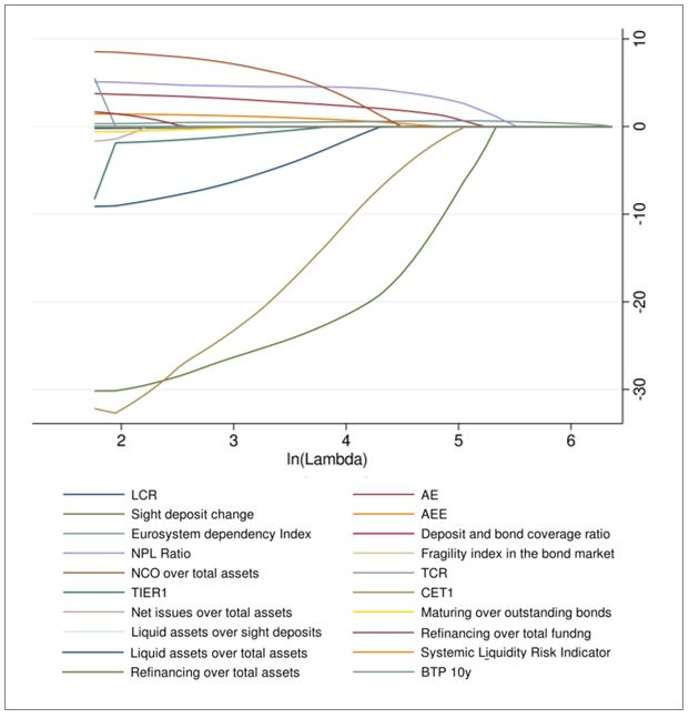
as the largest value for which the mean-squared prediction error is within one standard
error from the minimum loss (Figure A3)17.

The Logistic LASSO has determined the optimal model specification, which in our case
is based on 10 out of the 20 explanatory variables (Figure A4) 18. The first three columns
of Table A5 show the estimates of the Logistic Lasso whereas the last three columns
report the corresponding panel logit model estimates for the LASSO specification
including coefficient standard errors and significance levels, which are not available for
LASSO models. The results appear in line with expectations. Increases in the LCR, sight
deposits change, capital ratios, the ratio between liquid assets and total assets and
improvements in the fragility index on the bond market decrease the probability of a
liquidity crisis in the subsequent 3 months. On the contrary, increases in the AE, the AEE,
the NPL ratio and the net cash outflows over total assets increase this probability. In Table
A5, we also report the estimates for 1- and 2-month forecast horizons as a robustness
check.

Random forest
The random forest method, introduced by Breiman (1996, 2001), is a sophisticated
classification model based on machine learning techniques. To the best of our knowledge,
it has been the most frequently employed machine learning method in the early warning
literature (Tanaka et al., 2016; Holopainen and Sarlin, 2017; Alessi and Detken, 2018). It
is obtained from the aggregation of different classification trees, which represent its
constituent elements.

A decision tree is a very simple and effective method to obtain a classifier and in machine
learning it is used as a predictive model. The aim is to classify accurately the observations
of the dataset based on some input variables. It consists of a root, branches (interior nodes)
and leafs (final nodes). Each node of the tree is associated with a particular decision rule
based on the values of a specific variable and on a threshold . The decision rule assigns
the observations to the right subtree if < and to the left one otherwise. Observations

17
 The lambda that minimizes the mean-squared prediction error is equal to 4.2.
18
 The LASSO model selects the following variables: LCR, Change in sight deposits, AE, AEE, CET1,
 Eurosystem dependency index, NPL Ratio, Fragility index on the bond market, Net cash outflows over
 total assets and the ratio between liquid assets and total assets.

 24

pass through innumerable nodes and reach up to the leaves, which indicate the category
associated with the decision.

Normally a decision tree is built using learning techniques starting from the initial data
set, which can be divided into two subsets: the training set, on which the structure of the
tree is created, and the test set that is used to test the accuracy of the predictive model
created. To estimate a tree, the algorithm chooses simultaneously the variables and
thresholds to split the data, based on a measure of gain from each possible split and some
stopping criteria to limit the complexity of the tree.

When decision trees have a complex structure, they can present overfitting problems on
the training-set and show high variance. For this reason, when building a random forest
it is important to generate a certain heterogeneity between different decision paths by
randomly choosing a subset of observations on which the estimate is carried out (bagging)
and considering only a random subset of attributes at each step (attribute bagging). Both
components are needed in order to sufficiently reduce individual trees correlation and
achieve the desired variance reduction, while maintaining a high degree of prediction
accuracy.

More precisely, the bootstrap creates each time different sub-samples used as training sets
for the construction of a complex decision tree (called weak learner). The data left outside
the training set (out of bag data) are used for tree validation. Randomness becomes part
of the classifiers construction and has the aim of increasing their diversity and thus
diminishing the correlation. This process is repeated randomly N times and the results of
each tree are aggregated together to obtain a single estimate. The aggregated result of the
random forest is nothing but the class returned by the largest number of trees. In this way,
although introducing some distortion, it is possible to reduce drastically the variance of
the estimates thereby having predictions that are more accurate and solving the overfitting
problem.

Analytically, given a set of B identically distributed random variables {Z1,…,ZB} with
 ⁡( , ⁡) = ⁡ ⁡, ( ) = ⁡ ⁡⁡ and ⁡ ⁡( ) = ⁡ 2 ⁡, if we assume that the empirical
 1 ⁡
average is equal to ̅ = ⁡ ∑ then we obtain:

 25

⁡
 2
 ⁡( ̅) = 2 + (1 − ) .
 
Since the random forest model assumes the weak learners are extremely complex trees,
which have high variance but low bias, the main idea is to reduce the variance by
decreasing the correlation between the different trees ( ).

In line with the literature, our random forest aggregates the results of 200 decision trees
and assumes a 3-month forecast horizon. As we have done for the logistic LASSO, to
calculate the threshold value that allows discriminating the crisis events, we applied the
loss function of Sarlin assuming a value of ⁡ ∈⁡(75%, 98%), equivalent to putting a
weight on the false negative outcome (missing a liquidity crisis) between 3 and 49 times
greater than the one of a false alarm.

Extreme Gradient Boosting

The idea of Boosting is similar to the one of the random forest, i.e. improving model
performance by aggregating different weak learners (in our case different decision trees).
This time, however, the selected weak learners have high bias, but low variance. The
boosting method combines them sequentially by working on the residuals of the previous
weak learner. To be more precise, the method starts by adapting a very simple model (in
our case a tree with only two nodes) to the training dataset. Then by looking at the
residuals, it fits another model by giving a higher weight to the observations erroneously
classified and repeats this process until a stopping rule is satisfied. The final output of the
model is obtained by taking a weighted majority vote on the sequence of trees generated.

In contrast with the random forest, the parameters tuning in the Boosting can be extremely
complex. First, it is important to set the number of trees (B) the model is going to use: if
this number is too high, then the model will overfit the data. This parameter must be
selected via cross validation. Second, we need to choose the number of splits (d), which
controls the complexity of the weak learners. By assumption, d must be a small number
since we are interested in weak learners with small variance and high bias. If d = 1 we get
a stump i.e. a tree with only the root. Since by having d splits we will use d attributes at
most, it is useful to consider it as the parameter controlling the level of interaction
between variables that we want to consider. In our case, we set d = 2. Third, the learning
rate, which controls the learning speed of the model, is usually a small positive number,

 26