Proca-stinated cosmology. Part II. Matter, halo, and lensing statistics in the vector Galileon - IOPscience
←
→
Page content transcription
If your browser does not render page correctly, please read the page content below
Journal of Cosmology and
Astroparticle Physics

PAPER • OPEN ACCESS

Proca-stinated cosmology. Part II. Matter, halo, and lensing statistics in
the vector Galileon
To cite this article: Christoph Becker et al JCAP06(2021)014

View the article online for updates and enhancements.

                               This content was downloaded from IP address 46.4.80.155 on 03/08/2021 at 14:04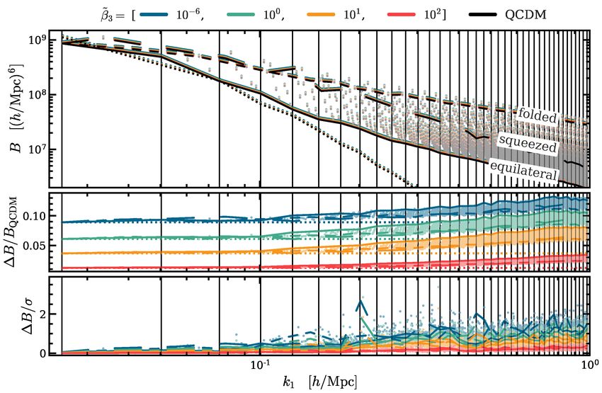
J     ournal of Cosmology and Astroparticle Physics
     An IOP and SISSA journal

Proca-stinated cosmology. Part II.
Matter, halo, and lensing statistics in
the vector Galileon

                                                                                                                      JCAP06(2021)014
Christoph Becker,a,b Alexander Eggemeier,a Christopher T. Daviesa
and Baojiu Lia
a Institute  for Computational Cosmology, Department of Physics, Durham University,
   South Road, Durham DH1 3LE, United Kingdom
 b Institute for Data Science, Durham University,

   South Road, Durham DH1 3LE, United Kingdom
   E-mail: christoph.becker@durham.ac.uk, alexander.eggemeier@durham.ac.uk,
   christopher.t.davies@durham.ac.uk, baojiu.li@durham.ac.uk
Received November 4, 2020
Revised April 14, 2021
Accepted May 20, 2021
Published June 8, 2021

Abstract. The generalised Proca (GP) theory is a modified gravity model in which the ac-
celeration of the cosmic expansion rate can be explained by self interactions of a cosmological
vector field. In this paper we study a particular sub-class of the GP theory, with up to cubic
order Lagrangian, known as the cubic vector Galileon (cvG) model. This model is similar to
the cubic scalar Galileon (csG) in many aspects, including a fifth force and the Vainshtein
screening mechanism, but with the additional flexibility that the strength of the fifth force
depends on an extra parameter — interpolating between zero and the full strength of the
csG model — while the background expansion history is independent of this parameter. It
offers an interesting alternative to ΛCDM in explaining the cosmic acceleration, as well as a
solution to the tension between early- and late-time measurements of the Hubble constant
H0 . To identify the best ways to test this model, in this paper we conduct a comprehensive
study of the phenomenology of this model in the nonlinear regime of large-scale structure
formation, using a suite of N-body simulations run with the modified gravity code ECOSMOG.
By inspecting thirteen statistics of the dark matter field, dark matter haloes and weak lensing
maps, we find that the fifth force in this model can have particularly significant effects on the
large-scale velocity field and lensing potential at late times, which suggest that redshift-space
distortions and weak lensing can place strong constraints on it.

Keywords: cosmological simulations, modified gravity
ArXiv ePrint: 2011.01719

              c 2021 The Author(s). Published by IOP Publishing
             Ltd on behalf of Sissa Medialab. Original content from
this work may be used under the terms of the Creative Commons
Attribution 4.0 licence. Any further distribution of this work must   https://doi.org/10.1088/1475-7516/2021/06/014
maintain attribution to the author(s) and the title of the work,
journal citation and DOI.
Contents

1 Introduction                                                                                  1

2 The generalised Proca (GP) theory                                                             3

3 Cosmological simulations                                                                      5

4 Matter field statistics                                                                       8

                                                                                                     JCAP06(2021)014
  4.1 Matter and velocity power spectra                                                         9
  4.2 Matter bispectrum                                                                        12

5 Halo statistics                                                                              16
  5.1 Halo mass function                                                                       17
  5.2 Two-point correlation functions                                                          18
  5.3 Mean halo pairwise velocity                                                              19
  5.4 Redshift space clustering                                                                20
  5.5 Concentration-mass relation                                                              23

6 Weak lensing statistics                                                                      25
  6.1 Weak lensing convergence and peak statistics                                             25
  6.2 Cosmic voids                                                                             29
      6.2.1 Tunnels                                                                            30
      6.2.2 Watershed                                                                          32

7 Discussion and conclusions                                                                   33

1   Introduction

Understanding the laws of physics that govern cosmic structure formation is indispensable
for probing into the true nature of gravity, because gravity is the dominant one of the four
fundamental forces on cosmological scales. Ever since its establishment, General Relativity
(GR) has been a cornerstone of modern cosmology. Even though the predictions of GR have
been validated against many tests, these tests are usually limited to small scales such as the
solar system [1], leaving the cosmological scales underexplored. The current observational
results of these latter scales, which trace the dynamics of luminous and dark matter such
as stars, galaxies, galaxy clusters, and extended filaments surrounding enormous voids, are
generally in good agreement with the current concordance model of cosmology, ΛCDM,
despite the fact that in recent years a number of tensions between the cosmological parameter
estimates from different observational probes have emerged (e.g., [2–6]]). However, there is
currently no compelling explanation of the smallness of the cosmological constant in this
model, which is why alternative models to explain the cosmic acceleration, such as dynamical
dark energy and modified gravity (MG), have been widely considered. In particular, in most
alternative theories of gravity, the time evolution of large-scale structures can be significantly
influenced, so that the observational data in cosmology may allow accurate tests of such
models on large scales (for a recent review see [7]).

                                              –1–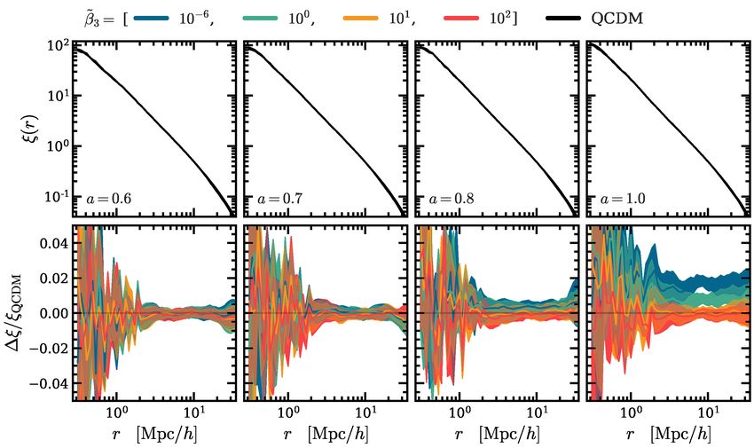
The last decades have seen many attempts to modify GR. According to the Lovelock
theorem, GR is the only theory with second-order local equations of motion for the metric
field, which is derivable from a 4-dimensional action [7], and therefore modifications to GR
often involve new dynamical degrees of freedom in addition to the metric field, non-locality,
higher-dimensional spacetimes and/or higher-order equations. The simplest MG models, for
example, usually involve a single scalar degree of freedom with self-interactions or interactions
with curvature. It has been well-established that such models can be brought under the
umbrella of the Horndeski theory [8–10].
       One of the most well-known subclasses of the Horndeski theory is the Galileon model [11–
13], a 4-dimensional effective theory which involves a scalar field with universal coupling to

                                                                                                    JCAP06(2021)014
matter and derivative self-interactions. The theory implements Vainshtein screening [14] — a
nonlinear mechanism also encountered in theories such as Fierz-Pauli massive gravity [15] and
the Dvali-Gabadadze-Porrati (DGP) model [16] — to decouple the scalar field from matter
near massive objects and therefore can be compatible with Solar system tests of gravity. The
model modifies the background expansion history such that it reaches a de Sitter solution
in the future without requiring a cosmological constant. Its simplicity makes it possible to
study its phenomenology with the help of cosmological N -body simulations [17, 18]. We refer
to this model as the scalar Galileon below.
       In contrast to the scalar Galileon, the generalised Proca theory (GP) [19–21], involves a
massive vector field, Aµ , with a broken U(1) gauge symmetry and second-order equation of
motion (EOM). The theory features Galileon-type derivative self-interactions and couplings
to matter. At the background level, the temporal component of the vector field, A0 , gives
rise to a self-accelerating de Sitter attractor, corresponding to a dark energy equation of
state wDE = −1 [22]. From the gravitational wave event GW170817 [23] with accompanying
gamma-ray burst GRB170817A [24] and other optical counterparts, the speed of propagation
of the gravitational waves cT has been tightly constrained to be identical to the speed of
light, c. This places strong constraints on the allowed operators within the higher order
GP Lagrangian. However, even with this restriction, the GP theory is still cosmologicaly
interesting, with a theoretically consistent parameter subspace that is free of ghost and
Laplacian instabilities [22], and in which cT = c.
       By introducing non-linear functions into the field Lagrangian of the GP theory to de-
scribe its derivative self interactions and couplings with matter, it can be very versatile and
flexible. However, in cosmological applications one often specialises to simple choices of these
non-linear functions, such as power-law functions, and a number of studies have been con-
ducted along this direction, leading to a good understanding of the cosmological behaviours
of the model at background and linear levels. For example, in refs. [25, 26], Markov Chain
Monte Carlo likelihood analyses were performed for the particular GP theories proposed in
refs. [22, 27], by exploiting the observational data from type Ia supernovae (SNIa), the cosmic
microwave background (CMB), baryonic acoustic oscillations (BAO), the Hubble expansion
rate H(z), and redshift-space distortions (RSD). The cross correlation between galaxy field
and the integrated Sachs Wolfe (ISW) effect, which has been a powerful probe to constrain
the scalar Galileon models, has also been used to constrain parameters of the GP theory [28].
       In this work, we conduct a broad phenomenological study of a set of five cosmologies
based on the toy GP model studied in [29]. Using the N -body code developed in [29] and
augmenting it with an independent set of ray-tracing modules taken from Ray-Ramses [30], we
can supplement previous results with the measurements of non-linear scales and unexplored
statistics of the matter field, haloes, weak lensing, and voids. There are several motivations

                                             –2–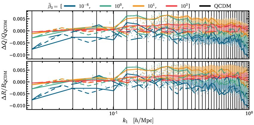
for doing so. One is that we know perturbation theory is not good at quantifying the effects of
screening, which is an inherently non-linear phenomenon. N -body simulations are the only
known tool to accurately study the evolution of the Universe on small, highly non-linear,
scales, and can be used to validate or calibrate the predictions of other approaches. Being
able to probe small scales (k & 1 h/Mpc) will enable us to test a given model against more
observational data more accurately, e.g., access scales or regimes that are inaccessible to
perturbation theory. For this reason, we will analyse a total of 13 matter, halo, weak lensing
and void statistics, in the effort to identify the ones which are most sensitive to the effect of
the fifth force in the GP theory.
      This paper is arranged as follows. In section 2 we introduce the GP theory and the
particular instances of it that we will focus on in this work. In section 3 we describe the set

                                                                                                    JCAP06(2021)014
up of the N -body and ray-tracing simulations on which all following results are based. This
is followed by presentations of the main results of the dark matter field (section 4), haloes
(section 5), and weak lensing (section 6). Finally, we summarise and discuss in section 7.
      Throughout this paper, we will use the (−, +, +, +) signature of the metric and abbrevi-
ations ∂A = ∂µ Aµ , (∂A)2 = ∂µ Aµ ∂ν Aν . We set c = 1 except in expressions where c appears
explicitly. Greek indices run over 0, 1, 2, 3 while Roman indices run over 1, 2, 3.

2   The generalised Proca (GP) theory

In this work, we study the generalised Proca theory of gravity, the most general vector-tensor
theories with second-order equations of motion, which contains Lagrangian operators up to
cubic order of the Proca field. The action of this model is given by
                                         "                             #
                                     √                    M2
                            Z
                       S=       d x −g Lm + LF + L2 + L3 + Pl R ,
                                 4
                                                                                            (2.1)
                                                           2

where g denotes the determinant of the metric tensor gµν , Lm is the matter Lagrangian
density, LF,2,3 are the Lagrangian operators introduced by the Proca field, Aµ , and the last
                                                                            −2
operator is the standard Einstein-Hilbert term with the Planck mass, MPl       = 8πG, G is
Newton’s constant, and R is the Ricci scalar. The Proca field can be decomposed as

                                 Aµ = (A0 , Ai ) = (ϕ, Bi + ∇i χ),                          (2.2)

where ϕ is the temporal component of the vector field, Bi is its transverse mode which is
divergence free, ∇i Bi = 0, and χ is the longitudinal scalar (which can also be referred to as
the scalaron field)
      The matter Lagrangian density is related to the energy-momentum tensor of a perfect
fluid as,                                          √
                                             2 δ( −gLm )
                                   (m)
                                 Tµν   = −√                  ,                           (2.3)
                                             −g     δg µν
which, assuming that matter is minimally coupled to gravity, satisfies the standard conser-
vation equation
                                     ∇µ Tµν
                                          (m)
                                              = 0,                                    (2.4)
where ∇µ denotes the covariant derivative compatible with gµν .
    Introducing the first derivative of the vector field, Bµν = ∇µ Aν , we can build the anti-
symmetric Faraday tensor as Fµν ≡ Bµν − Bνµ . The kinetic term of the Proca Lagrangian,

                                              –3–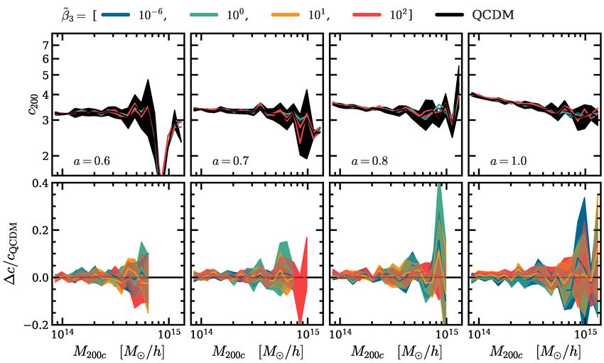
LF , can be described as,
                                               1
                                      LF = − Fµν F µν ,                                     (2.5)
                                               4
and the self-interaction terms of the vector field are given by,
                 L2 = G2 (X) = b2 X p2 ,     L3 = G3 (X)∇µ Aµ = b3 X p3 ∇µ Aµ ,             (2.6)
where X ≡ 12 gµν Aµ Aν , b2 ≡ m2 is the mass-squared of the vector field that characterises
the onset of the acceleration epoch, and b3 , p2 , p3 are parameters of mass dimension zero in
natural units. The choice is generic enough, leaving a viable parameter space in which the
theory is free of ghost and Laplacian instabilities [22]. Importantly, due to the derivative
self-interaction of the vector field in L3 , the gravitational effect of the field can be screened

                                                                                                     JCAP06(2021)014
in dense regions as required by solar system tests. The screening mechanism in this model
is analogous to the Vainshtein mechanism [31]. In this work we set p2 = p3 = 1 as a working
example to study the qualitative behaviour of the Proca field and refer to it from now on as
cubic vector Galileon (cvG). With this choice, the GP theory behaves as the standard cubic
scalar Galileon model (csG) in certain limits [29].
      When deriving the equation of motions (EOM), we consider the perturbed Friedmann-
Robertson-Walker metric in the Newtonian gauge
                        gµν = −(1 + 2Ψ)dt2 + a2 (t)(1 − 2Φ)δij dxi dxj ,                    (2.7)
where a(t) is the time-dependent scale factor which is normalised to a(t0 ) = 1 at the present
day, and δij = diag(+1, +1, +1) represents the spatial sector of the background metric that
is taken here to be flat, k = 0.
      As shown in [29], we expect the ‘back-reaction’ of Bi on the evolution of χ and Φ to be
very small, justifying the neglect of the B i field in the simulations. To perform cosmological
simulations for this model, we rewrite all required equations in ECOSMOG’s code units, which
we indicate as tilded quantities (details in [29]). The equations are then rescaled through
                                                3βsDGP 0
                                         χ̃ =         χ̃ ,                                  (2.8)
                                                  2β
to make an educated choice of the cvG model parameter possible, by comparing it with the
well studied sDGP model (for more details see [29]). To lighten our notation, we will drop
the prime in χ̃0 .
      The modified Friedman equation, which depends on the EoM of ϕ at the background
level, given by
                                            H 2 β̃2
                                      ϕ = 20        ,                                 (2.9)
                                           3c H β̃3
is
                            H(a) 2 1
                                                   q
                                              −3
                       2
                     E ≡            =    Ωm a + Ωm a + 4ΩP ,
                                                        2 −6                        (2.10)
                             H0       2
where H(a) is the Hubble expansion rate at a, H0 = H(a = 1), Ωm is the matter density
parameter, and ΩP the Proca field density parameters today,
                                           ΩP ≡ 1 − Ωm .                                   (2.11)
     We have considered only non-relativistic matter; the inclusion of radiation and massive
neutrinos is straightforward. Therefore, the background expansion history in this model is
completely determined by H0 and Ωm .

                                                –4–
The modified Poisson equation, rescaled by eq. (2.8), under the quasi-static approxima-
tion and in the weak-field limit takes the following form in code units,
                                          3                3βsDGP ˜2 0
                                  ∂˜2 Φ̃ = Ωm a (ρ̃ − 1) +       α∂ χ̃ ,                            (2.12)
                                          2                  2β
where ρ̃ is the matter density in code unit, βsDGP is the coupling strength between matter and
the brane-bending mode in the sDGP model, and α and β are two time-dependent functions
given by
                               1
                                               q
                                      1/3 −1/3                          −3
                     α(a) = √       β̃3 ΩP        Ωm a + 4ΩP − Ωm a
                                                    2 −6                     ,          (2.13)
                             232

                                                                                                              JCAP06(2021)014
and                                  !1/3 "
                          1                               3Ω2m a−6
                                                                       #
                                β̃3              −3
                  β(a) =                    5Ωm a + p 2 −6               + β̃3 ,        (2.14)
                          2 2ΩP                         Ωm a + 4ΩP
which are both fully fixed by specifying Ωm and the coupling constant b3 redefined as
β̃3 ≡ b3 (8πGH02 )/c6 [29].
      Finally, the EOM for the longitudinal mode of the Proca field, χ, in the weak-field limit
and rescaled by eq. (2.8),
                            1      ˜2 χ̃0 − ∂˜i ∂˜j χ̃0 ∂˜i ∂˜j χ̃0 = 1 Ωm a (ρ̃ − 1) ,
                                       2
               ∂˜2 χ̃0 +

                                   ∂                                                                (2.15)
                           3γa4                                       βsDGP
where the source term on the right-hand side is identical to that in the sDGP equation [32],
and we have defined a new time-dependent function
                                                        2β 2
                                           γ(a) ≡                ,                                  (2.16)
                                                    9βsDGP Rc2
with the following dimensionless and time-dependent function
                                 1 2/3
                                                        q
                      Rc2 (a)   = β̃3 (2ΩP )−2/3 Ωm a−3 + Ω2m a−6 + 4ΩP .                           (2.17)
                                 2
Thus, given a matter density field, we can solve for the scalaron field χ from eq. (2.15) and
plug it into the modified Poisson equation eq. (2.12) to solve for Φ̃. Once Φ̃ is at hand, we can
use finite-difference to calculate the modified gravitational force, which determines how the
particles move subsequently. Note that, in this model, Φ̃ not only determines the geodesics
of massive particles, but also those of massless particles such as photons — in other words,
the lensing potential is also modified.
      As β̃3 is the only ‘free’ parameter that enters in all three key equations, it is practical
to use it as the model parameter.

3       Cosmological simulations
In this section we present the set of dark-matter-only simulations for five different cosmologies
which we use to investigate the phenomenology of the cvG model. Their basic configuration
is shown in table 1. Four of these take different values of the model parameter of the cvG
model, β̃3 = [10−6 , 100 , 101 , 102 ], and one is their QCDM counterpart,1 in the simulation.
    1
    This is a variant that only considers the modified background expansion history, but uses standard New-
tonian gravity to evolve particles.

                                                    –5–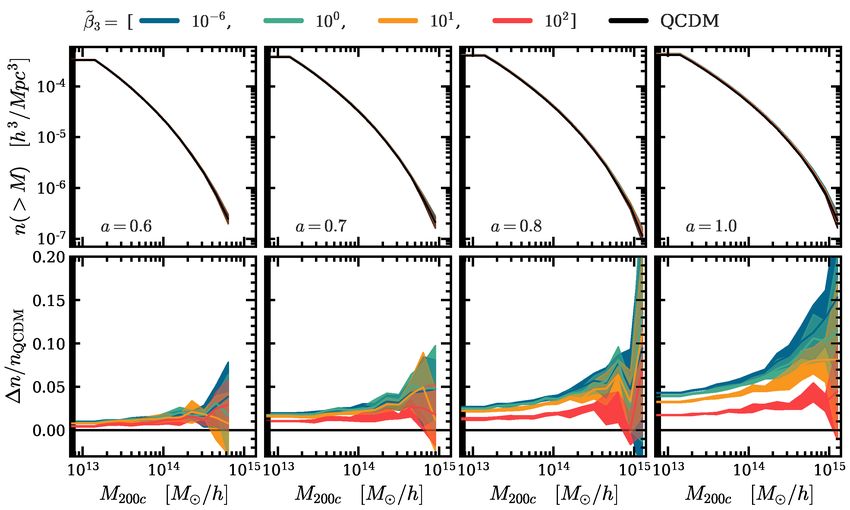
It is equivalent to the limit β̃3 → ∞ [29]. To study the cvG effects on the weak lensing
(WL) signal, we extended the N -body code developed in the previous work [29] by adding
an independent set of ray-tracing modules taken from Ray-Ramses [30]. This allows us to
calculate the WL signal ‘on-the-fly’ as proposed by [33, 34], while taking full advantage of
the time and spatial resolution available in the N -body simulation.
      We construct a light-cone for each cosmology by tiling a set of five simulation boxes,
all having an edge-length of Lbox = 500h−1 Mpc, as shown in figure 1. The simulations
treats dark matter as collisionless particles described by a phase-space distribution function
f (x, p, t) that satisfies the Vlasov equation

                         df   ∂f    p                      ∂f

                                                                                                     JCAP06(2021)014
                            =    +      2
                                          · ∇f − m0 (∇Ψ) ·    = 0,                          (3.1)
                         dt   ∂t   m0 a                    ∂p

where p = a2 m0 ∂x/∂t, m0 is the particle mass, and Ψ is the modified Newtonian potential
given by eq. (2.12). Note that, as we do not include matter species such as photons and
massive neutrinos the two Bardeen potentials are equivalent, Ψ = Φ. The exclusion of
photons should not have a noticeable impact on our simulations, which are only run at low
redshifts. The impact of neglecting massive neutrinos depends on the neutrino mass, and
for the currently allowed mass range, we do not expect qualitative changes. We plan to run
simulations by including massive neutrinos in the future. Hence to solve Ψ, and prior to it
the longitudinal Proca mode, via eq. (2.15), they are discretised and evaluated on meshes
using the nonlinear Gauss-Seidel relaxation method [32]. The domain grid — which is the
coarsest uniform grid that covers the entire simulation box — consists of Ngrid = 5123 cells,
which is equal to the number of tracer particles, Np . ECOSMOG is based on the adaptive-
mesh-refinement (AMR) code RAMSES [35], which allows mesh cells in the domain grid to be
hierarchically refined — split into 8 child cells — when some refinement criterion is satisfied.
In our simulations, a cell is refined whenever the effective number of particles inside it exceeds
8. This gives a higher force resolution in dense non-linear regions, where the Vainshtein
screening becomes important. The Gauss-Seidel algorithm is run until the difference of the
two sides of the PDE, dh , is smaller than a predefined threshold . We verified that for a
value of  = 10−9 > |dh |, the solution of the PDE no longer changes significantly when  is
further reduced.
      We use the same set of five different initial conditions (ICs), for each of the five sim-
ulations that make up a light-cone for a given cosmology are different, for the different
cosmologies. The ICs were generated using 2LPTic [36], with cosmological parameters taken
from the Planck Collaboration [37],

          h = 0.6774,    ΩΛ = 0.6911,    Ωm = 0.389,     ΩB = 0.0223,     σ8 = 0.8159.      (3.2)

The linear matter power spectrum used to generate the ICs is obtained with CAMB [38]. The
simulation starts at a relatively low initial redshift zini = 49, or aini = 0.02, justifying the
use of second-order Lagrangian perturbation theory codes such as 2LPTic. One possible
concern may be that, at this scale factor, differences of matter clustering are already present.
However, judging from our experience [29], at this time the difference between the growth
factors of the cvG model with ΛCDM is well below sub-percent level, so that modified effects
on the initial matter clustering can be neglected. Additionally, it has been shown that ICs
generated with 2LPTic at zini = 49 can produce accurate matter field statistics for our
simulation size and resolution at z = 0 [36].

                                              –6–
Lbox          Nr. of particles           kNy          force resolution       convergence
                 500   h−1 Mpc            5123           3.21 h/Mpc           30.52 h/kpc        || < 10−12 /10−9

Table 1. Summary of technical details that are identical for all simulations performed for this
work. Here kNy denotes the Nyquist frequency.  is the residual for the Gauss-Seidel relaxation
used in the code [39], and the two values of the convergence criterion are for the coarsest level and
refinements respectively.

                                                                       z
                       0      0.09      0.17     0.27     0.37        0.47    0.58    0.70       0.83   0.97      1.12
                 500

                                                                                                                             JCAP06(2021)014
ycoord [Mpc/h]

                 250

                   0
                       0                500               1000                1500               2000             2500
                                                             zcoord [Mpc/h]
Figure 1. Light-cone layout. The light cone (solid blue line) is made up of five simulation boxes (red
squares). All simulated boxes have a side length of 500h−1 Mpc and the light cone has an opening
angle of 10 × 10 deg2 . The comoving distance to the observer and redshift are respectively labelled in
the lower and upper axes. The vertical dotted lines, which are at distances equal to 1/4 and 3/4 times
the box size from the nearer side of each box, correspond to the redshifts at which particle snapshots
are outputted.

       The light-cone, outlined by solid blue lines in figure 1, is constructed by positioning the
five simulation boxes, outlined by solid red lines in figure 1, relative w.r.t. the observer. The
geometrical set-up was constructed to place the sources at zs = 1, which is the starting point
when the growth rate of matter density perturbations becomes higher than in ΛCDM [29].
The field-of-view (FOV) is set to 10 × 10 deg2 (so that the wide end of the light-cone is
still narrow enough to fit in the simulation box), within which 2048 × 2048 rays are followed
by Ray-Ramses to compute quantities of interest. Ray-Ramses is an on-the-fly ray-tracing
code. The rays are initialised when a given simulated box reaches a defined redshift (for the
closest and furthest box to the observer the initialisation redshift is respectively zi = 0.17
and zi = 1.0), and end after they have traveled the covered length of the box, meaning
500h−1 Mpc. As here we are interested in the lensing convergence, κ, the quantity that is
computed along the rays is the two-dimensional Laplacian of the lensing potential,

                                         ˜ 2 Φ̃lens,2D = ∇
                                         ∇               ˜ 1∇
                                                            ˜ 1 Φ̃lens,2D + ∇
                                                                            ˜ 2∇
                                                                               ˜ 2 Φ̃lens,2D ,                       (3.3)

where 1, 2 denote the two directions on the sky perpendicular to the line of sight (LOS).
The values of these two-dimensional derivatives of Φlens,2D can be obtained from its values at
the centre of the AMR cells via finite differencing and some geometrical considerations (see
refs. [30, 34]). Integrating this quantity as

                                           1          χ (χs − χ) ˜ 2
                                                 Z χs
                                        κ= 2                                    ~
                                                                ∇ Φ̃lens,2D (χ, β(χ))dχ,                             (3.4)
                                          c       0        χs

                                                                 –7–
where c is the speed of light, χ is the comoving distance, χs the comoving distance to the
                      ~
lensing source, and β(χ)   indicates that the integral is performed along the perturbed path
of the photon (χ is not to be confused with the longitudinal mode of the Proca field). The
integral is split into the contribution from each AMR cell that is crossed by a ray, which
ensures that the ray integration takes full advantage of the (time and spatial) resolutions
attained by the N -body run. For the WL signal we wish to study in this paper, we employ
the Born approximation, in which the lensing signal is accumulated along unperturbed ray
trajectories. We will make further notes on the calculations in section 6.1.

4       Matter field statistics

                                                                                                                                           JCAP06(2021)014
In this section we present the results of various dark matter statistics of the different cvG
models and compare them with the predictions by QCDM, to study the impact of the Proca
field on these key observables. We start with an analysis of the power spectra in Section 4.1.
In section 4.2, we consider the leading non-Gaussian statistic in large-scale structure cluster-
ing, the bispectrum, which is thus sensitive to deviations from linear evolved perturbations
from single field inflation.
      To support the analysis and interpretation of the results, we will compare the results
of the N -body simulations to Eulerian standard perturbation theory (SPT), and limit the
comparison only to the tree-level statistics. In SPT, the energy and momentum conservation
equations can be solved order by order to obtain higher-order corrections to the quantities
of interest. The expansion in powers of the linear density field is a simple time dependent
scaling of the initial density field (in the Einstein de Sitter approximation),
                                                                  ∞
                                                    δ(k, τ ) =          Dn (τ )δ (i) (k),                                          (4.1)
                                                                  X

                                                                  i=1

for which the n-th order solution is
                      Z
    δ   (n)
              (k) ∼       d3 k1 . . . d3 kn δ (D) (k − k1...n )Fn (k1 , . . . , kn )δ (1) (k1 , τini ) . . . δ (1) (kn , τini ),   (4.2)

with the conformal time τ = dt/a, k1...n ≡ k1 + . . . + kn , the density contrast δ = ρ/ρ̄, δ (D)
                                              R

the 3D Dirac delta function, and Fn the SPT fundamental mode coupling kernel [40, 41].
      When comparing a cvG model to the QCDM counterpart, we do so through their relative
difference which we write in short hand as
                                                       ∆A            AX − AQCDM
                                                                 ≡              ,                                                  (4.3)
                                                    AQCDM              AQCDM
with A a placeholder of the summary statistics, and X will be one of the four cvG models.
We calculate ∆A/AQCDM for each of the five pairs of cvG and QCDM simulations that
share the same initial conditions to find its average and 1σ uncertainty. Taking this ratio
removes contributions from cosmic variance, and so its uncertainty is not a direct indicator
of how sensitive the various summary statistics are to differences between the cvG models.
To provide an estimate of this sensitivity given a survey volume as large as our simulation
box, we calculate the signal-to-noise ratio (SNR) of the difference between cvG models and
their QCDM counterpart for some summary statistics using the expression
                                                            ∆A  AX − AQCDM
                                                  SNR ≡        =q           ,                                                      (4.4)
                                                             σ    2 + σ2
                                                                 σX    QCDM

                                                                     –8–
where ∆A is the average and σ is the standard deviation of the five simulations per cosmo-
logical model. We note that the SNR values obtained in this way could be subject to sample
variance, owing to the small number of realisations. This is not a problem for the qualitative
study presented in this paper, but more simulation volume is needed before we can place
reliable quantitative constraints on this model. This will be left for future work.
4.1 Matter and velocity power spectra
To gain insights into the differences of matter clustering and peculiar velocities on linear and
nonlinear scales among the various models in this work, we begin our study of dark matter
phenomenology by considering the auto power spectra of the matter over-density, δ, given by
JCAP06(2021)014
hδ(k1 , t)δ(k2 , t)i = (2π)3 δ (D) (k1 + k2 )Pδδ (k1 , t). (4.5)
Cosmic structure formation is driven by the spatially fluctuating part of the gravitational
potential, Φ(x, t), in eq. (2.7), induced by the density fluctuation δ. In cvG cosmologies we
expect an additional boost to the standard gravitational potential with respect to its QCDM
counterpart, induced by χ described by eq. (2.12), in regions where the fifth force is not
screened by the Vainshtein mechanism. Thus, clustering will be enhanced in the cvG models
on some scales, which can be captured by Pδδ .
The top row of figure 2 compares the linear matter power spectra (black dotted lines)
with the simulation results of each cosmology (coloured lines with shaded regions), at a = 0.6
(outer left), a = 0.7 (inner left), a = 0.8 (inner right), and a = 1.0 (outer right). The linear
(11)
power spectrum, Pδδ (k; z), is obtained by multiplying the initial matter power spectrum at
zini = 49, Pδδ (k; zini ), with [D(z)/D(zini )]2 . The nonlinear matter power spectra are measured
from particle snapshots using the POWMES2 code [42]. The mean Pδδ of the five realisations
per cosmology is shown as a coloured line while the standard deviation is indicated as shaded
region. The standard deviation is largest at large scales (k . 0.1 h/Mpc) due to cosmic
variance and the limited simulation size. The vertical shaded region near the right edge of
each panel indicates the regime of k beyond the Nyquist frequency.3
The centre row of figure 2 shows the relative differences, eq. (4.3), of the matter power
spectra. The relative difference has been smoothed to remove noise at scales k > 0.2 h/Mpc,
using a Savitzky-Golay filter of second order with a kernel width of 13 data-points [43]. The
power spectrum results agree with the results found in ref. [29] and extend them by including
larger scales and measurement uncertainties.
The bottom panel of figure 2 shows the SNR of the difference between cvG cosmologies
and their QCDM counterpart. From it we can see that the SNR is larger at large k as σ is
smaller, reflecting the fact that more Fourier modes can be sampled in that k regime. This
implies that the effects of the cvG model are stronger on smaller, more non-linear scales,
and for smaller β̃3 values. However, note that the matter power spectrum is not directly
observable, and later in this paper we will look at the behaviours of quantities more directly
related to observables, such as the lensing power spectrum and halo correlation function.
The real-space position of tracers of the matter distribution are not directly measurable,
preventing us from comparing Pδδ to observations, which rely on the redshift measurement to
infer distances. The reason is that peculiar velocities (i.e., additional velocities to the Hubble
2
The code is in the public domain, https://www.vlasix.org/index.php?n=Main.Powmes.
3
Note that the Nyquist frequency, kNy , marks the absolute maximum up to which we can the power
spectrum can be trusted.
–9–β̃ 3 = [ 10 −6 , 10 0 , 10 1 , 10 2 ] QCDM
104
Pδδ [Mpc 3 /h 3 ]
103
102
101 a = 0.6 a = 0.7 a = 0.8 a = 1.0
0.08
JCAP06(2021)014
∆Pδδ /Pδδ, QCDM
0.06
0.04
0.02
0.00
10
∆Pδδ /σ
0
10-2 10-1 100 10-2 10-1 100 10-2 10-1 100 10-2 10-1 100
k [h/Mpc] k [h/Mpc] k [h/Mpc] k [h/Mpc]
Figure 2. The matter power spectrum in the cvG model. Each column shows the results for a
different scale factor: outer left: a = 0.6, inner left: a = 0.7, inner right: a = 0.8, outer right:
a = 1.0. Top: the matter power spectrum of linear perturbation theory (dotted) and the cvG model
for four values of β̃3 = (10−6 , 1, 10, 100), indicated by a blue, green, orange and red line respectively.
Centre: relative differences between the matter power spectra of the cvG and QCDM models. A
Savitzky-Golay filter has been used to smooth ∆Pδδ (k)/Pδδ,QCDM (k) for k > 0.2 h/Mpc. Each panel
compares linear perturbation theory (black dotted), to results obtained from full simulation (coloured
solid). The vertical grey shaded region in each panel indicates where k > kNy where kNy is the
Nyquist frequency. Bottom: the signal-to-noise ratio of the difference between the cvG models and
their QCDM counterpart.
flow) of the tracers distort the redshift signal along the line of sight. Thus, Pδδ is different
from its counterpart in redshift space, Pδδ
s , which becomes anisotropic despite the statistical
istropy of the Universe; on large scales the two are related by the linear Kaiser formula
2
s
Pδδ (k, µ) = 1 + f µ2 Pδδ (k), (4.6)
where µ is the angle between the wavevector and the LOS, and f is the linear growth rate
defined as f = d(lnδ)/d(lna).
The Kaiser formula can be improved down to quasi linear scales with additional infor-
mation about the auto power spectrum of the velocity divergence,4 θ = ∇ · v, denoted as
4
Strictly speaking, one should consider the complete velocity field, which would also involve its vorticity
∇i × vi . However, just as the transverse mode of the Proca field, ∇i × Bi , it has a much smaller magnitude
than its divergence and is thus neglected in SPT.
– 10 –JCAP06(2021)014
Figure 3. The velocity divergence power spectrum in the cvG model. Each column shows the results
for a different scale factor: outer left: a = 0.6, inner left: a = 0.7, inner right: a = 0.8, outer right:
a = 1.0. Top: the velocity divergence power spectrum of linear perturbation theory (dotted) and the
cvG model for four values of β̃3 = (10−6 , 1, 10, 100), indicated by a blue, green, orange and red line
respectively. Bottom: relative differences between the velocity divergence power spectra of the cvG
and QCDM models.
Pθθ , as well as their cross spectrum Pδθ , since the velocity field is more sensitive to tidal
gravitational fields compared to the density field on large scales [44–46].
The first row of figure 3 compares the linear velocity divergence power spectrum (black
dotted lines) and measured nonlinear (coloured) simulations, at a = 0.6 (outer left), a = 0.7
(inner left), a = 0.8 (inner right), and a = 1.0 (outer right). The linear power spectrum
(11) (11)
Pθθ (k; z) can be related to Pδδ (k; z) through the zeroth-moment of eq. (3.1), yielding the
continuity equation,
1
δ̇ + ∇ · [v (1 + δ)] = 0. (4.7)
a
On linear scales we can assume that the quadratic terms in eq. (4.7) vanish leaving use with
θ = −aδ̇ = −aHf δ. (4.8)
Thus, the linear power spectrum of the velocity divergence is given by
(11) (11)
Pθθ (k; z) = (aHf )2 Pδδ (k; z). (4.9)
This relation is expected to fail on non- and quasi-linear scales, as velocities grow more slowly
(11)
than the linear perturbation theory predicts. Therefore, any differences in Pθθ between the
different cvG models will appear on these scales.
– 11 –In order to measure the non-linear Pθθ from the numerical simulations, we first use a
Delaunay tessellation field estimator (DTFE,5 [47]) to obtain the volume weighted velocity
divergence field on a regular grid. This procedure constructs the Delaunay tessellation from
the dark matter particle locations and interpolates the field values onto a regular grid, defined
by the user, by randomly sampling the field values at a given number of sample points within
the Delaunay cells and then taking the average of those values. For our 500h−1 Mpc simulation
boxes, we generate a grid with 5123 cells. From that we then measure Pθθ using the public
available code nbodykit6 [48].
We can see from the top row of figure 3 that the results of the simulations for all models
have approached the linear theory prediction on scales k . 0.1 h/Mpc for all times. On
these scales, the time evolution of the power spectrum of all models is scale independent and,
JCAP06(2021)014
(11)
the relative difference encapsulates the modifications to the time evolution of Pθθ via H
and f in eq. (4.9). On smaller scales, the formation of non-linear structures tends to slow
down the coherent (curl-free) bulk flows that exist on larger scales. This leads to an overall
suppression of the divergence of the velocity field compared to the field theory results for
scales k & 0.1 h/Mpc.
A careful look into the relative difference ∆Pθθ (k)/Pθθ,QCDM (k) in the bottom row of
figure 3 also reveals a number of other interesting features on all scales. Firstly, we see
that the wavenumber at which linear theory and simulation results for ∆Pθθ (k)/Pθθ,QCDM (k)
agree, k∗ , depends both on β̃3 and the scale factor. The value of k∗ is pushed to ever larger
scales as a → 1 and β̃3 → 0. A similar observation has been made by [32] for the DGP
model. This is important for the growth rate measurement from redshift distortions, because
it gives useful information about on which scales we can extract the growth rate based on
the predictions of linear perturbation theory. Secondly, on small scales, k & 1 h/Mpc, we
can see how deviations from QCDM are suppressed by the screening mechanism, reflecting
the fact that inside dark matter haloes the screening is very efficient. As also shown by
∆Pδδ (k)/Pδδ,QCDM (k), the screening mechanism becomes more effective as β̃3 → 0. Thirdly,
for a → 1 and β̃3 → 0 we see a growing peak that for the case of β̃3 = 10−6 protrudes above
the linear theory prediction at k ∼ 0.7 h/Mpc. A similar feature was also observed by [32]
for the DGP model.
The difference of Pθθ between the cosmological models compared to its magnitude is
very small at early times, e.g., at percent level for all models when a . 0.6, but increases
rapidly over time, reaching 35% for β̃3 = 10−6 at a = 1.0. This is unlike the behaviour of
∆Pδδ (k)/Pδδ,QCDM (k) which increases much more slowly and only reaches ∼ 5% for β̃3 =
10−6 at a = 1.0. This difference is because the velocity field, being the first integration of the
forces, responds more quickly to a rapid growth of the fifth-force magnitude than does the
matter field, which is the second integration of the forces. It shows the rapid increase of the
linear growth rate of the cvG model at late times (a & 0.8), and suggests that redshift-space
distortions (RSD) in this time window can be a strong discriminator of this model.
4.2 Matter bispectrum
As we have mentioned, even if cosmological fields are initially Gaussian, they inevitably de-
velop non-Gaussian features as the dynamics of gravitational instability is nonlinear. Conse-
quently, the structures found in the density field can no longer be fully described by two-point
5
The code is in the public domain, http://www.astro.rug.nl/~voronoi/DTFE/dtfe.html.
6
The code is in the public domain, https://nbodykit.readthedocs.io.
– 12 –statistics alone, and higher-order correlation functions are needed in order to unlock addi-
tional information, in particular regarding the nature of gravitational interactions. To obtain
first impressions of this information we use the Fourier space counterpart of the three-point
correlation function, the bispectrum, which is receiving increased attention in the recent lit-
erature, not only for making more accurate predictions (see, e.g., [49–52]), but also as a probe
of effects beyond ΛCDM (e.g. [53–59]).
We restrict ourselves to the study of the matter field in real space at z = 0, for which
the bispectrum is given by
hδ(k1 )δ(k2 )δ(k3 )i = (2π)3 δ (D) (k1 + k2 + k3 )B(k1 , k2 , k3 ), (4.10)
JCAP06(2021)014
with the three wave vectors forming a closed triangle. As the study of the effects on bis-
pectrum due to modifications to GR are still in its infancy, we shall be as comprehensive as
possible by considering all possible triangle configurations between the two extreme scales
kmin and kmax , given a specific bin width ∆k1 = |∆k1 | for each side. A detection of strong
configuration dependence can be regarded as a compelling motivation to further investigate
higher-order statistics. It would allow us to disentangle the modified gravity signal from
other potential cosmological effects, which might be degenerate in two-point statistics and
other alternative measures.
The top panel of figure 4 compares the bispectrum of equilateral triangles at the tree-
level (dotted line), to the measurements (solid line). It furthermore contains the measured
bispectrum of squeezed triangles (long dashed), folded triangles (short dashed), and all other
triangle configurations (scattered dots). Vertical lines are spaced ∆k = |∆k| apart. As
we assume a primordial Gaussian random field, we can apply the Wick theorem to write
the bispectrum as products of power spectra summed over all possible pairings. Thus, the
lowest-order bispectrum that is able to capture non-Gaussian features at late times has to
expand one of the fields in the correlator of three Fourier modes to second order, yielding
B (211) (k1 , k2 , k3 ) = hδ (2) (k1 )δ (1) (k2 )δ (1) (k3 )i0 + cyc. = 2F2 (k1 , k2 )P (11) (k1 )P (11) (k2 ) + cyc.,
(4.11)
where δ is given in eq. (4.2), the primed ensemble average indicates that we have dropped
(n)
the factor of (2π)3 as well as the momentum conserving Delta function, and “cyc.” stands for
the two remaining permutations over k1 , k2 and k3 . Note here, that we have assumed that
SPT gives an appropriate description of perturbations in the cvG model and does not fail
to include further mode couplings that might be introduced through the additional Proca
vector field. We will see below that this is indeed an excellent approximation. The resulting
bispectrum scales as square of the linear power spectrum, P (11) , and exhibits a strong con-
figuration dependence as it is directly proportional to the second-order perturbation theory
kernel, F2 , which is given by,
17 1 k1 · k2 k2 k1 2 (k1 · k2 )2 1
" #
F2 = + + + − . (4.12)
21 2 k1 k2 k1 k2 7 k12 k22 3
To measure the bispectrum from the simulations, we first use fourth-order density in-
terpolation on two interlaced cubic grids [60] of N = 256 cells per side. Next, we measure
B(k1 , k2 , k3 ) using an implementation of the bispectrum estimator presented in ref. [61].
Starting from kmin = 2kf = 0.025 h/Mpc, where kf denotes the fundamental mode, we loop
through all configurations satisfying k1 > k2 > k3 and k1 ≤ k2 + k3 (the triangle closure
– 13 –JCAP06(2021)014
Figure 4. Top: real-space bispectrum measurements for cvG cosmologies (coloured points) and their
QCDM counterpart (black points). Each data point corresponds to one of 5910 triangle configurations
(see the text for more details). The vertical lines are spaced by the bin width ∆k ≈ 0.025 h/Mpc and
indicate the value of |k1 |, i.e., the largest triangle side. The bispectrum for equilateral configurations
are shown at the tree-level (dotted), B211 , and simulation measurement (solid). The measured bispec-
tra for the squeezed and folded configurations are shown as long and short dashed lines respectively.
Middle: the relative difference between the cvG models and their QCDM counterpart. Again we show
the tree-level (dotted lines) and simulation (using the same line styles as in the top panel) results.
Bottom: the signal-to-noise ratio of the difference between the cvG models and their QCDM coun-
terpart.
condition). We stop after the values of k, which are evenly spaced by ∆k = 2kf , reach the
kmax = 1.0 h/Mpc, up until which point the shot noise is sub-dominant. With these set-
tings — which are chosen to keep memory consumption at bay, as it would increase rapidly
otherwise — we obtain a total of 5910 distinct triangle configurations.
The top panel of figure 4 shows that the tree-level prediction B (211) (dotted line) for
the equilateral configuration converges to the simulation measurements of B (solid line) on
k ≈ 0.07 h/Mpc, which is agreement with Pδδ (k) and [62]. In this panel we have also indicated
the folded, squeezed and equilateral configurations by lines (see the legends). It does not come
as a surprise that the measured bispectrum for equilateral triangles is consistently lower than
all other configurations as in our considered range of k, the power spectrum decreases with
increasing k (as can be seen in figure 2). The folded triangles, on the other hand, tend to
have the largest amplitude, while the squeezed triangles are in between.
The middle panel of figure 4 shows the relative difference, eq. (4.3), of the bispectrum
of equilateral triangles at the tree-level (dotted line), and measurements (solid line); for the
latter the bispectra for all triangle configurations are indicated by scattered dots. Again, the
– 14 –results which correspond to equilateral, squeezed and folded triangle configurations are shown
by lines (the same line styles as in the top panel). We can draw the following conclusions.
Firstly, as it is the case for matter and velocity divergence power spectra, the tree-level
bispectrum is a good estimator on large scales (k < k∗ ) while the exact value of k∗ depends
on redshift and the model parameter β̃3 . However, we can see that in general linear theory
gives accurate predictions of ∆B/BQCDM at k < k∗ ∼ 0.1 h/Mpc for all models. Compared
to the matter power spectra, the relative difference of the bispectra is roughly twice as large
as ∆Pδδ /Pδδ,QCDM , monotonically increasing from 1% for β̃3 = 100 to ∼ 9% for β̃3 = 10−6 .
Secondly, the order of triangle configurations yielding the largest signal is reversed to the top
row, with the equilateral triangles yielding the largest relative difference between cosmologies
with fifth force and those without, while squeezed and folded triangles seem to converge to
JCAP06(2021)014
the same relative difference for larger values of β̃3 . This is in agreement with [56], who
arrived at a similar conclusion for f (R) and DGP cosmologies.
The bottom panel of figure 4 shows the SNR of the difference between cvG cosmologies
and their QCDM counterpart. Three general trends are revealed: firstly, an enhancement in
the bispectrum signal with increasing β̃3 relative to QCDM, as we have seen in the middle
panel above. Secondly, the SNR significantly increases towards smaller, nonlinear, scales.
Thirdly, there is no clear trend which triangular configuration results in the highest SNR.
The median taken over the range 0.1 < k [ h/Mpc] < 1 for each cvG cosmology is: 0.88
( β̃3 = 10−6 ), 0.77 ( β̃3 = 1), 0.54 ( β̃3 = 10) and 0.22 ( β̃3 = 100), respectively.
A very useful statistical quantity, that isolates the configuration dependence of the tri-
angles by removing the propagator corrections from the modified Poisson equation (contained
in the nonlinear power spectrum), is the reduced bispectrum,
B(k1 , k2 , k3 )
Q(k1 , k2 , k3 ) ≡ . (4.13)
P (k1 )P (k2 ) + cyc.
The relative difference between the reduced bispectra for the cvG models and their QCDM
counterpart is displayed in the top row of figure 5. We indeed see how the strong scale
dependencies of ∆B/BQCDM are removed, leaving only sub-percent deviations. The SNR
of the difference of Q between the cvG models and their QCDM counterpart (not shown)
revealed a very weak signal on all scales for all models, with a median of ∆Q/σ . 0.05.
Therefore we shall not try to interpret the trends revealed by the individual cvG models, and
instead conclude that Q is very weakly dependent on β̃3 .
To quantify how much extra mode coupling the cvG models have experienced compared
to their QCDM counterpart beyond the leading term, F2 (defined in eq. (4.12)), we can
divide the reduced bispectrum by its tree level term to define a new quantity,
Q B(k1 , k2 , k3 )
R(k1 , k2 , k3 ) ≡ = . (4.14)
Q(0) 2F2 (k1 , k2 )P (k1 )P (k2 ) + cyc.
The relative difference between the R of the cvG models and their QCDM counterpart is
displayed in the bottom row of figure 5. Again, the results are in the sub-percent level and
the SNR of the difference of R between the cvG models and their QCDM counterpart (not
shown) reveals a very weak signal on all scales for all models, with a median of ∆Q/σ . 0.06.
The fact that for Q and R the relative difference between the cvG models and QCDM
is fairly small, suggests that the fifth force in the cvG model does not produce substantial
extra mode coupling corrections. This is a useful result because it means that the cvG effect
mainly enters through the modified growth factors, which simplifies the modelling of the
– 15 –JCAP06(2021)014
Figure 5. Top: relative difference between cvG models and their QCDM counterpart of the reduced
bispectrum measurements, Q. Bottom: relative difference between cvG models and their QCDM
counterpart of the ratio between the measured reduced bispectrum and its tree-level approximation,
Q(0) . Each data point corresponds to one of 5910 triangle configurations (see the text for more
details). The lines represent equilateral (solid), squeezed (long dashed), and folded (short dashed)
triangle configurations as in figure 4.
bispectrum. We stress that this does not imply that the bispectrum is incapable of placing
additional constraints on the cvG models. That is because the bispectrum has a different
dependence on the growth factors than the power spectrum and its configuration dependence
is useful in breaking degeneracies with other parameters, e.g. parameters that describe the
background model or galaxy bias, such that the combination of the two statistics can still be
expected to yield significant improvements.
Modifications of gravity will not only impact the clustering of galaxies, but also their
infall and virial velocities, and consequently alter the RSD of clustering statistics. In sec-
tion 5.4 below, we discuss the monopole and quadrupole of the two-point correlation function
in redshift space. While we have not studied the effect of RSD on the bispecctrum, based
on results in [63] for the nDGP model, we expect that the same qualitative changes would
affect the bispectrum in cvG gravity.
Finally, let us note again that here we have only looked at the bispectrum of the matter
density field, rather than the halo or galaxy fields. We have tried haloes, but due to the
box size and resolution in our simulations, the results are noisy and the model differences
unclear. Therefore we have decided not to show them here.
5 Halo statistics
This section is devoted to a detailed study of halo properties. Haloes are identified using two
different algorithms, as they give complementary information about the haloes and can serve
in some cases as verification. Firstly, we use the algorithm developed by [64] to find friends-of-
friends groups to represent the ‘main’ haloes, and then run SUBFIND to identify substructures
in the ‘main’ haloes (from now on we shall refer to the halo and subhaloes identified in this
– 16 –way as SUBFIND halos). Secondly, we use ROCKSTAR7 [65] to identify FOF haloes in the 6D
phase space where substructure is more easily identifiable (from now on we will refer to these
as ROCKSTAR haloes). In most of this section we show results of SUBFIND haloes, although
we have checked that the ROCKSTAR haloes give similar results. We use ROCKSTAR haloes to
study the halo concentration mass relation, because this is directly measured by ROCKSTAR.
Note that, in principle, the unbinding procedure employed by the halo finding algorithms
would need to be modified due to the presence of the fifth force induced by the Proca field.
However, [66] found the effect of this modification to be quite small for chameleon models.
Also, we will see below, the fifth force in the cvG models is strongly suppressed by Vainshtein
screening, and so we expect its effect will be even smaller here. Thus, we use identical versions
of SUBFIND and ROCKSTAR for the different cosmologies.
JCAP06(2021)014
We compare the cvG models to their QCDM counterpart in the same way as we have
done in section 4 via eq. (4.3) and eq. (4.4).
5.1 Halo mass function
We start the analysis of the halo populations with the one-point distribution of halo masses
— the halo mass function (HMF). The halo mass is defined as the mass enclosed in the
spherical region of radius R200 around the centre of the over-density, within which the mean
density is 200 times the critical density ρc at the halo redshift,
4π 3 3H 3
M200c = R200 200ρc , with ρc = . (5.1)
3 8πG
In the top row of figure 6 we show the cumulative HMF, n(> M200c ), which is the
number density of dark matter haloes more massive than the given M200c , at a = 0.6 (outer
left), 0.7 (inner left), 0.8 (inner right) and 1.0 (outer right). The bottom-up picture of
structure formation, i.e., small-scale objects collapse first and merge to form increasingly
massive objects as time proceeds, is clearly visible, which follows from the fact that in our
model dark matter is cold.
The bottom row of figure 6 shows the relative difference between the cvG models and
their QCDM counterpart. The median of SNR of the differences between the models over the
range shown in the figure is: 7.1 ( β̃3 = 10−6 ), 6.4 ( β̃3 = 1), 5.5 ( β̃3 = 10), 2.9 ( β̃3 = 100).
We find good agreement with [18], and have verified that the result is consistent between
SUBFIND and ROCKSTAR. The fifth force enhances the abundance of dark matter haloes in
the entire mass range probed by the simulations, with the enhancement stronger at late
times and for high-mass haloes, which mimics the effect of the csG model [67]. This is to be
expected because the strength of the fifth force increases over time [29]. Note that for massive
haloes the increase in abundance is mainly due to an increase in individual halo masses, as
can be seen from the top panels: we remark that more massive haloes are not necessarily
more strongly screened in Vainshtein models (see, e.g., figure 8 of [68]), and the enhanced
gravity around these massive haloes helps to bring more matter from their (matter-rich)
surroundings to their vicinity, allowing them to grow larger. On the other hand, models with
more efficient screening, such as β̃3 > 1, show a more restrained enhancement of the HMF.
To be able to use cluster number counts to constraint the cvG model, a few more steps
have to be undertaken. The observational estimate of the halo mass function will require,
in addition to the detailed specifications of individual cluster surveys (completeness, redshift
7
The code is in the public domain, https://bitbucket.org/gfcstanford/rockstar/src/main/.
– 17 –JCAP06(2021)014
Figure 6. Top: panels show the cumulative halo mass function, n (> M200c ), for the cvG model
(coloured) and their QCDM (black) counterpart. Each column shows the results for a different scale
factor: outer left: a = 0.6, inner left: a = 0.7, inner right: a = 0.8, outer right: a = 1.0. Bottom: the
relative differences to QCDM. The results shown are obtained by averaging over the simulations of
the 5 different initial condition realizations and the shaded region show the standard deviation over
these realizations. The vertical shaded region corresponds to haloes with fewer than 100 simulation
particles, for which the number is incomplete due to the lack of resolution.
distribution, observing technology, etc.), a more accurate quantification of the cvG effect on
the high-mass end of the HMF (for which our simulation volume is not enough) and better
knowledge of the cluster scaling relations (which are needed to connect halo mass to cluster
observable such as X-ray temperature, YX , YSZ , because the cluster’s mass is not a direct
observable). A detailed study of cluster constraints on this class of models will be left as
future work.
5.2 Two-point correlation functions
The configuration-space counterpart of the matter power spectrum, Pδδ , presented in sec-
tion 4.1, is the two-point correlation function (2PCF), ξ(r). In principle these two measures
would carry the same information, but in practice this is not guaranteed since our analyses
are restricted to a finite range of scales, and moreover, configuration and Fourier space statis-
tics are impacted differently by systematic effects, which require slightly different analysis
strategies (e.g. the treatment of shot noise).
For this analysis we use SUBFIND haloes, since these catalogues contain the subhaloes
which can be proxies of satellite galaxies, and without which ξ(r) would decay at r . 1-
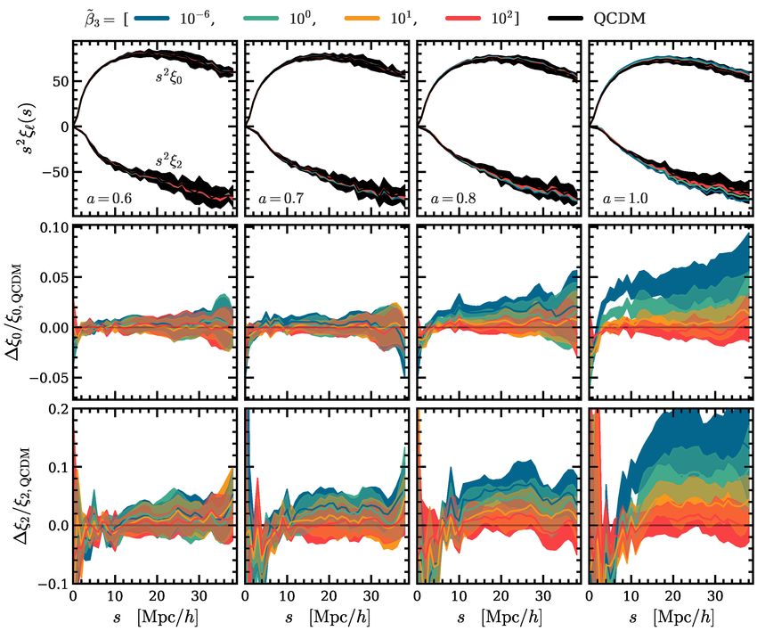
2h−1 Mpc due to the halo exclusion effect. We show their respective 2PCFs in the top row of
figure 7 for a = 0.6 (outer left), a = 0.7 (inner left), a = 0.8 (inner right) and a = 1.0 (outer
right). As expected, the 2PCFs drop off with halo separation, and can be well described by
a power law across the entire range of scales probed here.
– 18 –You can also read