Radiation reaction in electron-beam interactions with high-intensity lasers - arXiv.org
←
→
Page content transcription
If your browser does not render page correctly, please read the page content below
Radiation reaction in electron-beam interactions with high-intensity lasers

                                                                                                  T. G. Blackburn∗
                                                             Department of Physics, University of Gothenburg, Gothenburg SE-41296, Sweden
                                                                                               (Dated: March 31, 2020)
arXiv:1910.13377v2 [physics.plasm-ph] 30 Mar 2020

                                                                                                      Abstract
                                                        Charged particles accelerated by electromagnetic fields emit radiation, which must, by the conservation
                                                    of momentum, exert a recoil on the emitting particle. The force of this recoil, known as radiation reaction,
                                                    strongly affects the dynamics of ultrarelativistic electrons in intense electromagnetic fields. Such environ-
                                                    ments are found astrophysically, e.g. in neutron star magnetospheres, and will be created in laser-matter
                                                    experiments in the next generation of high-intensity laser facilities. In many of these scenarios, the energy
                                                    of an individual photon of the radiation can be comparable to the energy of the emitting particle, which
                                                    necessitates modelling not only of radiation reaction, but quantum radiation reaction. The worldwide de-
                                                    velopment of multi-petawatt laser systems in large-scale facilities, and the expectation that they will create
                                                    focussed electromagnetic fields with unprecedented intensities > 1023 Wcm−2 , has motivated renewed in-
                                                    terest in these effects. In this paper I review theoretical and experimental progress towards understanding
                                                    radiation reaction, and quantum effects on the same, in high-intensity laser fields that are probed with ultra-
                                                    relativistic electron beams. In particular, we will discuss how analytical and numerical methods give insight
                                                    into new kinds of radiation-reaction-induced dynamics, as well as how the same physics can be explored in
                                                    experiments at currently existing laser facilities.

                                                    ∗   tom.blackburn@physics.gu.se

                                                                                                          1
CONTENTS

     I. Introduction                                                                                2

 II. Theory of radiation reaction                                                                   8
       A. Classical radiation reaction                                                              8
          1. In plane electromagnetic waves                                                         9
       B. Quantum corrections: suppression and stochasticity                                       11

III. Numerical modelling and simulations                                                           16
       A. Classical regime                                                                         16
       B. Quantum regime: the ‘semiclassical’ approach                                             18
       C. Benchmarking, extensions and open questions                                              21

IV. Experimental geometries, results and prospects                                                 24
       A. Geometries                                                                               24
       B. ‘All-optical’ colliding beams                                                            27
       C. Recent results                                                                           29

 V. Summary and outlook                                                                            33

       Acknowledgments                                                                             35

       References                                                                                  35

I.     INTRODUCTION

      It is a well-established experimental fact that charged particles, accelerating under the action
of externally imposed electromagnetic fields, emit radiation [1, 2]. The characteristics of this
radiation depend strongly upon the magnitude of the acceleration as well as the shape of the
particle trajectory. For example, if relativistic electrons are made to oscillate transversely by a
field configuration that has some characteristic frequency ω0 , they will emit radiation that has
characteristic frequency 2γ 2 ω0 , where γ is their Lorentz factor. Given ω0 corresponding to a
wavelength of one micron and an electron energy of order 100 MeV, this easily approaches the
100s of keV or multi-MeV range [3].

                                                  2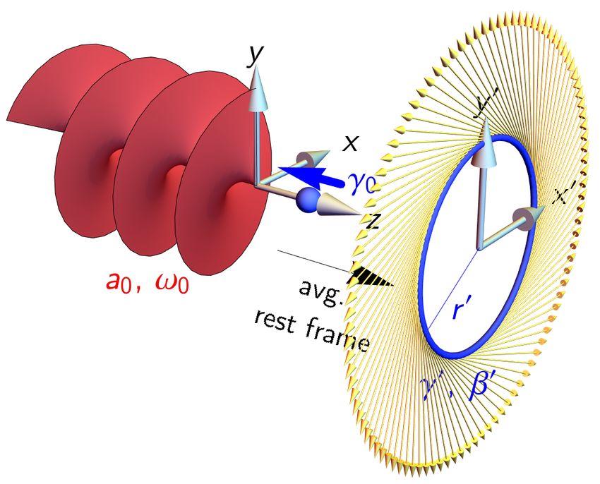
The total power radiated, as we shall see, increases strongly with γ and the magnitude of the
acceleration. We can then ask: as radiation carries energy and momentum, how do we account for
the recoil it must exert on the particle? Equivalently, how do we determine the trajectory when
one electromagnetic force acting on the particle is imposed externally and the other arises from
the particle itself? That this remains an active and interesting area of research is a testament not
only to the challenges in measuring radiation reaction effects experimentally [4], but also to the
difficulties of the theory itself [5, 6]. The ‘correct’ formulation of radiation reaction within classi-
cal electrodynamics has not yet been absolutely established, nor has the complete corresponding
theory in quantum electrodynamics. While these points are undoubtedly of fundamental interest, it
is important to note that radiation reaction and quantum effects will be unavoidable in experiments
with high-intensity lasers and therefore these questions are of immense practical interest as well.
   This is motivated by the fast-paced development of large-scale, multipetawatt laser facili-
ties [7]: today’s facilities reach focussed intensities of order 1022 Wcm−2 [8–10], and those up-
coming, such as Apollon [11], ELI-Beamlines [12] and Nuclear Physics [13], aim to reach more
than 1023 Wcm−2 , with the added capability of providing multiple laser pulses to the same target
chamber. At these intensities, radiation reaction will be comparable in magnitude to the Lorentz
force, rather than being a small correction, as is familiar from storage rings or synchrotrons. Fur-
thermore, significant quantum corrections to radiation reaction are expected [5], which profoundly
alters the nature of particle dynamics in strong fields.
   The purpose of this review is to introduce the means by which radiation reaction, and quan-
tum effects on the same, are understood, how they are incorporated into numerical simulations,
and how they can be measured in experiments. While there is now an extensive body of litera-
ture considering experimental prospects with future laser systems, our particular focus will be the
relevance to today’s high-intensity lasers. It is important to note that much of the same physics
can be explored by probing such a laser with an ultrarelativistic electron beam. Previously such
experiments demanded a large conventional accelerator [14, 15], but now ‘all-optical’ realization
of the colliding beams geometry is possible thanks to ongoing advances in laser-wakefield accel-
eration [16, 17]. Indeed, the first experiments to measure radiation-reaction effects in this config-
uration have recently been reported by Cole et al. [18], Poder et al. [19]. This review attempts to
provide the theory context for the interest in their results.
   Let us begin by introducing the various parameters that determine the importance of radiation
emission, radiation reaction, and quantum effects. We work throughout in natural units such that

                                                  3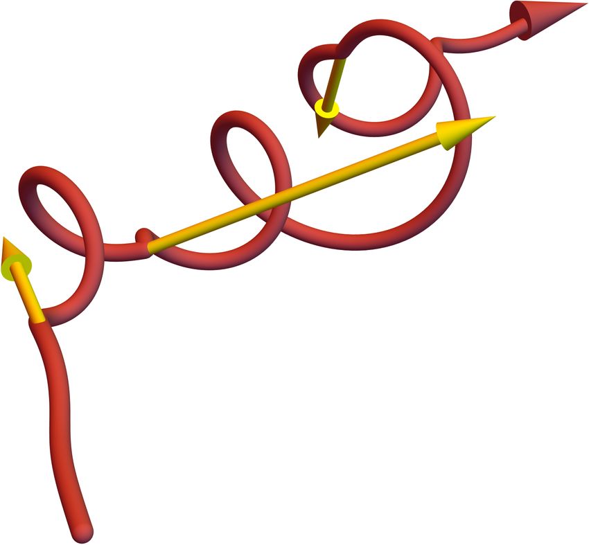
FIG. 1.    Interaction of an electron (initial Lorentz factor γ0 ) and a circularly polarized electromagnetic
wave (frequency ω0 and normalized amplitude a0 ). In its average rest frame the electron is accelerated on a
circular trajectory, with Lorentz factor γ 0 = (1 + a20 )1/2 , velocity β 0 and radius r0 . The acceleration leads to
the emission of synchrotron radiation, which has characteristic frequency ω 0 ' γ 03 /r0 .

the reduced Planck’s constant h̄, the speed of light c and the vacuum permittivity ε0 are all equal
to unity: h̄ = c = ε0 = 1. In these units the fine-structure constant α = e2 /(4π), where e is the
elementary charge.

   It will be helpful to consider the concrete example shown in fig. 1. Here an electron is ac-
celerated by a circularly polarized, monochromatic plane electromagnetic wave. The wave has
angular frequency ω0 and dimensionless amplitude a0 = eE0 /(mω0 ), where E0 is the magnitude
of the electric field and m is the electron mass. a0 is sometimes called the strength parameter or
the normalized vector potential, and it can be shown to be both Lorentz- and gauge-invariant [20].
The solution to the equations of motion, where the force is given by the Lorentz force only, can be
found in many textbooks (see Gibbon [21] for example), so we will only summarize it here.

   The electromagnetic field tensor for the wave is eFµν = ma0 ∑i fi0 (φ )(kµ ενi − kν εµi ), where k
is the wavevector, primes denote differentiation with respect to phase φ = k.x, and the ε1,2 are
constant polarization vectors that satisfy εi2 = −1 and k.εi = 0. Then the four-momentum of the

                                                        4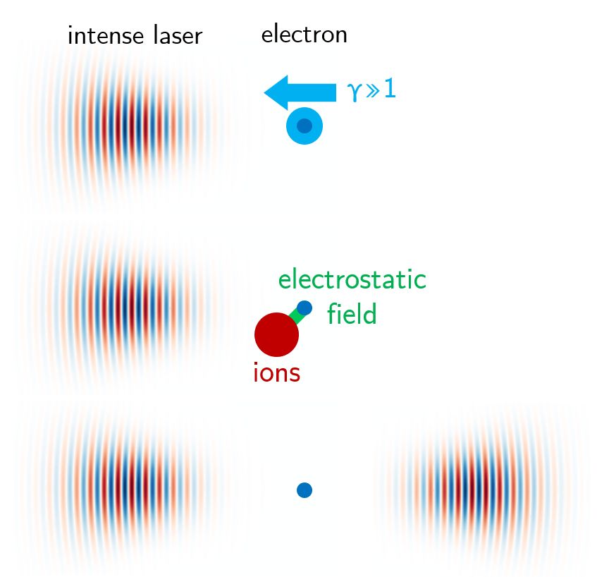
electron p may be written in terms of the potential eAµ = ma0 ∑i fi (φ )εµi :

                                                    eA.p0 e2 A2

                               µ         µ       µ
                             p (φ ) =   p0   + eA −       +         kµ .                               (1)
                                                     k.p0   2k.p0
                                                                                           R
Translational symmetry guarantees that k.p = k.p0 . The electron trajectory xµ (φ ) = (pµ /k.p) dφ .
   Let us say that the electron initially counterpropagates into a circularly polarized, monochro-
matic wave, with velocity β0 and Lorentz factor γ0 . The electron is accelerated by the wave in
the longitudinal direction, parallel to its wavevector, reaching a steady drift velocity of βd . Trans-
forming to the electron’s average rest frame (ARF), as shown in fig. 1, we find that the electron
executes circular motion with Lorentz factor γ 0 = (1 + a20 )1/2 , velocity β 0 = a0 (1 + a20 )−1/2 and
radius r0 = a0 /[γ0 (1 + β0 )ω0 ]. That γ 0 is constant tells us that there is a phase shift of π/2 between
the rotation of the velocity and electric field vectors v and E, so v · E = 0 and the external field
does no work on the charge.
   The instantaneous acceleration of the charge is non-zero so the electron emits radiation while
describing this orbit. We can use classical synchrotron theory [22] to calculate the energy radiated
in a single cycle Erad , as a fraction f of the electron energy in the ARF γ 0 m, with the result
f = Erad /(γ 0 m) = 4πRc /3. The magnitude of the radiation losses is controlled by the invariant
classical radiation reaction parameter [23]

                              αa20 γ0 (1 + β0 )ω0
                         Rc ≡                                                                          (2)
                                    m
                                          E0

                                                        I0        λ
                            ' 0.13                                    .                                (3)
                                      500 MeV      1022 Wcm−2    µm

Here E0 is the initial energy of the electron, I0 = E02 the laser intensity and λ = 2π/ω0 its wave-
length.
   If we define ‘significant’ radiation damping to be an energy loss of approximately 10% per
                                                                 1/2
period [24], we find the threshold to be Rc & 0.024, or a0 γ0          & 7 × 10² for a laser with a wave-
length of 0.8 µm. At this point the force on the electron due to radiative losses must be included
in the equations of motion. We can see this directly by comparing the magnitudes of the radiation
reaction and Lorentz forces. Estimating the former as Frad = Erad /(2πr0 ) and the Lorentz force
as Fext = γ 0 m/r0 , we have that Frad /Fext ' 2Rc /3. For Rc & 1 we enter the radiation-dominated
regime [25–27].
   We will discuss how the recoil due to radiation emission is included in classical electrodynam-
ics in section II A. Before doing so, let us also consider the spectral characteristics of the radiation

                                                     5
emitted by the accelerated electron. In principle the periodicity of the motion, and its infinite dura-
tion, means that the frequency spectrum is made up of harmonics of the ARF cyclotron frequency.
However, recall that at large γ 0 ' a0 , relativistic beaming means that most of the radiation is emit-
ted in the forward direction into a cone with half-angle 1/γ 0 . The length of the overlap between
the electron trajectory and this cone defines the formation length l f , which is the characteristic
distance over which radiation is emitted [28, 29]. A straightforward geometrical calculation gives
the ratio between l f and the circumference of the orbit C = 2πr0
lf 1
' . (4)
C 2πa0
The invariance of a0 suggests we could have reached this result in a covariant way; indeed, a full
determination of the size of the phase interval that contributes to emission gives the same result,
even quantum mechanically [30].
The smallness of the formation zone means that the spectrum is broadband, with frequency
components up to a characteristic value ω 0 ' γ 03 /r0 . Comparing this characteristic frequency to
the cyclotron frequency (in the average rest frame) ωc = 1/r0 gives us a measure of the classical
nonlinearity:
ω0
' a30 . (5)
ωc
At a0
1, the radiation is made up of very high harmonics and is therefore well-separated from the
background. The ratio between the frequency ω 0 and the electron energy in the ARF χ = ω 0 /(γ 0 m)
is another useful invariant parameter
a0 γ0 (1 + β0 )ω0
χ≡ (6)
m
1/2
E0
I0
' 0.29 . (7)
500 MeV 1022 Wcm−2
Restoring factors of h̄ and c we can show that χ ∝ h̄, unlike Rc . It therefore parametrizes the
importance of quantum effects on radiation reaction [30, 31], as can be seen by the fact that if
χ ∼ 1, an individual photon of the radiation can carry off a substantial fraction of the electron’s
energy. By setting γ0 = 1 in eq. (6), we can show that χ is equal to the ratio of the electric field in
the instantaneous rest frame of the electron to the so-called critical field of QED [32, 33]
m2
Ecr ≡ = 1.326 × 10¹⁸ Vm−1 , (8)
e
which famously marks the threshold for nonperturbative electron-positron pair creation from the
vacuum [34].
610
55 0,
Rc
Rc
eV
5
1. 00
=0
=0
0= 1
ω γ=
.0
.1
1
1
Wistisen et al. (2018)
0.50
a0
χ
γ=
Bula et al. (1996), Poder et al. (2018)
Burke et al. (1997)
0.10
0.05 Cole et al. (2018)
Wistisen et al. (2019)
0.01
0.1 1 10 100 1000
a0
FIG. 2. The importance, and type, of radiation reaction effects can be parametrized by a0 , the normalized
intensity of the laser field or classical nonlinearity parameter, and χ, the quantum nonlinearity parameter.
Classical radiation damping becomes strong when Rc = αa0 χ > 0.01 (light blue) and dominates when
Rc > 0.1 (darker blue). Quantum corrections to the spectrum become necessary when χ > 0.1. Electron-
positron pair creation and QED cascades are important for χ > 1. Experiments that have explored quantum
effects with intense lasers are shown by open circles [14, 15, 18, 19]. Two recent experiments with lepton
beams and aligned crystals are shown by triangles [35, 36]; here the perpendicular component of the lepton
momentum p⊥ is used to define an equivalent classical nonlinearity parameter a0 ' p⊥ /m.
The two parameters Rc and χ allow us to characterize the importance of classical and quantum
radiation reaction respectively. We show these as functions of a0 and χ, the classical and quantum
nonlinearity parameters, in fig. 2. It is evident that, as a0 increases, it requires less and less electron
energy to enter the radiation-dominated regime. Indeed, if the acceleration is provided entirely by
the laser so that γ ' a0 , radiation reaction becomes dominant at about the same a0 that quantum
effects become important, assuming that ω0 corresponds to a wavelength of 0.8 µm. However, for
a0 . 50 as is accessible with existing lasers [8–10], it is not possible to probe radiation reaction
via direct illumination of a plasma. Instead, the experiments illustrated in fig. 2 have used pre-
accelerated electrons to explore the strong-field regime, thereby boosting both Rc and χ. (Note
7that, as Rc is defined on a per-cycle basis, it would be possible for classical radiation reaction
effects to be large in long laser pulses while remaining below the threshold for quantum effects.)
The next generation of laser facilities will reach a0 in excess of 100, perhaps even 1000 [11–13].
The plasma dynamics explored in such experiments will be strongly affected by radiation reaction
and quantum effects.
II. THEORY OF RADIATION REACTION
A. Classical radiation reaction
In classical electrodynamics, radiation reaction is the response of a charged particle to the field
of its own radiation [37, 38]. The first equation of motion to include both the external and self-
induced electromagnetic forces in a manifestly covariant and self-consistent way was obtained
by Dirac [39]. This solution starts from the coupled Maxwell’s and Lorentz equations and fea-
tures a mass renormalization that is needed to eliminate divergences associated with a point-like
charge [40, 41]. The result is generally referred to as the Lorentz-Abraham-Dirac (LAD) equation.
For an electron with four-velocity u, charge −e and mass m it reads
e2 d2 uµ
duµ e µ duν du
ν
= − F µν uν + + u (9)
dτ m 6πm dτ 2 dτ dτ
where τ is the proper time. Here Fµν is the field tensor for the externally applied electromagnetic
field, so it is the second term that accounts for the self-force. Although the LAD equation is
an exact solution of the Maxwell-Lorentz system, using it directly turns out to be problematic.
d2 uµ
The momentum derivative dτ 2
in the RR term leads to so-called runaway solutions, in which the
electron energy increases exponentially in the absence of external fields, and to pre-acceleration,
in which the momentum changes in advance of a change in the applied field [42–44]. These issues
have prompted searches for alternative classical theories of radiation reaction [45–49] that have
more satisfactory properties (see the review by [6] for details).
The most widely used classical theory is that proposed by [50]. They realized that if the second
(RR) term in eq. (9) were much smaller than the first in the instantaneous rest frame of the charge,
du
it would be possible to reduce the order of the LAD equation by substituting dτ → me F µν uν in the
RR term. The result, called the Landau-Lifshitz equation, is first-order in the electron momentum
8and free from the pathological solutions of the LAD equation [6]:
duµ e e4 h m
− (∂α F µν )uν uα +F µν Fνα uα + (F να uα )2 uµ .
= − F µν uν + (10)
dτ m 6πm e
The following two conditions for the characteristic length scale L over which the field varies and
its magnitude E must be fulfilled in the instantaneous rest frame for the order reduction procedure
to be valid: L
λC and E
Ecr /α, where λC = 1/m is the Compton length. Note that both of
these are automatically fulfilled in the realm of classical electrodynamics [5], as quantum effects
can only be neglected when L
λC and E
Ecr . The former condition ensures that the electron
wavefunction is well-localized and the latter means recoil at the level of the individual photon is
negligible [5]. One reason to favour the Landau-Lifshitz equation is that all physical solutions of
the LAD equation are solutions of the Landau-Lifshitz equation [51].
Once the trajectories are determined, the self-consistent radiation is obtained from the Liénard-
Wiechert potentials, which give the electric and magnetic fields of a charge in arbitrary mo-
tion [52]. The spectral intensity of the radiation from an ensemble of Ne electrons, the energy
radiated per unit frequency ω and solid angle Ω, is given in the far field by
2
d2 E αω 2 Ne Z ∞
iω(t−n·rk )
= ∑ n × (n × vk )e dt (11)
dωdΩ 4π 2 k=1 −∞
where n the observation direction, and rk and vk are the position and velocity of the kth particle at
time t [52].
1. In plane electromagnetic waves
Among the other useful properties of eq. (10) is that it can be solved exactly if the external field
is a plane electromagnetic wave [53]. Taking this field to be eFµν = ma0 ∑i fi0 (φ )(kµ ενi − kν εµi ),
using the same definitions as in section I, eq. (10) is most conveniently expressed in terms of the
lightfront momentum u− ≡ k.p/(mω0 ), scaled perpendicular momenta ũx,y ≡ ux,y /u− , and phase
φ:
du− 2αa20 ω0 0 2 2
=− [ f1 (φ ) + f20 (φ )2 ]u− , (12)
dφ 3m
and
dũi a0 fi0 (φ ) 2αa0 ω0 fi00 (φ )
= + . (13)
dφ u− 3m
9The remaining component u+ is determined by the mass-shell condition u− u+ − u2x − u2y = 1 and
µ /u− ) dφ .
Rφ
the position by integration of ω0 xµ (φ ) = −∞ (u Equation (12) admits the solution
u−
u− = 0
, (14)
1 + 32 Rc I(φ )
where u−
0 is the initial lightfront momentum, the classical radiation reaction parameter Rc =
a20 u− 0 0
Rφ 2 2
0 ω0 /m as in eq. (2), and I(φ ) = −∞ [ f 1 (ψ) + f 2 (ψ) ] dψ. The choice of notation here re-
flects the fact that f 0 (φ ) is proportional to the electric field and so I(φ ) is like an integrated energy
flux. We use eq. (14) to solve eq. (13), obtaining ũi (φ ) and then
1 2Rc 2Rc 0
ui = ui,0 + a0 fi (φ ) + H(φ ) + f (φ ) , (15)
1 + 23 Rc I(φ ) 3 3a0 i
0
Rφ
where ui,0 is the initial value of the perpendicular momentum component i and Hi (φ ) = −∞ f i (ψ)I(ψ) dψ.
The electron trajectory in the absence of radiation reaction is obtained by setting α = 0, in which
case we recover eq. (1) as expected. Note that the lightfront momentum u− is no longer conserved,
once radiation reaction is taken into account [54].
In section I we estimated that the electron would radiate in a single cycle a fraction 4πRc /3
of its total energy. Using our analytical result eq. (14) and assuming γ
1 so that u− ' 2γ, we
can show this fraction is actually Erad /(γ0 m) = (4πRc /3)/(1 + 4πRc /3). Here the denominator
represents radiation-reaction corrections to the energy loss, guaranteeing that Erad /(γ0 m) < 1. With
these corrections, the energy emitted, according to the Larmor formula, is equal to the energy
lost, according to the Landau-Lifshitz equation (see Appendix A of Di Piazza [55] for a direct
calculation of momentum conservation).
The emission spectrum eq. (11) may also be expressed in terms of an integral over phase. The
number of photons scattered per unit (scaled) frequency s = ω/ω0 and solid angle is [56, 57]
2
d2 Nγ αs Ne Z ∞
ε 0 .uk exp(−isn.ξk )
= 2 ∑ dφ (16)
dsdΩ 4π k=1 −∞ (u−
k)
2
where the scaled four-position ξ ≡ ω0 x, and ε 0 and n are the four-polarization and propagation
direction of the scattered photon. Given these relations and the analytically determined trajectory,
we can numerically evaluate the number of photons scattered to given frequency and polar angle
by integrating eq. (16), summed over polarizations, over all azimuthal angles 0 ≤ ϕ < 2π.
10B. Quantum corrections: suppression and stochasticity
We showed in fig. 2 that in many scenarios of interest, reaching the regime where radiation
reaction becomes important automatically makes quantum effects important as well. This raises
the question: what is the quantum picture of radiation reaction? Let us revisit the example we
studied classically in section I, that of an electron emitting radiation under acceleration by a strong
electromagnetic wave. One might instinctively liken this scenario to inverse Compton scattering,
as energy and momentum are automatically conserved when the electron absorbs a photon (or
photons) from the plane wave and emits another, higher energy photon. However, the recoil is
proportional to h̄ and vanishes in the classical limit; we would then recover Thomson scattering
rather than radiation reaction.
The solution is that, in the regime a0
1 and χ . 1, quantum radiation reaction can be iden-
tified with the recoil on the electron due its emission of multiple, incoherent photons [23]. These
conditions express the following: a0
1 means that the formation length is much smaller than
the wavelength of the external field, by eq. (4), so the coherent contribution is suppressed; and
χ . 1 means pair creation can be neglected. The latter is important because QED is inherently a
many-body theory and it is possible for the final state to contain many more electrons than the ini-
tial state. As the number of photons Nγ ∝ α ∝ 1/h̄ and the momentum change of the electron ∝ h̄
for each photon, we have that the total momentum change ∝ h̄0 and therefore a classical limit ex-
ists [5]. This suggests that one way to determine the ‘correct’ theory of classical radiation reaction
is to start with a QED result and take the limit h̄ → 0. This has been accomplished for both the mo-
mentum change [58, 59] and the position [60]. In particular, Ilderton and Torgrimsson [60] were
able to show that, to first order in α, only the LAD, Landau-Lifshitz and Eliezer-Ford-O’Connell
formulations of radiation reaction were consistent with QED.
In both the classical and quantum regimes, the force of radiation reaction is directed antiparallel
to the electron’s instantaneous momentum, and its magnitude depends on the parameter χ. We
defined this earlier for the particular case of an electron in an electromagnetic wave [see eq. (6)].
In a general electromagnetic field Fµν ,
q
−(Fµν pν )2 γ
q
χ= = (E + v × B)2 − (v · E)2 , (17)
mEcr Ecr
where p = γm(1, v) is the electron four-momentum. χ depends on the instantaneous transverse
acceleration induced by the external field: in a plane EM wave, where E and B have the same
11magnitude and are perpendicular to each other, χ = γ |E| (1 − cos θ )/Ecr , where θ is the angle
between the electron momentum and the laser wavevector, and it is therefore largest in counter-
propagation. A curious consequence of eq. (17) is the existence of a radiation-free direction: no
matter the configuration of E and B, there exists a particular v that makes χ vanish [61]. Electrons
in extremely strong fields tend to align themselves with this direction, any transverse momentum
they have being rapidly radiated away [61]. As this direction is determined purely by the fields, the
self-consistent evolutions of particles and fields is determined by hydrodynamic equations [62].
The larger the value of χ, the greater the differences between the quantum and classical predic-
tions of radiation emission. Classically there is no upper limit on the frequency spectrum, whereas
in the quantum theory there appears a cutoff that guarantees ω < γm. Besides this cutoff, spin-
flip transitions enhance the spectrum at high energy [63]. Let us work in the synchrotron limit,
wherein the field may be considered constant over the formation length (i.e. l f
λ , using eq. (4)).
The classical emission spectrum, the energy radiated per unit frequency ω = xγm and time by an
electron with quantum parameter χ and Lorentz factor γ, is
dPcl 2x
Z ∞
αω
=√ 2K2/3 (ξ ) − K1/3 (y) dy , ξ= . (18)
dω 3πγ 2 ξ 3χ
Two quantum corrections emerge when χ is no longer much smaller than one: the non-negligible
recoil of an individual photon means that the spectrum has a cutoff at x = 1; and the spin con-
tribution to the radiation must be included. The former can be included directly by modifying
ξ = 2x/(3χ) → 2x/[3χ(1−x)] in eq. (18), which yields the spectrum of a spinless electron (shown
in orange in fig. 3). A neat exposition of this simple substitution is given by Lindhard [64] in
terms of the correspondence principle (see also Sørensen [65]). Then when the spin contribution
is added, we obtain the full QED result [30, 31, 66]
dPq 1 2x
Z ∞
αω
=√ 1−x+ K2/3 (ξ ) − K1/3 (y) dy , ξ= , (19)
dω 3πγ 2 1−x ξ 3χ(1 − x)
where we quote the spin-averaged and polarization-summed result. This is shown in blue in fig. 3.
dNγ dPq
The number spectrum dω = ω −1 dω (χ, γ) has an integrable singularity ∝ ω −2/3 in the limit
R dNγ
ω → 0. The total number of photons Nγ = dω dω is finite.
The combined effect of these corrections is to reduce the instantaneous power radiated by an
12×10-3
1.0 1
classical
0.8
classical 0.1
1.0
γd/dω
0.6 (cutoff-
g(χ)
corrected)
0.4 QED 0.5
10-2
0.2 0.0
0.001 1
0.0 10-3
0.0 0.5 1.0 1.5 2.0 10-3 10-2 0.1 1 10 100
ω/(γm) χ
FIG. 3. (left) Quantum corrections to the emission spectrum dP/dω at χ = 1: the classical [eq. (18)] and
quantum-corrected spectra [eq. (19)]. (right) These corrections cause the total radiated power to be reduced
by a factor g(χ): the full result (blue) and limiting expressions (black, dashed).
electron. This reduction is quantified by the factor g(χ) = Pq /Pcl , which takes the form [22, 31]
√ Z " #
9 3 ∞ 2u2 K5/3 (u) 36χ 2 u3 K2/3 (u)
g(χ) = + du (20)
8π 0 (2 + 3χu)2 (2 + 3χu)4
√
1 − 55 3 χ + 48χ 2 χ
1
16
= (21)
16Γ(2/3)
χ −4/3 χ
1
31/3 27
where K is a modified Bessel function of the second kind and Γ(2/3) ' 1.354. The limiting
expressions given in eq. (21) are within 5% of the full result for χ < 0.05 and χ > 200 respectively.
A simple analytical approximation to eq. (20) that is accurate to 2% for arbitrary χ is g(χ) '
[1 + 4.8(1 + χ) ln(1 + 1.7χ) + 2.44χ 2 ]−2/3 [66]. The changes to the classical radiation spectrum
and the magnitude of g(χ) are shown in fig. 3. Note that the total power Pq = 2αm2 χ 2 g(χ)/3
always increases with increasing χ. g(χ) is sometimes referred to as the ‘Gaunt factor’ [67],
as it is a multiplicative (quantum) correction to a classical result, first derived in the context of
absorption [68].
Figure 3 shows that the radiated power at χ ∼ 1 is less than 20% of its classically predicted
value. While this suppression does have a marked effect on the particle dynamics, it is not the
only quantum effect. As is discussed in section I, χ is the ratio between the energies of the
typical photon and the emitting electron. When this approaches unity, even a single emission
can carry off a large fraction of the electron energy, and the concept of a continuously radiating
13FIG. 4. In the classical picture, radiation reaction is a continuous drag force that arises from the emission of
very many photons that individually have vanishingly low energies (left). In the quantum regime, however,
the electrons emits a finite number of photons, any or all of which can exert a significant recoil on the
electron. The probabilistic nature of emission leads to radically altered electron dynamics, with implications
for laser-matter interactions beyond the current intensity frontier. From Blackburn [70].
particle breaks down. Instead, electrons lose energy probabilistically, in discrete portions. The
importance of this discreteness may be estimated by comparing the typical time interval between
emissions, ∆t = hωi/P, with the timescale of the laser field 1/ω0 [69]. Equation (19) yields for
the average photon energy hωi ' 0.429 χγm for χ
1 and 0.25 γm for χ
1; the radiated power
P = 2αm2 χ 2 g(χ)/3. We find
44 a−1
χ
1
0
ω0 ∆t ' . (22)
58 [γω0 /(a0 m)]1/3
χ
1
We expect stochastic effects to be at their most significant when ω0 ∆t & 1, which implies that the
total number of emissions in an interaction is relatively small but χ is large.
A description of how stochastic energy losses can be modelled follows in section III B. For now,
it suffices to interpret eq. (19) as the (energy-weighted) probability distribution of the photons
emitted at a particular instant of time. Even though two electrons may have the same χ and
γ, they can emit photons of different energies (or none at all) and thereby experience different
recoils. Contrast this with the classical picture, in which the continuous energy loss is driven by
the emission of many photons that individually have vanishingly small energies (see fig. 4).
Consider, for example, the interaction of a beam of electrons with a plane electromagnetic
dNe
wave, where the Lorentz factors of the electrons are distributed γ ∼ dγ . The distribution is
14characterized by a mean µ ≡ hγi and variance σ 2 ≡ hγ 2 i − µ 2 . Under classical radiation reac-
tion, higher energy electrons are guaranteed to radiate more than their lower energy counterparts
(P ∝ γ 2 ), with the result that both the mean and the variance of γ decrease over the course of the
interaction [71]. This is still the case if the radiated power is reduced by the Gaunt factor g(χ),
i.e. a ‘modified classical’ model is assumed (see section III A), because radiation losses remain
deterministic [72].
Under quantum radiation reaction, radiation losses are inherently probabilistic. While µ will
still decrease (more energetic electrons radiate more energy on average), the width of the distri-
bution σ 2 can actually grow [71, 73]. Ridgers et al. [67] derive the following equations for the
temporal evolution of these quantities, under quantum radiation reaction:
dµ 2αm 2
=− hχ g(χ)i (23)
dt 3
dσ 2 4αm 55αm
=− h(γ − µ)χ 2 g(χ)i + √ hγ χ 3 g2 (χ)i, (24)
dt 3 24 3
R R
where h· · ·i denotes the population average and g2 (χ) = χ dPq / χ dPcl is the second moment
of the emission spectrum. Only the first term of eq. (24) is non-zero in the classical limit, and it
is guaranteed to be negative. The second term represents stochastic effects and is always positive.
Broadly speaking, the latter is dominant if χ is large, the interaction is short, or the initial variance
is small [67, 74]. The evolution of higher order moments, such as the skewness of the distribution,
are considered in Niel et al. [74].
A distinct consequence of stochasticity is straggling [75], where an electron that radiates less
(or no) energy than expected enters regions of phase space that would otherwise be forbidden.
Unlike stochastic broadening, which can occur in a static, homogeneous electromagnetic field,
straggling requires the field to have some non-trivial spatiotemporal structure. If an unusually
long interval passes between emissions, an electron may be accelerated to a higher energy or
sample the fields at locations other than those along the classical trajectory [76]. In a laser pulse
with a temporal envelope, for example, electrons that traverse the intensity ramp without radiating
reach larger values of χ than would be possible under continuous radiation reaction; this enhances
high-energy photon production and electron-positron pair creation [77]. If the laser duration is
short enough, it is probable that the electron passes through the pulse without emitting at all, in
so-called quenching of radiation losses [78].
The quantum effects we have discussed in this section emerge, in principle, from analytical re-
sults including the emission spectrum [eq. (19)]. While further analytical progress can be made in
15the quantum regime, using the theory of strong-field QED (see section III B), modelling more re-
alistic laser–electron-beam or laser-plasma interactions generally requires numerical simulations.
Much effort has been devoted to the development, improvement, benchmarking and deployment of
such simulation tools over the last few years. In the following section we review these continuing
developments.
III. NUMERICAL MODELLING AND SIMULATIONS
A. Classical regime
A natural starting point is the modelling of classical radiation reaction effects. In the absence
of quantum corrections, we have all the ingredients we need to formulate a self-consistent picture
of radiation emission and radiation reaction. We showed in section I how using only the Lorentz
force to determine the charge’s motion and therefore its emission led to an inconsistency in energy
balance. This is remedied by using either eq. (9) or eq. (10) as the equation of motion, in which
case the energy carried away in radiation matches that which is lost by the electron.
Implementations of classical radiation reaction in plasma simulation codes have largely favoured
the Landau-Lifshitz equation (or a high-energy approximation thereto), as it is first-order in the
momentum and the additional computational cost is not large [54, 79–81]. These codes have not
only been used to study radiation reaction effects in laser-plasma interactions [72, 82–86], but
also whether there are observable differences between models of the same [87, 88]. The radiation
reaction force proposed by Sokolov [49] has also been implemented in some codes [89, 90], but
note that it is not consistent with the classical limit of QED [60]. It is also possible to solve the
LAD equation numerically via integration backward in time [91].
Given data on the trajectories of an ensemble of electrons (usually a subset of the all electrons
in the simulations), eq. (11) can be used to obtain the far-field spectrum in a simulation where
classical radiation reaction effects are included [24, 92, 93]. Equation (11) is valid across the
full range of ω (pace the quantum cutoff at ω = γm), including the low-frequency region of the
1/3
spectrum where collective effects are important: ω < ne , where ne is the electron number density.
This region does not, however, contribute very much to radiation reaction; this is dominated by
1/3
photons near the synchrotron critical energy ωc
ne . Thus the spectrum can be divided into
coherent and incoherent parts, that are well separated in terms of their energy [69]. In the latter
16region, the order of the summation and integration in eq. (11) can be exchanged, and the total
spectrum determined by summing over the single-particle spectra.
In a particle-in-cell code for example, the electromagnetic field is defined on a grid of discrete
points and advanced self-consistently using currents that are deposited onto the same grid [94].
Defining the grid spacing to be ∆, this scheme will directly resolve electromagnetic radiation
that has a frequency less than the Nyquist frequency π/∆.1 Given appropriately high resolution,
this accounts for the coherent radiation generated by the collective dynamics of the ensemble of
particles. The recoil arising from higher frequency components, which cannot be resolved on the
grid, and in any case as a self-interaction is neglected, is accounted for by the radiation reaction
force.
Further simplification is possible if the interference of emission from different parts of the
trajectory is negligible. As indicated in section I, at high intensity a0
1, the formation length
of the radiation is much smaller than the timescale of the external field (see eq. (4)). This being
the case, rather than using eq. (11), we may integrate the local emission spectrum eq. (18) over
the particle trajectory, assuming that, at high γ, the radiation is emitted predominantly in direction
parallel to the electron’s instantaneous velocity [56, 95, 96]. The approach is naturally extended
to account for quantum effects, by substituting for the classical synchrotron spectrum eq. (18) the
equivalent result in QED, eq. (19).
One consequence of doing so is that the radiated power is reduced by the factor g(χ), given in
eq. (20). This should be reflected in a reduction in the magnitude of the radiation-reaction force.
Consequently, a straightforward, phenomenological way to model quantum radiation reaction is to
use a version of eq. (10) where the second term is scaled by g(χ). This ‘modified classical’ model
has been used in studies of laser–electron-beam [24, 72, 77] and laser-plasma interactions [97,
98] as a basis of comparison with a fully stochastic model (shortly to be introduced), as well as
in experimental data analysis [19, 35]. It has been shown that this approach yields the correct
equation of motion for the average energy of an ensemble of electrons in the quantum regime [67,
74]. It is, however, deterministic, and therefore neglects the stochastic effects we discussed in
section II B.
1 Sampling at discrete points, i.e. with limited sampling rate, means that only a certain range of frequency compo-
nents in a given waveform can be represented. The highest frequency is called the ‘Nyquist frequency’. Modes that
lie are above this are aliased to lower frequencies.
17B. Quantum regime: the ‘semiclassical’ approach
In section II B we discussed how ‘quantum radiation reaction’ could be identified with the
recoil arising from multiple, incoherent emission of photons. Indeed, if χ & 1, any or all of these
photons can exert a significant momentum change individually. Figure 2 tells us that we generally
require a0
1 to enter the quantum radiation reaction regime with lasers, which necessitates a
nonperturbative approach to the theory. This is provided by strong-field QED, which separates
the electromagnetic field into a fixed background, treated exactly, and a fluctuating part, treated
perturbatively [99]; see the reviews by Di Piazza et al. [5], Ritus [30], Heinzl [100] or a tutorial
overview by Seipt [101] which discusses photon emission in particular.
Although it is the most general and accurate approach, strong-field QED is seldom used to
model experimentally relevant configurations of laser-electron interaction [102]. In a scattering-
matrix calculation, the object is to obtain the probability of transition between asymptotic free
states; as such, complete information about the spatiotemporal structure of the background field
is required. Analytical results have only been obtained in field configurations that possess high
symmetry [103], e.g. plane EM waves [30] or static magnetic fields [31]. The assumption that the
background is fixed also means that back-reaction effects are neglected, even though it is expected
that QED cascades will cause significant depletion of energy from those background fields [104–
106]. Furthermore, the expected number of interactions per initial particle (the multiplicity) is
much greater than one in many interaction scenarios. At present, cutting-edge results are those in
which the final state contains only two additional particles, e.g. double Compton scattering [107–
110] and trident pair creation [111–115], due to the complexity of the calculations.
The need to overcome these issues has motivated the development of numerical schemes that
can model quantum processes at high multiplicity in general electromagnetic fields. In this article
we characterize these schemes as ‘semiclassical’, by virtue of the fact that they factorize a QED
process into a chain of first-order processes that occur in vanishingly small regions linked by
classically determined trajectories, as illustrated in fig. 5. The rates and spectra for the individual
interactions are calculated for the equivalent interaction in a constant, crossed field, which may
be generalized to an arbitrary field configuration under certain conditions. The first key result
is that, at a0
1, the formation length of a photon (or an electron-positron pair) is much smaller
than the length scale over which the background field varies (see section I) and so emission may be
treated as occurring instantaneously [30]. The second is that if χ 2
|F| , |g| and F2 , g2
1, where
182
γ(k1 )γ(k )
2
e− (p− )
PQED
e− →e− e− e+ γγ ∝ e− (pi )
e+ (p+ )
e− (pf )
is simulated as
dpµ e
dτ =m Fµν pν
∂µ F µν = j ν
p+
k1
p−
k2
p 2
k3
p0
2 PCCF
γ→e+ e− [χ(t4 )]
p1 2
pi dkµ
p2
dτ =0
p01
PCCF
e→eγ [χ(t1 )]
p02 2
PCCF
e→eγ [χ(t 2 )] p3
dpµ e p03
dτ = −m Fµν pν Pe→eγ [χ(t3 )]
CCF
∂µ F µν = j ν
pf
external field Fµν
FIG. 5. A general strong-field QED interaction, featuring the emission and creation of multiple photons and
electron-positron pairs, is simulated ‘semiclassically’ by breaking it down into a chain of first-order pro-
cesses (electrons, photons and positrons in blue, orange and red, respectively). Between these pointlike, in-
stantaneous events, the particles follow classical trajectories guided by the Lorentz force: ṗµ = ±eFµν pν /m
and Ẋ µ = pµ /m, dots denoting differentiation with respect to proper time τ. Modification of the external
field Fµν is driven by the classical currents j µ (x) = ±(e/m) pµ (τ)δ 4 [x − X(τ)] dτ. The probability rates
R
and spectra for the first-order processes are those for a constant, crossed field, and depend on the local value
of the quantum parameter χ(t) = Fµν [X(t)]pν (t) /(mEcr ).
19F = (E2 − B2 )/Ecr
2 and g = E · B/E 2 are the two field invariants, the probability of a QED process
cr
is well approximated by its value in a constant, crossed field: P(χ, F, g) ' P(χ, 0, 0)+O(F)+O(g)
[see Appendix B of Baier et al. [66]]. The combination of the two is called the locally constant,
crossed field approximation (LCFA). The first requires the laser intensity to be large, whereas the
second requires the particle to be ultrarelativistic and the background to be weak (as compared
to the critical field of QED). We will discuss the validity of these approximations, and efforts to
benchmark them, in section III C.
Within this framework, the laser-beam (or laser-plasma) interaction is essentially treated clas-
sically, and quantum interactions such as high-energy photon emission added by hand. The evo-
lution of the electron distribution function F = F (t, r, p), including the classical effect of the
background field and stochastic photon emission, is given by [67, 116]
∂F p ∂F p×B ∂F
+ · −e E+ ·
∂t γm ∂ r γm ∂p
Z Z
0 3 0
= −F Wγ (p, k ) d k + F (p0 )Wγ (p0 , p0 − p) d3 p0 , (25)
where Wγ (p, k0 ) is the probability rate for an electron with momentum p to emit a photon with
momentum k0 . A direct approach to kinetic equations of this kind is to solve them numeri-
cally [71, 117, 118], or reduce them by means of a Fokker-Planck expansion in the limit χ
1 [74]. However, the most popular is a Monte Carlo implementation of the emission operator
[the right hand side of eq. (25)], which naturally extends single-particle or particle-in-cell codes
that solve for the classical evolution of the distribution function in the presence of externally pre-
scribed, or self-consistent, electromagnetic fields [76, 116]. This method is discussed in detail in
Gonoskov et al. [69], Ridgers et al. [119], so we only summarize it here for photon emission.
The electron distribution function is represented by an ensemble of macroparticles, which rep-
resent a large number w of real particles (w is often called the weight). The trajectory of a macro-
electron between discrete emission events is determined solely by the Lorentz force. Each is
assigned an optical depth against emission T = − log(1 − R) for pseudorandom 0 ≤ R < 1, which
dT
evolves as dt = −Wγ , where Wγ is the probability rate of emission, until the point where it falls
below zero. Emission is deemed to occur instantaneously at this point and T is reset. The en-
ergy of the photon ω 0 = |k0 | is pseudorandomly sampled from the quantum emission spectrum
dNγ dPq
dω = ω −1 dω (χ, γ) [see eq. (19)] and the electron recoil determined by the conservation of mo-
mentum p = p0 + k0 and the assumption that k0 k p if γ
1. If desired, a macrophoton with the
same weight as the emitting macroelectron can be added to the simulation. Electron-positron pair
20creation by photons in strong electromagnetic fields is modelled in an analogous way to photon
emission [69, 119].
Thus there are two distinct descriptions of the electromagnetic field. One component is treated
as a classical field (in a PIC code, this would be discretized on the simulation grid) and the other
as a set of particles. In principle this leads to double-counting; however, as we discussed in
section III A, the former lies at much lower frequency than the photons that make up synchrotron
emission, and has a distinct origin in the form of externally generated fields (such as a laser pulse)
or the collective motion of a plasma. Coherent effects are much less important for the high-
frequency components, which justifies describing them as particles [69].
C. Benchmarking, extensions and open questions
The validity of the simulation approach discussed in section III B relies on the assumption that
a high-order QED process in a strong electromagnetic background field may be factorized into a
chain of first-order processes, each of which is well approximated by the equivalent process in a
constant, crossed field. It is generally expected that this reduction works in scenarios where a0
1
and χ 2
|F| , |g| [30, 66]. However, these asymptotic conditions do not give quantitative bounds
on the error made by semiclassical simulations. As these are the primary tool by which we predict
radiation reaction effects in high-intensity lasers, it is important that they are benchmarked and
that the approximations are examined.
One approach is to compare, directly, the predictions of strong-field QED and simulations. We
focus here on results for single nonlinear Compton scattering [102, 120, 121], the emission of one
and only one photon in the interaction of an electron with an intense, pulsed plane EM wave, by
virtue of its close relation to radiation reaction. It is shown that the condition a0
1 is necessary,
but not sufficient, for the applicability of the LCFA: we also require that a30 /χ
1 for interference
effects to be suppressed [122]. These interference effects are manifest in the low-energy part of
the photon emission spectrum x = ω 0 /(γm) < χ/a30 , as the formation length for such photons is
comparable in size to the wavelength of the background field. Semiclassical simulations strongly
overestimate the number of photons emitted in this part of the spectrum because they exclude
nonlocal effects [120, 121]. Nevertheless, they are much more accurate with respect to the total
energy loss (and therefore to radiation reaction), because this depends on the power spectrum,
to which the low-energy photons do not contribute significantly [102]. This is shown in fig. 6,
21300 0.25
0.20 a0=10
200
k- dNγ/dk-
0.15 a0=5
Δp-/m
exact QED
0.10
100
simulations 0.05
0 0.00
5 10 15 20 25 30 10-5 10-4 10-3 10-2 0.1 1
a0 k-/p-
FIG. 6. Comparison between exact QED (grey) and simulation results (blue and orange) for single non-
linear Compton scattering of an electron in a two-cycle, circularly polarized laser pulse: (left) the lightfront
momentum loss as a function of laser amplitude a0 ; and (right) exemplary photon spectra. Adapted from
Blackburn et al. [102].
which compares the predictions of exact QED and semiclassical simulations for an electron with
p−
0 /m ' 2γ0 = 2000 colliding with a two-cycle laser pulse with normalized amplitude a0 and
wavelength λ = 0.8 µm. There is remarkably good agreement between the two even for a0 = 5.
An additional point of comparison in Blackburn et al. [102] is the number of photons absorbed
from the background field in the process of emitting a high-energy photon. This transfer of energy
from the background field to the electron is required by momentum conservation. Without emis-
sion, there would be no such transfer of energy. This is consistent with the classical picture, in
which plane waves do no work in the absence of radiation reaction. Strong-field QED calculations
depend crucially on the fixed nature of the background field; however, for single nonlinear Comp-
ton scattering, near-total depletion of the field is predicted at a0 & 1000 [123]. The theory must
therefore allow for changes to the background [124]. Within the semiclassical approach, depletion
is accounted for by the action of the classical currents through the j · E term in Poynting’s theorem.
Quantum effects are manifest in how photon emission (and pair creation), modify those classical
currents, as illustrated in fig. 5. In Blackburn et al. [102], the classical work done on the elec-
tron is shown to agree well with the number of absorbed photons predicted by exact QED. This
is consistent with the results of Meuren et al. [125], which indicate that the ‘classical’ dominates
the ‘quantum’ component of depletion, the latter associated with absorption over the formation
length, if a0
1.
22The failure of the semiclassical approach to reproduce the low-energy part of the photon
dNγ
spectrum arises from the localization of emission. Most notably, the number spectrum dω =
dPq
ω −1 dω (χ, γ) [see eq. (19)] diverges as ω −2/3 as ω → 0. This can be partially ameliorated
by the use of emission rates that take nonlocal effects into account. Di Piazza et al. [126] sug-
gest replacing the LCFA spectrum in the region x . χ/a30 with the equivalent, finite, result for a
monochromatic plane wave, which they adapt for use in arbitrary electromagnetic field configura-
tions. Ilderton et al. [127] propose an approach based on formal corrections to the LCFA, in which
the emission rates depend on the field gradients as well as magnitudes.
While the studies discussed above have given insight into the limitations of the LCFA, they do
not examine the applicability of the factorization shown in fig. 5, as this requires by definition the
calculation of a higher order QED process. At the time of writing, there are no direct comparisons
of semiclassical simulations and strong-field QED for either double Compton scattering (emission
of two photons) or trident pair creation (emission of a photon which decays into an electron-
positron pair). Factorization, also called the cascade approximation, has been examined directly
within strong-field QED for the trident process in a constant crossed field [113] and in a pulsed
plane wave [114, 115]. In the latter it is shown that at a0 = 50 and an electron energy of 5 GeV,
the error is approximately one part in a thousand.
The dominance of the cascade contribution makes it important to consider whether the propa-
gation of the electron between individual tree-level process, as shown in fig. 5, is done accurately.
In the standard implementation, this is done by solving a classical equation of motion including
only the Lorentz force [69, 119]. The evolution of the electron’s spin is usually neglected and
emission calculated using unpolarized rates, such as eq. (19). King [109] show that the accuracy
of modelling double Compton scattering in a constant crossed field as two sequential emissions
with unpolarized rates is better than a few per cent. There are, however, scenarios, where the
spin degree of freedom influences the dynamics to a larger degree. Modelling these interactions
with semiclassical simulations requires spin-resolved emission rates [22, 128] and an equation of
motion for the electron spin [129, 130]. In a rotating electric field, as found at the magnetic node
of an electromagnetic standing wave [104], where the spin does not precess between emissions,
the asymmetric probability of emission between different spin states leads to rapid, near-complete
polarization of the electron population [131, 132]. Similarly, an electron beam interacting with
a linearly polarized laser pulse can acquire a polarization of a few per cent [128]. To make this
larger, it is necessary to break the symmetry in the field oscillations, which can be accomplished by
23introducing a small ellipticity to the pulse [133], or by superposition of a second colour [134–136].
A more fundamental limitation on the applicability of the LCFA is that the emission rates are
calculated at tree level only. The importance of loop corrections to the strong-field QED vertex
grows as α χ 2/3 in a constant, crossed field [137], leading to speculation that α χ 2/3 is the ‘true’
expansion parameter of strong-field QED [138]. When χ ' 1600, this parameter becomes of
order unity and the meaning of a perturbative expansion in the dynamical electromagnetic field
breaks down. The recent review by Fedotov [139] has prompted renewed interest in this regime;
recent calculations of the one-loop polarization and mass operators [140] and photon emission and
helicity flip [141] in a general plane-wave background have confirmed that the power-law scaling
of radiative corrections pertains strictly to the high-intensity limit a30 /χ
1. In the high-energy
limit, radiative corrections grow logarithmically, as in ordinary (i.e., non-strong-field) QED [140,
141].
The difficulty in probing the regime α χ 2/3 & 1 is the associated strength of radiative energy
losses, which suppress γ and so χ [139]. Overcoming this barrier at the desired χ requires the
interaction duration to be very short. The beam-beam geometry proposed by Yakimenko et al.
[142] exploits the Lorentz contraction of the Coulomb field of a compressed (100 nm), ultrarel-
ativistic (100 GeV) electron beam, which is probed by another beam of the same energy. In the
laser-electron-beam scenario considered by Blackburn et al. [143], collisions at oblique incidence
are proposed for reaching χ & 100, exploiting the fact that the diameter of a laser focal spot is
typically much smaller than the duration of its temporal profile. Even higher χ is reached in the
combined laser-plasma, laser-beam interaction proposed by Baumann and Pukhov [144]. While
it seems possible to approach the fully nonperturbative regime experimentally, albeit for extreme
collision parameters, there is no suitable theory at α χ 2/3 & 1, and quantitative predictions are
lacking in this area.
IV. EXPERIMENTAL GEOMETRIES, RESULTS AND PROSPECTS
A. Geometries
It may be appreciated that the radiation-reaction and quantum effects under consideration here,
as particle-driven processes, can only become important if electrons or positrons are actually em-
bedded within electromagnetic fields of suitable strength. However, the estimates in section I were
24You can also read


