The Global Warming Time Bomb?

Can we defuse
The Global Warming Time Bomb?
All glaciers in Glacier National Park are retreating inexorably
to their final demise. Global warming is real, and the melting
ice is an apt portent of potentially disastrous consequences.
Yet most gloom-and-doom climate scenarios exaggerate trends
of the agents that drive global warming. Study of these forcing
agents shows that global warming can be slowed, and stopped,
with practical actions that yield a cleaner, healthier
atmosphere.

Figure 1. Wind and tides mix the ocean to great depths. Thus, because of the thermal inertia of this
ocean water, it requires at least several decades for the ocean temperature to respond fully to a climate
forcing.

                                                   1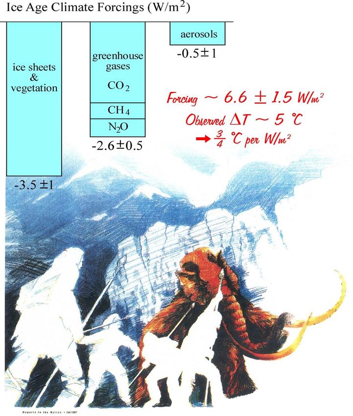

A paradox in the notion of human-made global warming became strikingly apparent to me one
summer afternoon in 1976 on Jones Beach, Long Island. Arriving at midday, my wife, son and I
found a spot near the water to avoid the scorching hot sand. As the sun sank in the late afternoon,
a brisk wind from the ocean whipped up whitecaps. My son and I had goose bumps as we ran
along the foamy shoreline and watched the churning waves.
        It was well known by then that human-made "greenhouse gases," especially carbon
dioxide (CO2) and chlorofluorocarbons (CFCs), were accumulating in the atmosphere. These
gases are a climate "forcing," because they alter the energy budget of the planet (see Box 1).
Like a blanket, they absorb infrared (heat) radiation that would otherwise escape from the Earth's
surface and atmosphere to space.
        That same summer, Andy Lacis and I, along with other colleagues at the NASA Goddard
Institute for Space Studies, had calculated that these human-made gases were heating the Earth's
surface at a rate of almost 2 W/m2. A miniature Christmas tree bulb dissipates about 1 W,
mostly in the form of heat. So it was as if humans had placed two of these tiny bulbs over every
square meter of the Earth's surface, burning night and day.
        The paradox that this result presented was the contrast between the awesome forces of
nature and the tiny light bulbs. Surely their feeble heating could not command the wind and
waves or smooth our goose bumps. Even their imperceptible heating of the ocean surface must
be quickly dissipated to great depths, so it must take many years, perhaps centuries, for the
ultimate surface warming to be achieved (Figure 1).
        This seeming paradox in the notion of human-made global warming has now been largely
resolved through study of the history of the Earth's climate, which reveals that small forces,
maintained long enough, can cause large climate change. And, consistent with the historical
evidence, the Earth has begun to warm in recent decades, at a rate predicted by climate models
that take account of the atmospheric accumulation of human-made greenhouse gases. The
warming is having noticeable impacts as glaciers are retreating worldwide, Arctic sea ice has
thinned, and spring, defined by the cyclical behavior of organisms, the average temperature and
the breakup of winter ice, comes about one week earlier than when I grew up in the 1950s.
       Yet many issues remain unresolved. How much will climate change in coming decades?
What will be the practical consequences? What, if anything, should we do about it? The debate
over these questions is highly charged because of the economic stakes inherent in any attempts to
slow the warming.
        Objective analysis of global warming requires quantitative knowledge of (1) the
sensitivity of the climate system to forcings, (2) the forcings that humans are introducing, and (3)
the time required for climate to respond. All of these issues can be studied with global climate
models, which are numerical simulations on computers. But our most accurate knowledge about
climate sensitivity, at least so far, is based on empirical data from the Earth's history.

                                                 2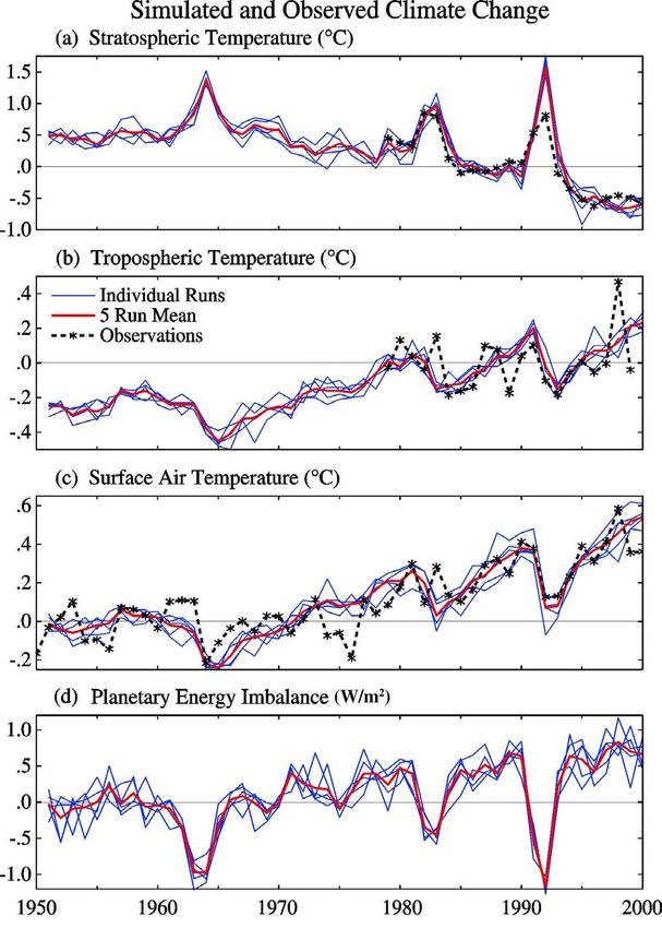

The Lessons of History
Over the past few million years the Earth’s climate has swung repeatedly between ice ages and
warm interglacial periods. Twenty thousand years ago an ice sheet covered Canada, reaching as
far south as Seattle, Iowa and New York City. More than a mile thick, the ice sheet, should it
return, would tower over and crush to dust the tallest buildings in its path.
        A 400,000 year record of temperature is preserved in the Antarctic ice sheet, which,
except for coastal fringes, escaped melting even in the warmest interglacial periods. H2O
isotopes (deuterium and 18O) in the annual snow layers reveal the temperature at which the snow
formed. This record (Figure 2) suggests that the present interglacial period (the Holocene), now
about 12,000 years old, is already long of tooth. Absent humans, the Earth might “soon” (in
thousands of years) be headed into its next ice age.The next ice age will never come, however,
unless humans desert the planet. As we shall see, the small forces that drove millennial climate
changes are now overwhelmed by human forcings. A small fraction of the gases that civilization
emits is sufficient to avert global cooling. The problem is now the opposite: human forcings are
driving the planet toward a warmer climate. Our best guide for how much the Earth’s climate
will change is provided by the record of how the Earth responded to past forcings.
        The natural millennial climate changes are associated with slow variations of the Earth’s
orbit induced by gravitational torque by other planets, mainly Jupiter and Saturn (because they
are so heavy) and Venus (because it comes so close). These torques cause the Earth’s spin axis,
now tilted 23 degrees from perpendicular to the plane of the Earth’s orbit, to wobble more than
one degree (about 40,000 year periodicity), the season at which the Earth is closest to the sun to
move slowly through the year (about 20,000 year periodicity), and the Earth’s orbit to vary from
near circular to elliptical with as much as 7 percent elongation (no regular periodicity, but large
changes on 100,000 year and longer time scales).
        These perturbations hardly affect the annual mean solar energy striking the Earth, but
they alter the geographical and seasonal distribution of insolation as much as 10-20 percent. The
insolation changes, over long periods, affect the building and melting of ice sheets. Today, for
example, the Earth is nearest the sun in January and farthest away in July. This orbital
configuration increases winter atmospheric moisture and snowfall and slows summer melting in
the Northern Hemisphere, thus, other things being equal, favoring buildup of glaciers. Insolation
and climate changes also affect uptake and release of CO2 and CH4 by plants, soil and the ocean,
as shown by changes of atmospheric CO2 and CH4 that are nearly synchronous with the climate
changes (Figure 2).
        When the temperature, CO2 and CH4 curves are carefully compared, it is found that the
temperature changes usually precede the CO2 and CH4 changes, on average by 500-1000 years.
This indicates that climate change causes CO2 and CH4 changes. However, these greenhouse gas
changes are a positive feedback that contributes to the large magnitude of the climate swings.
        Climatologists are still developing a quantitative understanding of the mechanisms by
which the ocean and land release CO2 and CH4 as the Earth warms, but the paleoclimate data are
already a goldmine of information. The most critical insight that the ice age climate swings
provide is an empirical measure of climate sensitivity.

                                                 3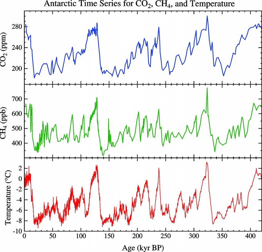

The composition of the ice age atmosphere is known precisely from air bubbles trapped
as the Antarctic and Greenland ice sheets and numerous mountain glaciers built up from annual
snowfall. The geographical distributions of the ice sheets, vegetation cover, and coastlines
during the ice age are well mapped. From these data we know that the change of climate forcing
between the ice age and today was about 6½ W/m2 (Figure 3). This forcing maintains a global
temperature change of 5°C, implying a climate sensitivity of ¾ ± ¼°C per W/m2. Climate
models yield a similar climate sensitivity. However, the empirical result is more precise and
reliable because it includes all the processes operating in the real world, even those we have not
yet been smart enough to include in the models.
        The paleo data provide another important insight. Changes of the Earth’s orbit are an
instigator of climate change, but they operate by altering atmosphere and surface properties and
thus the planetary energy balance. These atmosphere and surface properties are now influenced
more by humans than by our planet’s orbital variations. Greenhouse gases are increasing today
and glaciers and ice sheets are melting back. The old maxim, that the Earth is heading toward a
new ice age, has been rendered void by the power of modern technology.

Box 1: Climate Forcings, Sensitivity, Response Time and Feedbacks.
A climate forcing is an imposed perturbation of the Earth’s energy balance. If the sun brightens,
that is a positive forcing that warms the Earth. Aerosols (fine particles) blasted by a volcano into
the upper atmosphere reflect sunlight to space, causing a negative forcing that cools the Earth’s
surface. These are natural forcings. Human-made gases and aerosols are also important forcings.
         Climate sensitivity is the response to a specified forcing, after climate has time to reach a
new equilibrium, including effects of fast feedbacks. A common measure of climate sensitivity
is the global warming for doubled atmospheric CO2. Climate models suggest that doubled CO2
would cause 3ºC global warming, with an uncertainty of at least 50%. Doubled CO2 is a forcing
of about 4 W/m2, implying that global climate sensitivity is about ¾ºC per W/m2 of forcing.
         Climate response time is the time needed to achieve most of the climate response to an
imposed forcing, including the effects of fast feedbacks. The response time of the Earth’s
climate is long, at least several decades, because of the thermal inertia of the ocean and the rapid
mixing of waters within the upper few hundred meters of the ocean.
         Climate sensitivity and response time depend upon climate feedbacks, which are changes
of the planetary energy balance induced by the climate change that can magnify or diminish
climate response. Feedbacks do not occur immediately in response to a climate forcing; rather
they develop as the climate changes.
         Fast feedbacks come into play quickly as temperature changes. For example, the air
holds more water vapor as temperature rises, which is a positive feedback magnifying the
climate response, because water vapor is a greenhouse gas. Other fast feedbacks include changes
of clouds, snow cover, and sea ice. It is uncertain whether the cloud feedback is positive or
negative, because clouds can increase or decrease in response to climate change. Snow and ice
are positive feedbacks, because as they melt the darker ocean and land absorb more sunlight.
         Slow feedbacks, such as ice sheet growth and decay, amplify millennial climate changes.
Ice sheet changes can be treated as forcings in evaluating climate sensitivity on decade to century
time scales.

                                                  4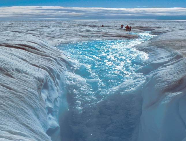

Figure 2. Record of atmospheric temperature, CO2 and CH4 extracted from Antarctic ice core by Petit et al. (Nature,
399, 429, 1999)

                                                        5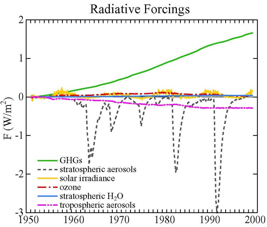

Figure 3. Climate was dramatically different than today during the last ice age, which peaked 20,000 years ago.
Global climate forcing was about 6½ W/m2 less than in the current inter-glacial period. This forcing maintained a
planet 5°C colder than today. [Drawing from Reports to the Nation, Fall, 1997.]

                                                          6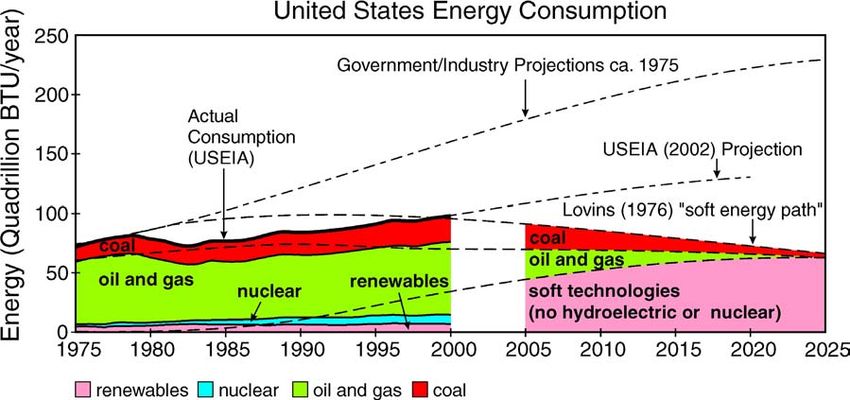

Box 2: But What About…

“Last winter was so cold! I don’t notice any global warming!” Global warming is ubiquitous,
but its magnitude so far is only about 1°F. Day-to-day weather fluctuations are of order 10°F.
Even averaged over a season this natural (year-to-year) variability is about 2°F, so global
warming does not make every season warmer than a few decades ago. However, global
warming already makes the probability of a warmer than “normal” season about 60%, rather than
the 30% that prevailed in 1950-1980 [Plate XV in Carl Sagan’s Universe, Cambridge Univ.
Press, 282 pp., 1997].

“I read that satellites measure global cooling, not warming.” That was the story a few years
ago, but as the satellite record has lengthened and been studied more carefully it has shifted to
warming. The discrepancy with surface measurements is disappearing. The primary issue now
is: “how fast is the warming?”

“The surface warming is mainly urban ‘heat island’ effects near weather stations.” Not so.
As predicted, the largest warming is found in remote regions such as central Asia and Alaska.
The largest areas of surface warming are over the ocean, far from urban locations [see maps at
http://www.giss.nasa.gov/data/update/gistemp]. Temperature profiles in the solid earth, at
hundreds of boreholes around the world, imply a warming of the continental surfaces between
0.5 and 1°C in the past century.

“The warming of the past century is just a natural ‘rebound’ from the ‘little ice age’.” Any
rebound from the European little ice age, which peaked in 1650-1750, would have been largely
complete by the 20th century. Indeed, the natural long-term climate trend is to a colder climate.

“Isn’t human-made global warming saving us from the next ice age?” Yes, but the gases that
we have added to the atmosphere are already far more than needed for that purpose.

“Climate variations are mainly due to solar variability.” The sun does flicker and the ‘little ice
age’ may have been caused, at least in part, by reduced solar output. Best estimates are that the
sun contributed about one quarter of global warming between 1850 and 2000. Climate forcing
by greenhouse gases is now larger than that by the sun, and the greenhouse forcing is increasing
monotonically while no significant long-term trend is expected for the sun. The sun may
contribute to future climate change, but it is no longer the dominant player.

“Global warming will be negligible if the “iris effect”, suggested by Richard Lindzen, is valid.”
This proposed negative climate feedback (in which it is supposed that tropical clouds adjust to
allow more heat radiation to escape to space when the Earth gets warmer) has been discredited in
specific tests against in situ and satellite data. More generally, any feedbacks that exist in the
real world are included in the empirical measures of climate sensitivity provided by the history
of the Earth. This history shows that the Earth's climate is sensitive to forcings, with a sensitivity
similar to that of climate models.

                                                  7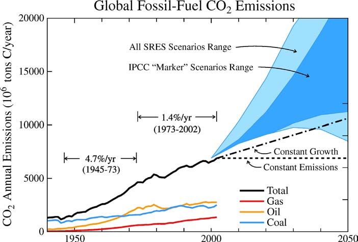

Climate Forcing Agents Today
The largest change of climate forcings in recent centuries is caused by human-made greenhouse
gases. These gases absorb the Earth’s infrared (heat) radiation. Because they make the
atmosphere more opaque in the infrared region, the Earth’s radiation to space emerges from a
higher level in the atmosphere where it is colder. The energy radiated to space is thus reduced,
causing a temporary planetary energy imbalance, with the Earth absorbing more energy from the
sun than it radiates to space. Thus the Earth gradually warms, but it requires about a century to
return most of the way to equilibrium, because of the large heat capacity of the oceans. In the
meantime, before it achieves equilibrium, more forcings may be added.
        The single most important human-made greenhouse gas is CO2, which comes mainly
from burning of fossil fuels (coal, oil and gas). However, the combined effect of the other
human-made gases is comparable to that of CO2. These other gases, especially tropospheric
ozone (O3) and its precursors including methane (CH4), are ingredients in atmospheric smog that
damages human health and agricultural productivity.
        Aerosols (fine particles in the air) are, besides greenhouse gases, the other main human-
made climate forcing. Aerosols cause a more complex climate forcing than that by greenhouse
gases. Some aerosols, such as sulfates arising from sulfur in fossil fuels, are highly reflective
(white) and thus reduce solar heating of the Earth. However, black carbon (soot), a product of
incomplete combustion of fossil fuels, biofuels and outdoor biomass burning, absorbs sunlight
and thus heats the atmosphere.
        This aerosol direct climate forcing is uncertain by at least 50%, in part because aerosol
amounts are not well measured. In addition, the black carbon effect is complex. In regions of
heavy soot, such as India and China, sunlight at the surface is reduced, causing a local surface
cooling. However, the heating of the air at higher levels results in surface warming on global
average, through its influence on atmospheric stability and cloud cover. These effects must be
computed with global climate models, and their magnitude differs from one model to another.
        Aerosols also cause an indirect climate forcing by altering the properties of cloud drops.
Human-made aerosols increase the number of condensation nuclei for cloud drops, thus causing
the average size of the cloud drops to be smaller. The larger number of smaller drops makes the
clouds slightly brighter. Smaller drops also make it more difficult for the clouds to produce rain,
thus increasing average cloud lifetime. Brighter long-lived clouds reduce the amount of sunlight
absorbed by the Earth, so the indirect effect of aerosols is a negative forcing that causes cooling.
        Other human-made climate forcings include replacement of forests by cropland. Forests
are dark even with snow on the ground, so their removal reduces solar heating.
        Natural forcings, such as volcanic eruptions and fluctuations of the sun’s brightness,
probably have little trend on a time scale of 1000 years. However, evidence of a small solar
brightening over the past 150 years implies a climate forcing of a few tenths of 1 W/m2.
        The net value of the forcings added since 1850 is 1.6 ±1.0 W/m2. Despite the large
uncertainties, there is evidence that this estimated net forcing is approximately correct. One
piece of evidence is the close agreement of observed global temperature during the past several
decades with climate models driven by these forcings. More fundamentally, the observed heat
gain by the world ocean in the past 50 years is consistent with the estimated net climate forcing,
as discussed below.

                                                 8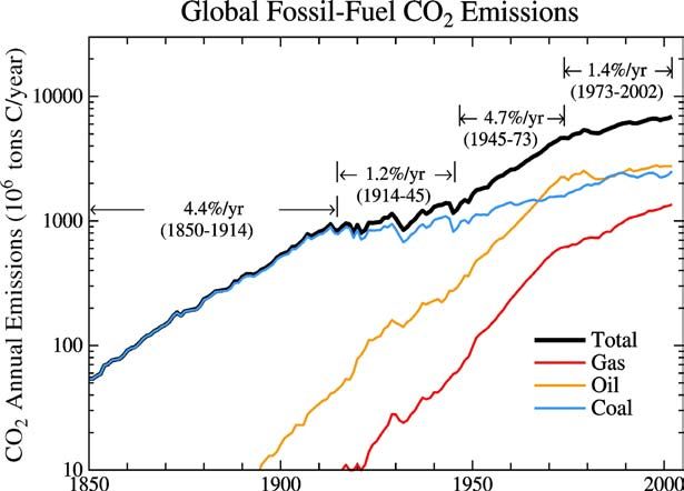

Figure 4. Climate forcing agents in the industrial era. Error bars are
                partly subjective 1σ (standard deviation) uncertainties.

•   Increases of well-mixed greenhouse gases (excludes O 3 ) are known accurately from in situ
    observations and bubbles of air trapped in ice sheets. For example, the increase of CO 2 from
    285 parts per million (ppm) in 1850 to 368 ppm in 2000 is accurate to about 5 ppm. The
    conversion of this gas change to a climate forcing (1.4 W /m 2 ), from calculation of the infrared
    opacity, adds about 10% to the uncertainty.
•   The CH 4 increase since 1850, including its effect on stratospheric H 2 O and tropospheric O 3 ,
    causes a climate forcing half as large as that by CO 2 . Principal anthropogenic sources of CH 4
    are landfills, coal mining, leaky natural gas lines, increasing ruminant population, rice
    cultivation, and anaerobic waste management lagoons. In the last decade the growth rate of
    CH 4 has slowed, suggesting that the growth of sources is slowing.
•   Tropospheric O 3 is increasing partly because CH 4 is increasing, but the primary cause is other
    human-made emissions, especially carbon monoxide, nitrogen oxides, and volatile organic
    compounds. Air quality regulations in the U.S. and Europe reduced O 3 precursor emissions in
    recent years, but not quite enough to balance increased emissions in the developing world.
•   Black carbon (“soot”), a product of incomplete combustion, can be seen in the exhaust of
    diesel-fueled trucks and buses. It is also produced by biofuels and outdoor biomass burning.
    Black carbon aerosols per se are not well measured, but their climate forcing is estimated from
    wide-spread multi-spectral measurements of total aerosol absorption. The estimated forcing
    includes the effect of soot in reducing the reflectance of snow and ice.
•   The reflective human-made aerosols are mainly sulfates, nitrates, organic carbon, and soil dust.
    Sources include fossil fuel burning and agricultural activities. Sources of the abundant sulfates
    are known reasonably well, but the 1σ uncertainty in the net forcing by reflective aerosols is at
    least 35%.
•   The indirect effects of aerosols on cloud properties are difficult to compute accurately, but
    recent satellite measurements of the correlation of aerosol and cloud properties are consistent
    with the estimated net forcing of –1 W /m2. The uncertainty is at least 50%.

                                                  9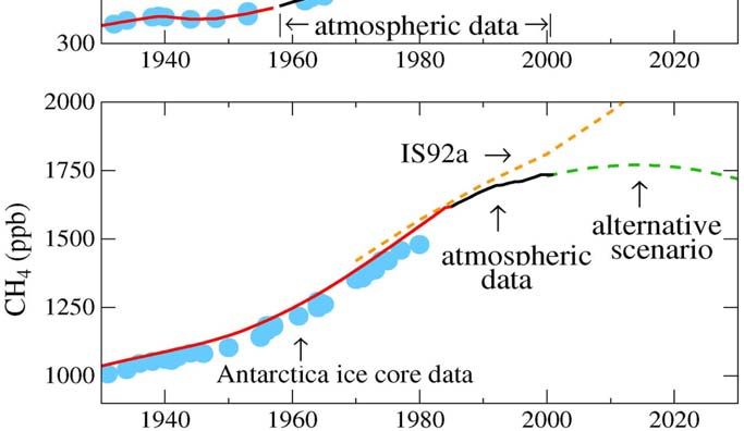

Global Warming
Global average surface temperature has increased about ¾°C (1.35°F) during the period of
extensive instrumental measurements, i.e., since the late 1800s. Most of the warming, about
½°C (0.9°F), occurred after 1950. The causes of observed warming can be investigated best for
the past 50 years, because most climate forcings were observed then, especially since satellite
measurements of the sun, stratospheric aerosols and ozone began in the 1970s. Furthermore,
70% of the anthropogenic increase of greenhouse gases occurred after 1950.
         Changes of known climate forcings since 1950 are shown in Figure 5. Largest forcings
are the positive forcing by greenhouse gases and negative forcing by aerosols. Stratospheric
aerosols, which are sulfates from occasional volcanic eruptions, are well-measured. However,
human-made aerosols, which have multiple sources and compositions, are poorly measured.
         These forcings have been used to drive climate simulations for 1951-1998 with the
NASA Goddard Institute for Space Studies SI2000 climate model [Reference 1b]. This model
has sensitivity ¾°C per W/m2, consistent with paleoclimate data and typical of other climate
models. The largest suspected flaws in the simulations are omission of poorly understood
aerosol effects on cloud drops and probable underestimate of black carbon changes. The first of
these is a negative forcing and the second is positive, so these flaws should be partially
compensating in their effect on global temperature.
         Simulated climate changes are compared with observations in Figure 6. The five model
runs differ only because of unforced (“chaotic” or “weather”) variability, which is an inherent
characteristic of complex coupled dynamical systems. The stratosphere in the model cools,
mainly due to ozone depletion, but it warms after volcanoes as the aerosols absorb thermal
radiation. The troposphere and surface warm due to increasing greenhouse gases, with brief
cooling intervals caused by large volcanoes. These changes are in accord with observations, as
illustrated. However, it would be a mistake to take this agreement as quantitative confirmation
of the principal model parameters and assumptions. A larger (smaller) value for the net climate
forcing could yield comparable agreement with the observations, if it were combined with a
smaller (larger) value of climate sensitivity. Also, unforced (chaotic) variability in this specific
version of the GISS model is probably less than unforced variability of real world climate.
         The most important quantity is the planetary energy imbalance (Figure 6d). This
imbalance is a consequence of the long time that it takes the ocean to warm. We conclude that
the Earth is now out of balance by something between 0.5 and 1 W/m2, i.e. there is that much
more solar radiation being absorbed by Earth than heat being emitted to space. One implication
of this imbalance is that, even if atmospheric composition does not change further, the Earth’s
surface will eventually warm another 0.4-0.7°C.
         The Earth’s energy imbalance is a vital statistic, because it is the residual climate forcing
that the planet has not yet responded to. It is too small to be measured directly, but we can verify
its value because the only place that the energy can be going is into melting ice or heating the air,
land and ocean. It is worth examining simple calculations of these energy sinks, because, as we
show in the next section, this provides insight about prospects for future global changes.
         As summarized in Box 4, most of the energy imbalance has been heat going into the
ocean. Sydney Levitus has analyzed ocean temperature changes of the past 50 years, finding that
the world ocean heat content increased about 10 W years/m2 in the past 50 years, consistent with
the time integral of the planetary energy imbalance. Levitus also finds that the rate of ocean heat
storage in recent years is consistent with our estimate that the Earth is now out of energy balance
by 0.5-1 W/m2. Note that the amount of heat required to melt enough ice to raise sea level one

                                                 10

Figure 5. Climate forcing in the past 50 years due to six mechanisms (GHGs = long-lived
            greenhouse gases). The tropospheric aerosol forcing is very uncertain [Reference 1b].

Box 4: Planetary Heat Storage: Ice, Air, Land and Ocean.
Estimates of the energy used to melt ice and warm the air, land and ocean in the past 50 years.1
Ice melting: assume that the 10 cm sea level rise between 1950 and 2000 was from melting ice (thermal
expansion of warming ocean water contributes about half the rise, but this error is partly balanced by melting sea
ice and ice shelves, which do not raise sea level). If the melted ice started at –10°C and ended at the mean ocean
surface temperature, +15°C, the energy used is 125 cal/g (100 cal/g for melting). The heat storage is thus
10g/cm2 × 125cal/g × 4.19 joules/cal × area Earth × 0.71 ~1.9 × 1022 joules ~ 1.2 watt-years.
Air warming: 0.5°C warming, atmospheric mass ~ 10 m of water, heat capacity air ~ 0.24 cal/g/°C, yields heat
storage in the air: 0.5°C × 1000 g/cm2 × 0.24 cal/g/°C × 4.19 joules/cal × area Earth ~ 0.26 ×1022 joules ~ 0.16
watt-years.
Land warming: The mean depth of penetration of a thermal wave into the Earth’s crust in 50 years, weighted by
∆T, is about 20 m. With a density ~ 3 g/cm3, heat capacity ~ 0.2 cal/g/°C, and 0.29 fractional land coverage of
Earth, the land heat storage is 2 ×103 cm ×3 g/cm3 × 0.2 cal/g/°C × 0.5°C ×4.19 joules/cal × area Earth × 0.29 ~
0.37 × 1022 joules ~ 0.23 watt-years.
Ocean warming: Levitus finds a mean ocean warming of 0.035°C in the upper 3 km of the ocean. The heat
storage is thus: 0.035°C × 3 × 105 g/cm2 × 1 cal/g × 4.19 joules/cal × area Earth × 0.71 ~ 16 × 1022 joules ~ 10
watt-years.
1
 Note that 1 watt-sec = 1 joule, # sec/year ~ π×107, area Earth ~ 5.1×1018 cm2, 1 watt-yr over full Earth ~
1.61×1022 joules, ocean fraction of Earth ~ 0.71, 1 calorie ~ 4.19 joules.

                                                        11

Figure 6. Simulated and observerd global temperature change for 1951-2000 and simulated
planetary energy imbalance [Reference 1b].

                                             12

meter is about 12 watt-years (averaged over the planet), energy that could be accumulated in 12
years if the planet is out of balance by 1 W/m2.
        The agreement with observations, for both the modeled temperature change and ocean
heat storage, leaves no doubt that observed global climate change is being driven by (natural and
anthropogenic) forcings. The current rate of ocean heat storage is a critical planetary metric,
because it determines the amount of additional global warming that is already “in the pipeline”.
It is important for a second, related, reason: it equals the reduction in climate forcings that we
would need to make if we wished to stabilize the Earth’s present climate.

The Time Bomb
The goal of the United Nations Framework Convention on Climate Change, produced in Rio de
Janeiro in 1992, is to stabilize atmospheric composition to “prevent dangerous anthropogenic
interference with the climate system” and achieve that in ways that do not disrupt the global
economy. The United States was the first developed country to sign the convention, which has
since been ratified by practically all countries. Defining the level of warming that constitutes
“dangerous anthropogenic interference” (DAI) is thus a crucial but difficult part of the global
warming problem.
        The United Nations established an Intergovernmental Panel on Climate Change (IPCC)
with responsibility for analysis of global warming. IPCC has defined climate forcing scenarios,
used these for simulations of 21st century climate, and estimated the impact of temperature and
precipitation changes on agriculture, natural ecosystems, wildlife and other matters [Reference
12a]. Significant effects are found, but even with warming of several degrees there are winners
and losers. IPCC estimates sea level change as large as several tens of centimeters in 100 years,
if global warming reaches several degrees Celsius. Their calculated sea level change is due
mainly to thermal expansion of ocean water, with little change in ice sheet volume.
        These moderate climate effects, even with rapidly increasing greenhouse gases, leave the
impression that we are not close to DAI. The IPCC analysis also abets the emphasis on
adaptation to climate change, as opposed to mitigation, in recent international discussions.
Adaptation is required, to be sure, because climate change is already underway. However, I will
argue that we are much closer to DAI than is generally realized, and thus the emphasis should be
on mitigation.
        The dominant issue in global warming, in my opinion, is sea level change and the
question of how fast ice sheets can disintegrate. A large portion of the world’s people live within
a few meters of sea level, with trillions of dollars of infrastructure. The need to preserve global
coast lines, I suggest, sets a low ceiling on the level of global warming that would constitute
DAI.
        The history of the Earth, and the present human-made planetary energy imbalance,
together paint a disturbing picture about prospects for sea level change. To appreciate this
situation we must consider how today’s global temperature compares with peak temperatures in
the current and previous interglacial periods, how long-term sea level change relates to global
temperature, and the time required for ice sheets to respond to climate change.
        Warmth in the Holocene peaked between 6000 and 10,000 years ago, but subsequent
cooling was slight. As shown by the Antarctic temperature record (Figure 2), the polar
temperature during the Holocene peak was about 1°C warmer than it was in the mid 20th century.
During the previous (Eemian) interglacial period polar temperatures were perhaps another 2°C
warmer. However, both paleoclimate data and climate models show that polar temperature

                                                13

change is about a factor of two larger than global mean temperature change. [The ice core
temperature anomalies at the pole refer to the inversion level, where the snow is formed; surface
air anomalies are slightly larger (Reference 2d).]
         This means that, with the 0.5°C global warming of the past few decades, the Earth’s
average temperature is just now passing through the peak Holocene temperature level.
Furthermore, the current planetary energy imbalance of about ¾ W/m2 implies that global
warming already “in the pipeline”, about another 0.5°C, will take us about halfway to the global
temperature that existed at the peak of the Eemian period.
         Sea level during the Eemian is estimated to have been 5-6 meters (16-20 feet) higher than
it is today. Although the geographical distribution of climate change influences the effect of
global warming on ice sheets, paleoclimate history suggests that global temperature is a good
predictor of eventual sea level change. The main issue is: how fast will ice sheets respond to
global warming?
         IPCC calculates only a slight change in the ice sheets in 100 years. However, the IPCC
calculations include only the gradual effects of changes in snowfall, sublimation and melting. In
the real world, ice sheet disintegration is driven by highly nonlinear processes and feedbacks.
The peak rate of deglaciation following the last ice age was a sustained rate of melting of more
than 14,000 km3/year, about one meter of sea level rise every 20 years, which was maintained for
several centuries. This period of most rapid melt, meltwater pulse 1A, coincided, as well as can
be measured, with the time of most rapid warming (Reference 2d).
         Given the present unusual global warming rate on an already warm planet, we can
anticipate that areas with summer melt and rain will expand over larger areas of Greenland
(Figure 7) and fringes of Antarctica. This will darken the ice surface in the season when the sun
is high, promote freeze-thaw ice breakup, and, via ice crevasses, provide lubrication for ice sheet
movement. Rising sea level itself tends to lift marine ice shelves that buttress land ice,
unhinging them from anchor points. As ice shelves break up, this accelerates movement of land
ice to the ocean.
         This qualitative picture of nonlinear processes and feedbacks is supported by the
asymmetric nature of glacial cycles (Figure 3) and the high rate of sea level rise associated with
rapid warming. Although building of glaciers is slow, once an ice sheet begins to collapse its
demise can be spectacularly rapid. The building of an ice sheet is a dry process, limited by the
annual snowfall rate, and thus requires millennia. Ice sheet disintegration, on the other hand, is a
wet process, nourished by positive feedbacks, and thus, once underway, it can proceed much
more rapidly.
         This natural melting process will be accelerated by the human-induced planetary energy
imbalance. This imbalance provides an ample supply of energy for melting ice (Box 4), which
can be delivered to the ice via ocean currents, atmospheric winds, and rainfall, as well as by
icebergs drifting to lower latitudes. Furthermore, this energy source is supplemented by
increased absorption of sunlight by ice sheets darkened by black carbon aerosols, as discussed
below, and the positive feedback process as melt-water darkens the ice surface.
         A planetary energy imbalance of +1 W/m2, maintained for a century, would cause a sea
level rise of about 8 meters, if the energy went entirely into melting of ice (Box 4). In the 20th
century most of the planetary energy imbalance went into warming of the ocean. In the future,
as the planet warms, an increasing fraction of the planetary energy imbalance is likely to go into
melting of ice, as significant portions of the ice sheets become wetter, softer, and more mobile.
The flux of energy that goes into melting will be increased by positive feedbacks. One feedback

                                                14

is caused by the increasing area of summer melt and lengthening melt season, as the wetter,
darker snow and ice surfaces absorb more sunlight. A second feedback is caused by the
tendency of melt-water to cool the polar sea surface, thus increasing the regional planetary
energy imbalance and the downward flux of energy. A third process affecting the rate of ice
melt is caused by increasing ocean surface temperatures at low and middle latitudes, which will
increase the transport of energy to the ice sheets. The prime mechanism for this is likely to be
the latent energy carried by occasional summer storms delivering heavy rainfall on portions of
the ice sheet, which could be very effective in speeding ice sheet motion and disintegration.
        Such multiple positive feedbacks ultimately can drive non-linear disintegration of large
portions of the ice sheets. This is a likely explanation for the rapid ice sheet collapse in melt-
water pulse 1A (about 5 meters of sea level rise per century). It can be argued that in this
paleoclimate case the ice sheets had a long period of preconditioning before the ice collapsed.
On the other hand, it should be noted that the forcing was small in the paleoclimate case and
changed only slowly over millennia. Now, on the contrary, there is a continual relentless forcing
caused by a large human-made planetary energy imbalance that provides ample energy to rapidly
erase the cooling effect of melting ice that tends to slow the paleoclimate response.
        These considerations do not mean that we should expect large sea level change in the
next few years. Preconditioning of ice sheets for accelerated break-up may require a long time,
perhaps many centuries. However, I suspect that a significant measurable increase in the rate of
sea level rise could begin within decades, especially if the planetary energy imbalance continues
to increase. Such a change would presage much larger sea level change over the next century or
two, because of several long time constants in the system: (1) several decades required for major
changes of energy systems and thus greenhouse gas emissions, (2) several decades to a century
for the climate system to approach equilibrium with changed climate forcings, (3) the time
required for ice sheets to respond in a substantial way to changed climate forcings and changed
climate, which I suggest may be as small as several centuries or less.
        Whatever the preconditioning period for ice sheet disintegration is, these long time
constants and the associated system inertia imply that global warming beyond some limit will
create a legacy of large sea level change for future generations. And once this process has
passed a certain point, it will be impractical to stop. The same inertia of the ice sheets, which
discourages rapid change, is a threat for the future. It will not be possible to build walls around
Greenland and Antarctica. Dykes may protect limited regions, such as Manhattan and the
Netherlands, but most of the global coastlines will be inundated.
        I argue that the level of DAI is likely to be set by the global temperature and planetary
radiation imbalance at which substantial deglaciation becomes practically impossible to avoid.
Based on the paleoclimate evidence discussed above, I suggest that the highest prudent level of
additional global warming is not more than about 1°C. In turn, given the existing planetary
energy imbalance, this means that additional climate forcing should not exceed about 1 W/m2.
        Detection of early signs of accelerating ice sheet breakup, and analysis of the processes
involved, may be provided by the satellite IceSat recently launched by NASA. IceSat will use
lidar and radar to precisely monitor ice sheet topography and dynamics. We may soon be able to
investigate whether or not the ice sheet time bomb is approaching detonation.

                                                15

Figure 7. Surface melt on the Greenland ice sheet descending into a moulin. The
moulin is a nearly vertical shaft, worn in the glacier by the surface water, that
carries the water to the base of the ice sheet. [Photo courtesy of Roger Braithwaite
and Jay Zwally.]

  Figure 8. Climate forcing scenario for 2000-2050 that yields a forcing of
  0.85 W/m2 (colored bars) [Reference 1a].

  Figure 9. Growth rate of climate forcing by well-mixed greenhouse gases (5-year
  mean), O3 and stratospheric H2O, which were not well measured, are not included
  [Reference 1a].

                                       16

Climate Forcing Scenarios
The IPCC defines many climate forcing scenarios for the 21st century based on multifarious
“story lines” for population growth, economic development, and energy sources. The scenarios
lead to a wide range for added climate forcings in the next 50 years (vertical bars in Figure 8).
         The IPCC added climate forcing in the next 50 years is 1-3 W/m2 for CO2 and 2-4 W/m2
with other gases and aerosols included. Even their minimum added forcing, 2 W/m2, would
cause DAI with the climate system, based on our criterion. Further, IPCC studies suggest that
the Kyoto Protocol, designed to reduce greenhouse gas emissions from developed countries,
would reduce global warming by only several percent. Gloom and doom seem unavoidable.
         However, are the IPCC scenarios necessary or even plausible? There are reasons to
believe that the IPCC scenarios are unduly pessimistic. First, they ignore changes in emissions,
some already underway, due to concerns about global warming. Second, they assume that true
air pollution will continue to get worse, with O3, CH4 and BC all greater in 2050 than in 2000.
Third, they give short shrift to technology advances that can reduce emissions in the next 50
years.
         An alternative way to define scenarios is to examine current trends of climate forcing
agents, to ask why they are changing as observed, and to try to understand whether there are
reasonable actions that could encourage further changes in the growth rates. Precise data are
available for trends of the long-lived greenhouse gases (GHGs) that are well-mixed in the
atmosphere, i.e., CO2, CH4, N2O and CFCs (chlorofluorocarbons).
         The growth rate of the GHG climate forcing peaked in the early 1980s at a rate of almost
0.5 W/m2 per decade, but declined by the 1990s to about 0.3 W/m2 per decade (Figure 9). The
primary reason for the decline was reduced emissions of CFCs, whose production was phased
out because of the destructive effect of CFCs on stratospheric ozone.
         The two most important GHGs, with CFCs on the decline, are CO2 and CH4. The growth
rate of CO2, after surging between the end of World War II and the mid-1970s, has since almost
flattened out to an average growth rate of 1.7 ppm/year over the past decade (Figure 10a).
Although the exponential growth rate of CO2 has slowed, the annual increments of atmospheric
CO2 continue to increase, and they are likely to continue to grow until annual CO2 emissions
flatten out or begin to decline. The annual CO2 increment has exceeded 2 ppm/year in three of
the past six years. The CH4 growth rate has declined dramatically in the past 20 years, by at least
two-thirds (Figure 10b).
         These growth rates are related to the rate of global fossil fuel use (Figure 11). Fossil fuel
emissions increased by more than 4%/year from the end of World War II until 1975, but
subsequently by just over 1%/year. The change in fossil fuel growth rate occurred after the oil
embargo and price increases of the 1970s, with subsequent emphasis on energy efficiency. CH4
growth has also been affected by other factors including changes in rice farming and increased
efforts to capture CH4 at landfills and in mining operations.
         If recent growth rates of these GHGs continued, the added climate forcing in the next 50
years would be about 1.5 W/m2. To this must be added the (positive or negative) change due to
other forcings such as O3 and aerosols. These forcings are not well-monitored globally, but it is
known that they are increasing in some countries while decreasing in others. Their net effect
should be small, but it could add as much as 0.5 W/m2. Thus, if there is no slowing of emission
rates, the human-made climate forcing could increase by 2 W/m2 in the next 50 years.
         This “current trends” growth rate of climate forcings, 2 W/m2 in 50 years, is at the low
end of the IPCC range of 2-4 W/m2. The IPCC 4 W/m2 scenario requires 4%/year exponential

                                                 17

growth of CO2 emissions maintained for 50 years and large growth of air pollution. The 4 W/m2
scenario yields dramatic climate change for the media to fixate upon, but it is implausible.
        Although the “current trends” scenario of 2 W/m2 in 50 years is at the low end of the
IPCC range, it is larger than the 1 W/m2 level that we suggested as our current best estimate for
the level of DAI. This raises the question of whether there is a feasible scenario with still lower
climate forcing.

A Brighter Future
I have discussed elsewhere [Reference 6] a specific “alternative scenario” that keeps added
climate forcing in the next 50 years at about 1 W/m2. Expected global warming by 2050 is
between ½°C and ¾°C, i.e., a warming of about 1°F [References 1b, 1c].
          This alternative scenario has two components: (1) halt or reverse growth of air pollutants,
specifically soot, O3, and CH4, (2) keep average fossil fuel CO2 emissions in the next 50 years
about the same as today. The CO2 and non-CO2 portions of the scenario are equally important. I
argue that they are both feasible and make sense for other reasons, in addition to climate.
          Air pollution. Is it realistic to stop the growth of air pollution, or even achieve some
reduction? A million people die every year from air pollution, with large economic cost.
Actions to improve air quality have been initiated already in the United States and Europe, and
still stricter standards are likely. In developing countries, such as India and China, air pollution
is already about as bad as can be tolerated. Discussions among scientists from developed and
developing countries [Reference 3] suggest that cleaner air is practical, and achievement could
be speeded if there were concerted efforts to develop and share cleaner technologies.
          Emphasis should be placed, in addressing air pollution, on the constituents that contribute
most to global warming. Methane, a precursor of O3, offers a great opportunity to halt the
growth of a substance that has been expected to contribute much to future global warming. If
human sources of CH4 are reduced, it may even be possible to get the atmospheric CH4 amount
to decline, thus providing a cooling that would partially offset the CO2 increase. Reductions of
black carbon (BC) aerosols would help counter the warming effect of reductions in sulfate
aerosols. O3 precursors, besides CH4, especially nitrogen oxides and volatile organic
compounds, must be reduced to decrease low-level O3, the prime component of smog, which
damages the human respiratory system and agricultural productivity.
          Actions needed to reduce CH4, such as methane capture at landfills, waste management
facilities, and fossil fuel mining, have economic benefits that partially offset the costs. Prime
sources of BC are diesel fuels and biofuels. These sources need to be dealt with for health
reasons. The tiny BC aerosols spewed out in the burning of these fuels are microscopic sponges
that soak up toxic organic carbon emitted in the same burning process. When these minuscule
soot particles are breathed into the lungs they penetrate human tissue deeply. Some enter the
bloodstream and are suspected of being the primary carcinogen in air pollution. Diesel could be
burned more cleanly with improved technologies. However, there may be even better solutions,
such as hydrogen fuel, which would eliminate ozone precursors as well as soot.

        Carbon dioxide. CO2 will be the dominant anthropogenic climate forcing in the future.
Is the CO2 portion of the alternative scenario feasible? It would require a near-term leveling off
of fossil fuel CO2 emissions and a decline of CO2 emissions before mid-century, heading toward
stabilization of atmospheric CO2 by the end of the century. Near-term leveling of emissions

                                                 18

Figure 10. Growth rates of atmospheric CO2 and CH4 [Reference 1a;
data update by Ed Dlugokencky and Tom Conway, NOAA Climate
Monitoring and Diagnostics Laboratory].

Figure 11. Global fossil fuel CO2 emissions based on data of Marland
and Boden [References 1a and 11]; 2001-2002 update based on
Reference 11b.

                             19

Figure 12. Projections of U.S. energy use made in the early 1970s compared with actual use. The growth
of “soft” energy technologies (renewable energies, excluding large hydroelectric dams) advocated by
Lovins has not occurred to a noticeable extent, but his projection of total energy use was quite accurate.

Figure 13. Observed CO2 and CH4 amounts, compared with the typical IPCC scenario and the
“alternative scenario”. The alternative scenario falls below all IPCC scenarios for both CH4 and CO2 (see
Appendix). In situ observations are available from the NOAA Climate Monitoring and Diagnostics
laboratory. CH4 in Antarctica is less than global mean CH4 because the CH4 sources are primarily in the
Northern Hemisphere [update of Reference 6a].

                                                   20

might be accomplished via improved energy efficiency and increased use of renewable energies,
but a long-term decline of emissions will require development of energy technologies that
produce little or no CO2 or that capture and sequester CO2.
         The plausibility of flattening near-term CO2 emissions is suggested by the history of
emissions (Figure 11). The reduction from 4% annual growth to just over 1% was accomplished
mainly via improved energy efficiency and without a concerted global scale effort. Current
technologies provide great potential for more efficiency improvements (Reference 5). The
growth rate of reported global fossil fuel CO2 emissions in the 1990s was about 1%/year, despite
robust economic growth in the United States, China, and the world as a whole (see Appendix).
Concerted efforts at efficiencies and renewable energies have the potential to squeeze out an
additional 1% in the near-term. The evidence indicates that this additional slowdown of
emissions will not occur with “business-as-usual” conditions, as recent CO2 emissions have
continued to grow at an average of 1 to 1.5% per year, but rather it will require a concerted effort
to reduce emissions.
         Long-term reduction of CO2 emissions is a greater challenge, as energy use will continue
to rise. Progress is needed across the board: continued efficiency improvements, more
renewable energy, and new technologies. Next generation nuclear power, if acceptable to the
public, could be an important contributor. There may be new technologies before 2050 that we
have not imagined. A fallback, should greater fossil fuel use be necessary, is capture and
sequestration of CO2.
         The impact of continual energy efficiency improvements must be recognized. Some
analysts project a quadrupling of world energy needs by 2050 to 50 Terawatts (power use today
is 10 Terawatts of fossil fuel energy and 2 Terawatts from other sources). These same persons
have been projecting such energy growth rates for years without comparing their prior
predictions with data.
         As an informative example, we compare in Figure 12 projections of United States energy
use made in the early 1970s with actual energy use. The data show that energy use increased
about 1% per year over the past three decades, far below most projections. Only in the past few
years has energy use crept above the level that Amory Lovins, an advocate of energy
efficiencies, had projected, and then only because the trend toward improving mileage of
passenger vehicles was reversed in the past decade. Note that a moderate 1% per year growth in
energy use was achieved in a period when the real cost of (fossil fuel) energy was declining. The
flat energy usage from the 1970s to the 1980s was aided by energy price increases in the 1970s.
         The growth of “soft” energy technologies (renewable energies, excluding large
hydroelectric dams) advocated by Lovins has not occurred to an extent sufficient to even show
up in Figure 12. On the other hand, Lovins’ projection of total energy use was accurate. Many
opportunities exist for continuing improvements of energy efficiency, e,g,. in solid state lighting
and in transportation. Thus it may be practical for total energy use in the U.S. to remain nearly
flat for a substantial period. Furthermore, U.S. CO2 emissions will increase less than energy use
if renewable energy contributions are increased. Thus it seems feasible for U.S. CO2 emissions
to be flat or even decline.
         Improvements of energy efficiency and moderation of energy growth rates are not limited
to the U.S. Indeed, the U.S. fractions of global energy use and CO2 emissions actually increased
slightly in the past decade (Reference 1a). Realistic moderate global energy growth rates,
coupled with near-term emphasis on renewable energies and long-term technology development,
could keep global CO2 emissions flat in the near-term and allow the possibility of long-term

                                                21

reductions, as may be required to avoid dangerous anthropogenic interference with climate.
Quantitative CO2 scenarios of this sort are presented in the Appendix.
         Observed trends. Observed global CO2 and CH4 are shown in Figure 13. It is apparent
that the real world is beginning to deviate from the prototypical IPCC scenario, IS92a. It
remains to be proven whether the smaller observed growth rates are a fluke, soon to return to
IPCC rates, or are a meaningful difference. The concatenation of the alternative scenario with
observations is not surprising, since that scenario was defined with observations in mind.
However, in the three years since the alternative scenario was defined observations have
continued on that path. Although I have shown that the IPCC scenarios are unrealistically
pessimistic, I am not suggesting that the alternative scenario can be achieved without concerted
efforts to reduce anthropogenic climate forcings.
         The alternative scenario falls below all scenarios in IPCC (2001), as illustrated in the
Appendix: Climate Forcing Scenarios. The same is true for the other major climate forcings that
cause warming: CH4, tropospheric O3, and BC aerosols. It is likely that all these forcings are less
than the IPCC pathways, but, unfortunately, except for CH4 and CO2, they are not being
measured with an accuracy sufficient to define their rates of change.
         Summary. The strategy for dealing with climate change must evolve as the level of
forcing that produces “DAI” is better defined and as climate forcings are better measured.
Monitoring of the ice sheets, together with realistic ice sheet modeling, will help determine how
close the ice sheets are to accelerating retreat. Precise monitoring of ocean heat content
change, averaged over several years, will yield the sum of all current forcings. Measurements of
individual climate forcing agents will help define the most effective ways to stop global warming.

My Opinion: Scientific Uncertainties
        The above assessment involves personal judgments, even though it is based on data and
published papers. I included estimates of prime uncertainties, e.g., for climate sensitivity and
climate forcings. However, there will surely be surprises as we obtain more information about
climate forcings, observe actual climate change, and improve global climate models. In this
section I discuss two areas of uncertainty that I believe deserve special attention.
        Dangerous anthropogenic interference (“DAI”). Establishing the level of global
warming that constitutes DAI deserves greater attention than it has received. I argue that DAI
will be determined by the level of warming that threatens eventual large-scale disintegration of
the ice sheets. That is probably a good assumption if, indeed, a global warming only of the order
of 1-2°C is enough to initiate eventual removal of large portions of the Greenland or Antarctic
ice sheets.
        Why choose 1°C (relative to present global mean temperature) as a first estimate of the
level of DAI? This is based in part on the assertion that global mean temperature at the peaks of
the current (Holocene) and previous (Eemian) interglacial periods were only 0.5 and 1.5°C
warmer, respectively, than the mid-twentieth century temperature, and the fact that the Earth has
already warmed 0.5°C in the past 50 years. In presenting that argument, I used records of polar
temperature and the assumption that polar temperature changes are amplified by at least a factor
of two over global mean changes. However, in addition, global climate models driven by early
Holocene and Eemian boundary conditions provide strong supporting evidence that global mean
temperatures were not warmer than these estimated levels.
        Michael Oppenheimer [Reference 2b] also has used ice sheet stability as a basis to infer
the level of DAI, concluding that 2°C was his best estimate. His larger value is primarily a result

                                                22

of differing estimates for the global temperature in previous warm periods. I agree that the total
uncertainties in the level of DAI, including those discussed below, encompass both the 1°C and
2°C estimates. Furthermore, other scientists will argue that the level of DAI could be even larger
than 2°C. Indeed, Wild et al. [Reference 2c], using one of the most sophisticated GCMs with 1°
resolution, calculate that the Greenland and Antarctic ice sheets will grow with doubled CO2,
leaving only a modest sea level rise due mainly to thermal expansion of ocean water. In my
opinion, the IPCC calculations, epitomized by the Wild et al. result, omit the most important
physics, especially the non-linear effects of meltwater and secondarily the effects of black
carbon. Clearly it is crucial to define DAI more accurately. For example, if there is now 0.5°C
global warming “in the pipeline” then DAI = 2°C would permit three times as much additional
anthropogenic climate forcing as would DAI = 1°C. The Wild et al. results predict an even
higher DAI level.
        The time required for ice sheets to respond to global warming, commonly assumed to be
thousands of years, is another, related, aspect of the uncertainty in estimating DAI. IPCC
presumes a negligible change of ice sheet dynamics in the 21st century. I doubt that assumption,
because increased ice sheet movement surely must be driven by surface melt and percolation to
the ice sheet base, rather than penetration of a thermal wave through the solid ice. Surface melt
and summer precipitation associated with human-induced warming and planetary energy
imbalance are likely to be unusual by paleoclimate standards, and even the paleoclimate record
reveals instances of rapid ice sheet disintegration. The BØlling warming about 14 thousand
years ago, for example, was accompanied almost simultaneously by sea level rise at a rate of 4-5
meters per century (Reference 2d).
        Still another uncertainty is the magnitude of actual sea level rise during the Eemian
period. This is uncertain because uneven motions of the Earth’s crust make it difficult to
determine mean sea level change from the data available for a small number of sites. If Eemian
sea level was not much higher than that in the Holocene it would call into question our estimate
for DAI. However, it would not eliminate concern about the possibility of large sea level rise
due to the unique climate forcings in the budding “Anthropocene” era.
        There are additional interesting issues that could alter the ice sheet response to human
forcings. As discussed below, surface melt may be abetted by a slight aerosol darkening of the
ice sheet surface, which becomes especially effective in the warm season. Another curiosity is
that Antarctica (except the Antarctic Peninsula) and Greenland may have been “protected” in
recent decades by amplification of the polar vortices, i.e., a strengthening of the zonal winds that
has limited the warming in Greenland and Antarctica. To the extent that these enhanced zonal
winds are driven by ozone depletion, this “protection” may decrease in coming decades as the
Earth’s ozone layer recovers.
        It is apparent that there is considerable uncertainly about the level of global warming that
will constitute DAI. This should be an area of focused research in coming years, especially since
precise monitoring of ice sheet behavior is now possible. The NASA IceSat mission, monitoring
ice sheet topography with centimeter scale precision, should be used to revitalize glaciological
studies and test ice sheet modeling capabilities.
        Carbonaceous aerosols. Climate modelers should be puzzled by the large negative
forcings that aerosol scientists estimate as the direct and indirect effects of human-made fine
particles in the air. If these forcings were included in full in global climate models, the models
would tend to have cooling at middle latitudes in the Northern Hemisphere where the aerosols
are most abundant, as has been stressed by Peter Stone and associates (Reference 7). In reality,

                                                23