Impact of Climate Variability and Climate Change on Rainfall Extremes in Western Sydney and Surrounding Areas: Component 4 - Dynamical Downscaling ...
←
→
Page content transcription
If your browser does not render page correctly, please read the page content below
4L

     Impact of Climate Variability and Climate Change on
     Rainfall Extremes in Western Sydney and Surrounding
     Areas: Component 4 - Dynamical Downscaling
     Deborah Abbs and Tony Rafter
     29 September 2009

     Report to the Sydney Metro Catchment Management Authority and Partners

                                 1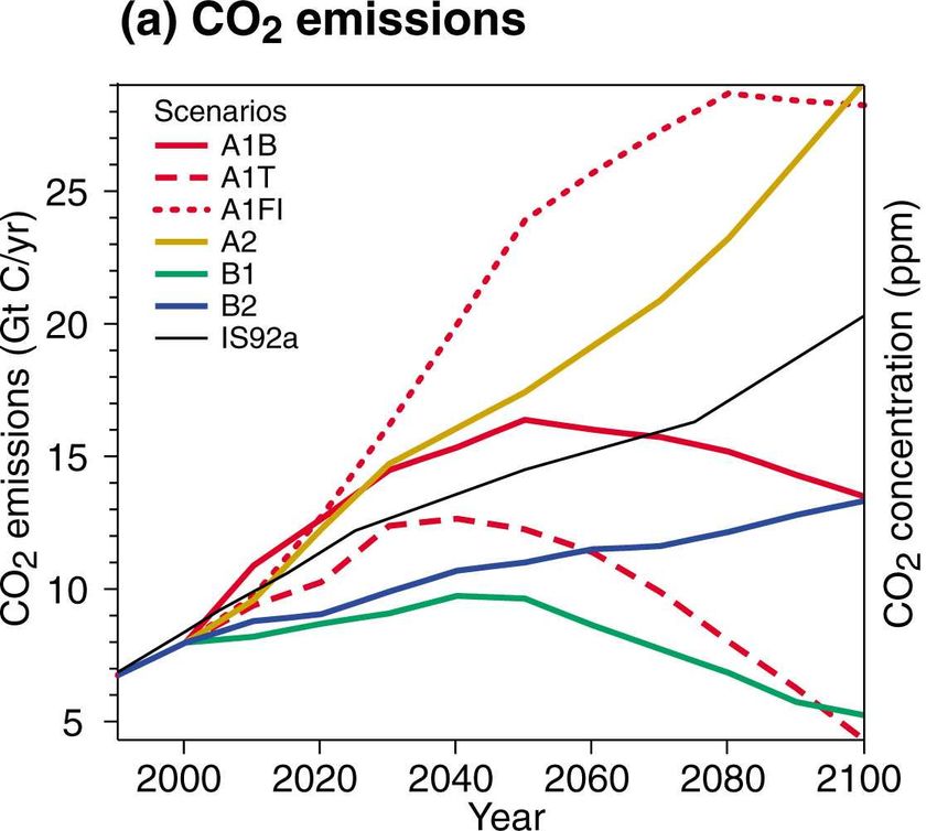
Enquiries should be addressed to:
Deborah Abbs
CSIRO Marine & Atmospheric Research
PMB No 1, Aspendale, Victoria, 3195
E-mail Deborah.Abbs@csiro.au

Distribution list
Chief of Division
Flagship Director
Project Manager
Client
Authors
Other CSIRO Staff
National Library
CMAR Libraries

Important Notice

    © Copyright Commonwealth Scientific and Industrial Research Organisation
    (‘CSIRO’) Australia 2008
    All rights are reserved and no part of this publication covered by copyright may be reproduced or
    copied in any form or by any means except with the written permission of CSIRO.
    The results and analyses contained in this Report are based on a number of technical, circumstantial
    or otherwise specified assumptions and parameters. The user must make its own assessment of the
    suitability for its use of the information or material contained in or generated from the Report. To the
    extent permitted by law, CSIRO excludes all liability to any party for expenses, losses, damages and
    costs arising directly or indirectly from using this Report.

Use of this Report

The use of this Report is subject to the terms on which it was prepared by CSIRO. In particular, the
Report may only be used for the following purposes.

•     this Report may be copied for distribution within the Client’s organisation;

•     the information in this Report may be used by the entity for which it was prepared (“the Client”), or by the
      Client’s contractors and agents, for the Client’s internal business operations (but not licensing to third
      parties);

•     extracts of the Report distributed for these purposes must clearly note that the extract is part of a larger
      Report prepared by CSIRO for the Client.

The Report must not be used as a means of endorsement without the prior written consent of CSIRO.
The name, trade mark or logo of CSIRO must not be used without the prior written consent of CSIRO.

                                                            2
Table of Contents
Executive Summary ................................................................................................... 7
1.      Introduction ..................................................................................................... 10
2.      Climate change................................................................................................ 12
        2.1     Impacts of climate change ...................................................................................... 12
        2.2     Uncertainties and climate change .......................................................................... 12
        2.3     Choice of scenario .................................................................................................. 15
3.      Data and models ............................................................................................. 17
        3.1     Study area & rainfall data ....................................................................................... 17
        3.2     NCEP Reanalysis data ........................................................................................... 18
        3.3     The Global and Regional Climate Models .............................................................. 18
4.      Climatology of extreme rainfall weather events............................................ 20
        4.1     Data, models and methodology .............................................................................. 20
        4.2     Synoptic typing ....................................................................................................... 20
                4.2.1         Synoptic classification of modelled extreme rainfall events ................................ 21
        4.3     Synoptic climatology of observed events ............................................................... 21
                4.3.1         Synoptic climatology of modelled events ............................................................ 27
                4.3.2         Impact of climate change .................................................................................... 28

5.      Dynamic downscaling of extreme rainfall ..................................................... 29
        5.1     Dynamical downscaling methodology .................................................................... 29
        5.2     Comparison with observed extreme rainfall and the impact of climate change. .... 30
                5.2.1         Spatial Patterns of Extreme Rainfall ................................................................... 31
                5.2.2         Extreme Value Analysis ...................................................................................... 33
        5.3     Impact of Climate Change ...................................................................................... 34
                5.3.1         Spatial Patterns of Climate Change .................................................................... 34
                5.3.2         Analysis of outputs for hydrological applications................................................. 44
        5.4     Recommendations for use in hydrological applications ......................................... 48
6.      Discussion & future work ............................................................................... 50
7.      References....................................................................................................... 52
APPENDIX A ............................................................................................................. 54
APPENDIX B ............................................................................................................. 69
APPENDIX C ............................................................................................................. 71
APPENDIX D ............................................................................................................. 74
APPENDIX E ............................................................................................................. 80

                                                                 iii
List of Figures

Figure 1: (a) Anthropogenic emissions and (b) atmospheric concentrations of carbon dioxide
    (CO2) for six SRES scenarios and the IS92a scenario from the IPCC Second
    Assessment Report in 1996 (IPCC 2001)....................................................................... 13
Figure 2: Projected change for 2046-2065 of the 20-year ARI 24-hour rainfall based on
    outputs from 9 international climate change GCMs forced with the A2 scenario. .......... 15
Figure 3: Location of Study Area........................................................................................... 17
Figure 4: The stretched grid of the cubic conformal atmospheric model. ............................. 19
Figure 5: (left) Composite MSLP fields for the synoptic types associated with extreme
    rainfall along the Central Coast of NSW. (right) Composite upper level fields for each
    type.................................................................................................................................. 23
Figure 6: Geographic distribution of (top) maximum rainfall associated with each of the 5
    synoptic types and (bottom) average rainfall associated with each type........................ 24
Figure 7: Seasonal occurrence of days with an MSLP pattern similar to those of extreme
    rainfall events.. ................................................................................................................ 25
Figure 8: Time series of the annual frequency of synoptics types based on the NCEP
    reanalyses. ...................................................................................................................... 26
Figure 9: High-resolution (4 km grid spacing) domain and terrain used for the simulations
    described herein.............................................................................................................. 30
Figure 10: Most extreme (a) 1-day rainfall and (b) 3-day rainfall for each grid point in the
    SILO dataset for the period 1960-1999. ........................................................................ 31
Figure 11: Simulated most extreme 2-hour rainfall for RAMS nested in (a) CC-Mk2, (b) CC-
    UK2 and (c) CC-M20....................................................................................................... 32
Figure 12: Simulated most extreme 24-hour rainfall for RAMS nested in (a) CC-Mk2, (b) CC-
    UK2 and (c) CC-M20....................................................................................................... 32
Figure 13: Simulated most extreme 72-hour rainfall for RAMS nested in (a) CC-Mk2, (b)
    CC-UK2 and (c) CC-M20. ............................................................................................... 32
Figure 14 : Spatial distribution of the 1980 100 year ARI 24-hour rainfall depth derived using
    outputs from RAMS nested in (a) CC-Mk2, (b) CC-UK2 and CC-M20. .......................... 34
Figure 15: Percentage change in rainfall depth for 2030 for 5 year ARI rainfall events for
    durations of 2, 24 and 72 hours ...................................................................................... 35
Figure 16: Percentage change in rainfall depth for 2030 for 100 year ARI rainfall events for
    durations of 2, 24 and 72 hours. ..................................................................................... 36
Figure 17: Percentage change in rainfall depth for 2070 for 5 year ARI rainfall events for
    durations of 2, 24 and 72 hours. ..................................................................................... 37
Figure 18: Percentage change in rainfall depth for 2070 for 100 year ARI rainfall events for
    durations of 2, 24 and 72 hours. ..................................................................................... 38
Figure 19: (a) 24-hour 100 year ARI rainfall depth from Australian Rainfall and Runoff (1987)
    and (b) ensemble average 1980 24-hour 100 year ARI rainfall depth based on the
    outputs from the 3 sets of RAMS simulations. ................................................................ 39
Figure 20: Ensemble average percentage change in rainfall depth for 2030 for (top) 5 year,
    and (middle) 100 year ARI rainfall events for durations of 2, 24 and 72 hours. ............. 41
Figure 21: Ensemble average percentage change in rainfall depth for 2070 for (top) 5 year,
    and (middle) 100 year ARI rainfall events for durations of 2, 24 and 72 hours. ............. 42
Figure 22: Ensemble average percentage change in rainfall depth for (top) 2030 and
    (middle) 2070 rainfall events for durations of 24 hours based on averaging the 10, 20 or
    50 most extreme events (vertical columns) from each set of simulations.. .................... 43

                                                                     iv
Figure 23: Sample return period curves for 24-hour and 72-hour rainfall accumulations for
    the locations indicated on the figures. ............................................................................ 45
Figure 24: Intensity-frequency-duration charts corresponding to 100 year ARI events for
    Penrith, Newcastle, Cordeaux, Cessnock, Katoomba and Parramatta. ......................... 47
Figure 25: Temporal curves for the study region for (a) 24-hour and (b) 72-hour rainfall
    bursts. ............................................................................................................................. 47
Figure 26: Locations of rainfall stations used to identify extreme rainfall days. Stations are
    colour-coded by post-1960 length of record. .................................................................. 68
Figure 27: (top) Observed accumulated rainfall and (bottom) modelled accumulated rainfall
    for the 7 cases studies identified..................................................................................... 73
Figure 28: As for Figure 20 but for a composite of R-CC-UK2 and R-CC-M20. ................... 74
Figure 29: As for Figure 21 but for a composite of R-CC-UK2 and R-CC-M20 .................... 75
Figure 30: As for Figure 20 but for a composite of R-CC-MK2 and R-CC-M20.................... 76
Figure 31: As for Figure 21 but for a composite of R-CC-MK2 and R-CC-M20.................... 77
Figure 32: As for Figure 20 but for a composite of R-CC-MK2 and R-CC-UK2.................... 78
Figure 33: As for Figure 21 but for a composite of R-CC-MK2 and R-CC-UK2.................... 79
Figure 34: As for Figure 22 but for 2-hour extreme rainfall events. ...................................... 80
Figure 35: As for Figure 22 but for 72-hour extreme rainfall events. .................................... 81

                                                                     v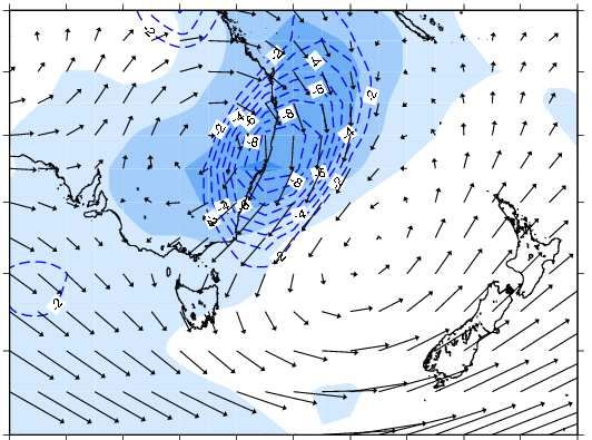
List of Tables

Table 1: The distribution of synoptic types for extreme rainfall events affecting the Central
    Coastal region of New South Wales ............................................................................... 22
Table 2: The occurrence of days with an MSLP pattern similar to those of extreme rainfall
    events.............................................................................................................................. 25
Table 3: The occurrence of days in the 3 climate models with an MSLP pattern similar to
    those of observed extreme rainfall events. av = annual average, s.d = standard
    deviation of yearly counts, total = total number of days per 40-year time slice, and % =
    percentage frequency of extreme rainfall type................................................................ 27
Table 4: Seasonal distribution of days in the 3 climate models with an MSLP pattern similar
    to those of observed extreme rainfall events. ................................................................. 28
Table 5: The total number of days per 40-year times slice in the 3 climate models with an
    MSLP pattern similar to those of observed extreme rainfall events. Results are
    presented for the 1980, 2030 and 2070 time slices........................................................ 28
Table 6: Projected percentage changes relative to 1980 in the intensity of 100 year ARI
    extreme rainfall events for durations of 2. 24 and 72 hours for Parramatta, Katoomba,
    Cordeaux, and Cessnock. Projected decreases are in red. .......................................... 49

                                                                    vi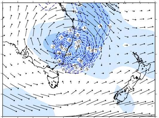
EXECUTIVE SUMMARY
In 2004, the Upper Parramatta River Catchment Trust expressed interest in undertaking a research
project on extreme rainfall events and it is the results from that study that are presented herein.

Floods are responsible for annual damages averaging $314 million, which is about 30% of all
Australian weather-related damages (BTE, 2001). Information about extreme rainfall intensity and
frequency for event-durations ranging from hours to multiple days is commonly needed for use in
flood impact, design and mitigation applications. Flood impact models also rely upon information
about how rapidly the average rainfall intensity increases with decreasing area, i.e. depth-area
curves. These relationships are likely to be altered by climate change. Quantifying these changes
requires very fine spatial resolution (4 km) and temporal resolution (hourly) using both dynamical
modelling and statistical methods. It is computationally intensive to quantify these changes
Australia-wide; thus, studies such as this are usually restricted to a relatively large area centred on
the region (or catchment) of interest.

Since the early 1970s scientists and policymakers have been aware of the possibility of human
activities impacting on the composition of the global atmosphere. By the mid 1980s atmospheric
observations had confirmed that the atmosphere was changing and over the following two decades
there has been a major international research effort to establish the nature of the changes and the
causes. Since the late 1980s the scientific findings on atmospheric change and the potential for
human based changes in the Earth’s climate have been reviewed and summarised by the
Intergovernmental Panel on Climate Change (IPCC).

Climate changes projections are based upon the outputs from global and regional climate models
that account for possible changes in the emissions of key greenhouse gases and aerosols. Studies
based on different climate models and emissions scenarios show that by 2100, differences in
emissions scenarios and different climate model sensitivities contribute similar amounts to the
uncertainty in global average surface temperature change. Projections of future regional climate
are subject to three key uncertainties. The first of these is related to uncertainties in greenhouse
gas emissions and the second is related to the climate sensitivity of climate models. Climate
sensitivity is a measure of the strength and rapidity of the surface temperature response to
greenhouse gas forcing. The third uncertainty is related to differing spatial patterns of change (i.e.
response of regional climate) between climate models. The development of climate change
projections on a regional scale relies upon analysing as many Global Climate Models (GCMs) and
Regional Climate Models (RCMs) as is feasible to ensure that uncertainty due to the climate
sensitivity of different models is captured. It is necessary to use model output available with a
daily temporal resolution to identify severe weather events, such as extreme rainfall and wind
events. However, daily model variables are not available for many of the GCM simulations to
which there is general access. Thus, our analysis is limited to the results from CSIRO climate
models. When considering results from a single (or small number of) model simulation(s), there is
concern as to the reliability and generality of the results and this concern needs to be considered
when using the results described herein.

Of the six illustrative scenarios chosen by the IPCC, the A2 scenario has been used for most global
climate modelling undertaken by CSIRO since the late 1990s and is the scenario considered in this
report. At that time, this scenario (one of self reliance, continuously increasing population,
regionally oriented economic growth and slow technological change) was considered to be a
“worst case” condition and thus considered to provide the upper bound for climate change

                                                   7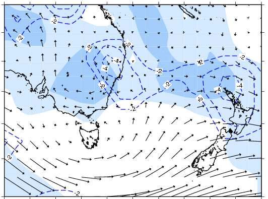
projections and the impacts of climate change. The IPCC recognised that the capacity of the
oceans and the terrestrial biosphere to absorb increasing emissions would decrease over time but
recent observations (e.g Rahmstorf et al., 2007; Canadell et al., 2007) suggest that absorptive
capacity has been falling more rapidly than estimated by the main models. If these trends continue,
a greater proportion of emitted carbon dioxide will remain in the atmosphere in the coming years
and this will exacerbate the warming trend consequences of these unexpectedly high levels of
emissions in the early years of the twenty-first century will be felt in future decades. Thus, it
appears that the choice of the A2 scenario can no longer be considered a “worst case” scenario and
now may be considered as “realistic” or even “optimistic”.

This study uses an “integrated hierarchy of models” as recommended in the IPCC Third
Assessment report (IPCC, 2001). In this approach, coarse resolution global and regional climate
models provide the initial and boundary conditions for progressively finer resolution models. In
general, these high-resolution simulations have been able to represent the spatial distribution of
extreme rainfall realistically and the magnitude of the extremes is close to observed, although there
is an apparent over-estimation of extremes in various mountainous regions.

Climate changes simulations based on climates representative of 2030 and 2070, show that there is
considerable spatial variation in the regions of extreme rainfall increase and the magnitude of that
increase. To overcome difficulties inherent in the analysis of spatially varying outputs, ensemble
averages and “consensus” maps were calculated.

Widespread increases in extreme rainfall intensity are not projected to occur until the second half
of the 21st Century and will predominantly be experienced by shorter duration events. By 2070 the
2-hour and 24-hour rainfall events are projected to experience widespread increases in intensity for
most regions. The 2-hours events are projected to experience a larger increase in intensity than the
24-hour and 72-hour events. By comparing the results obtained by averaging over the top 10 and
top 50 events it is apparent that the less frequent events are projected to experience greater
percentage increases in intensity than the more frequent events. In some locations, for example
west of Katoomba, the recurrence interval curves for the current climate and 2070 are likely to
cross, especially for rainfall durations of 24-hours and longer. For these durations the low
frequency events are projected to become more intense in the future and the higher frequency
events less intense. Thus, when extreme rainfall events occur in the future they are likely to be
characterised by more intense bursts of rainfall than currently occurs but, in many locations, with a
total accumulation smaller than occurs in the current climate. A comparison of the projections for
2030 indicates that the impact of global warming on extreme rainfall may be non-linear, with
widespread decreases in extreme rainfall intensity in the early 21st Century which gradually change
with time to become increases in extreme rainfall intensity.

Outputs from the Extreme Value Analysis (EVA) have been used to create (1) return period
curves, (2) intensity-frequency-duration curves for selected locations in the study region, and
temporal curves for the entire region. Examination of the return period and intensity-frequency-
duration curves, combined with the spatial patterns of change results, highlights the difficulty of
defining location-specific values for projected changes in extreme rainfall intensity due to climate
change. Recommendations to accounting for climate change in hydrological applications are
described and brief examples given. The temporal curves also suggest that in the future the main
rainfall burst in longer duration (i.e. 72-hour) events may occur earlier than at present.

The results form this study highlight the importance of considering the results from more than one
model when developing projections of climate change. The CCAM output used to initialise

                                                  8
RAMS in this study originates from simulations that have been undertaken between 2003 and
2007 using different versions and configuration of the model and different grid spacings. Ideally,
any future downscaling work should use a standard configuration and version of the model so that
this form of model uncertainty can be ruled out.
91. INTRODUCTION
The CSIRO Climatic Extremes research group (CER) is investigating rainfall intensity-frequency-
duration (IFD) and depth-area curves for western Sydney and surrounding areas for present day
and projected future conditions in collaboration with the Upper Parramatta River Catchment Trust
(now the Sydney Catchment Management Authority) and its partners. The other objectives of the
project are:
• Obtain a “broad brush” understanding of the likely changes in average and extreme
rainfall under enhanced greenhouse conditions (core).
• Quantify the likely future changes to the rainfall frequency characteristics of the study area
due to global warming (core).
• Assess the impact of decadal-scale climate fluctuations on rainfall frequency
characteristics (subsidiary).
The work plan consisted of four components couched within a three-year timeframe. The
objectives of Components 1 to 3 are to provide information on rainfall IFD and depth-area curves
for durations less than 6 hr for present day and projected future conditions, respectively. This
information is critical for flood design applications. The results from these components of the
project will be presented in a separate report.
This report presents the results from Component 4 of the project, specifically the high resolution
dynamical downscaling of extreme rainfall events for the current climate and the climates of 2030
and 2070. This component has been undertaken as a joint project with the Department of Climate
Change (formerly the AGO). The tasks are:
1. Identification of candidate cases,
2. High-resolution simulation of extreme rainfall events at a grid spacing of approximately
5km,
3. Analysis of downscaled events and preparation of IFD and depth-area curves for durations
of less than 1 hour to 72 hours.
Within this report results for three 40-year time slices are presented. The “1980” or current climate
refers to the climate for the atmosphere with greenhouse gas concentrations corresponding to the
1961-2000 period, while the “2030” climate has projected concentrations corresponding to the
2011-2050 period for the A2 scenario. Similarly the “2070” represents the 40 year timeslice 2051-
2090.
The report is set out as follows: Section 2 presents background information on climate change, it
describes the uncertainties inherent in the science and provide some background on scenarios and
the choice of scenario used in this report. Section 3 describes the data used in the dynamical
downscaling components of the project. It introduces the Global and Regional Climate Models
(GCMs and RCMs) and describes the observational data and climate model simulations utilised in
this study.
10In Section 4 we describe the synoptic typing procedure used to evaluate the skill of the regional
climate models in representing the synoptic situations associated with observed present-day
extreme precipitation events affecting the study region. Results and discussion from the synoptic
typing are presented here and the impact of climate change on these weather systems addressed.
The results from the dynamical downscaling are presented jn Section 5. These results are
presented in terms of maps showing the geographical distribution of the changes and graphs
illustrating changes to Average Recurrence Interval (ARI) and Intensity-Frequency-Duration
curves for selected locations. A discussion of the results is provided and recommendations as to
how best to use the results is provided.
112. CLIMATE CHANGE
2.1 Impacts of climate change
Since the early 1970s scientists and policymakers have been aware of the possibility of human
activities impacting on the composition of the global atmosphere. By the mid 1980s atmospheric
observations had confirmed that the atmosphere was changing and over the following two decades
there has been a major international research effort to establish the nature of the changes and the
causes. Since the late 1980s the scientific findings on atmospheric change and the potential for
human based changes in the Earth’s climate have been reviewed and summarised by the
Intergovernmental Panel on Climate Change (IPCC). The most recent report, the Fourth
Assessment Report on the Physical Science Basis of climate change (IPCC 2007) had the
following amongst its key conclusions:
• 'Global atmospheric concentrations of carbon dioxide, methane and nitrous oxide have
increased markedly as a result of human activities since 1750 and now far exceed pre-
industrial values determined from ice cores spanning many thousands of years '
• 'Warming of the climate system is unequivocal,'
• ‘Most of the observed increase in globally averaged temperatures since the mid-20th
century is very likely due to the observed increase in anthropogenic greenhouse gas
concentrations. …Discernible human influences now extend to other aspects of climate,
including ocean warming, continental average temperatures, temperature extremes and
wind patterns '
• 'Continued greenhouse gas emissions at or above current rates would cause further
warming and induce many changes in the global climate system during the 21st century
that would very likely be larger than those observed during the 20th century. '
2.2 Uncertainties and climate change
Climate changes projections are based upon the outputs from global and regional climate models
that account for possible changes in the emissions of key greenhouse gases and aerosols. The
emissions are those due to human activities, such as energy generation, transport, agriculture, land
clearing, industrial processes and waste. To provide a basis for estimating future climate change,
the IPCC began the development of a new set of greenhouse gas emissions scenarios in 1996
(IPCC, 2000) that attempt to account for future population growth, technological change and
social and political behaviour. The Special Report on Emissions Scenarios (SRES) produced a set
of 40 scenarios based around 4 different “storylines” that describe the relationships between the
forces driving the greenhouse gas emissions and their evolution (see Figure 1a). Carbon cycle
models are used to convert these emissions into atmospheric concentrations (Figure 1b), allowing
for various processes involving the land, ocean and atmosphere. Increasing concentrations of
greenhouse gases affect the radiative balance of the Earth. This balance determines the Earth’s
average temperature. These SRES greenhouse gas concentrations are converted to a radiative
forcing of the climate system.
12Figure 1: (a) Anthropogenic emissions and (b) atmospheric concentrations of carbon dioxide (CO2) for six
SRES scenarios and the IS92a scenario from the IPCC Second Assessment Report in 1996 (IPCC 2001).
Climate model equations are based on well-established laws of physics, such as conservation of
mass, energy and momentum and have been tested against observations. This provides a major
source of confidence in the use of models for climate projection. The other basis for confidence
comes from the ability of models to represent current and past climates, as well as observed
climate changes. The most important limitation of models is that a number of important physical
processes occur at scales too small to be explicitly resolved by the model, and therefore these have
to be represented in approximate form as they interact with the larger scales. Differences in the
representation of such processes are the principal cause of differences in the magnitude and
patterns of climate change found in different models. Climate model responses are most uncertain
in how they represent feedback effects, particularly those dealing with changes to cloud regimes
and ocean-atmosphere interactions. Studies based on different climate models and emissions
scenarios show that by 2100, differences in emissions scenarios and different climate model
sensitivities contribute similar amounts to the uncertainty in global average surface temperature
change.
Projections of future regional climate are subject to three key uncertainties. The first of these is
related to uncertainties in greenhouse gas emissions and the second is related to the climate
sensitivity of climate models. Climate sensitivity is a measure of the strength and rapidity of the
surface temperature response to greenhouse gas forcing. The third uncertainty is related to
differing spatial patterns of change (i.e. response of regional climate) between climate models.
The development of climate change projections on a regional scale relies upon analysing as many
Global Climate Models (GCMs) and Regional Climate Models (RCMs) as is feasible to ensure
that uncertainty due to the climate sensitivity of different models is captured. It is necessary to use
model output available with a daily temporal resolution to identify severe weather events, such as
extreme rainfall and wind events. However, daily model variables are not available for many of
the GCM simulations to which there is general access. Thus, our analysis is limited to the results
from CSIRO climate models. When considering results from a single (or small number of) model
simulation(s), there is concern as to the reliability and generality of the results and this concern
needs to be considered when using the results described herein.
13It is well known that there for any given application there is no one GCM that is superior to its
counterparts in every aspect of interest. Nevertheless, previous studies suggest that a handful of
models can be identified according to several (though incomplete) criteria. Suppiah et al. (2007)
used measures of RMS error and pattern correlations to evaluate 23 climate model simulations
performed for the IPCC 4th Assessment Report to produce climate change projections of
Australian rainfall and temperature. They found that the CSIRO Mark 3 GCM (the parent model
used in 2 of the 3 RCM simulations used herein) had a ranking of equal 11th out of the 23 models.
A second study (Perkins et al., 2007) used probability density functions of daily simulations of
precipitation, minimum temperature, and maximum temperature for 12 regions of Australia to
evaluate and rank coupled climate models used in the 4th Assessment Report of the IPCC. They
found that over all three variables considered the CSIRO Mark 3 GCM ranked second in skill.
Thus, in terms of Australian climate, the CSIRO Mark 3 GCM could be described as a “mid- to
upper-level performer”.
Rainfall changes are not directly forced by rising greenhouse gases but a warmer atmosphere can
hold more water vapour, and hence produce heavier rainfall. Rainfall over some parts of Australia
may change little, but elsewhere either decreases or increases may occur due to small differences
in the circulation and other processes, discussed above. Projected rainfall changes for Australia are
documented in CSIRO and Bureau of Meteorology, 2007. Near term projections (2030) are based
on the mid-range A1B scenario as model to model differences are larger than the differences
between the various emissions scenarios. “Over the next few decades, the variation in emissions
of greenhouse gases and aerosols represented by the SRES scenarios makes only a small
contribution to uncertainty in global warming (and by extension regional warming and other
changes in climate). This is because near-term changes in climate are strongly affected by inertia
in the climate system due to past greenhouse gas emissions, whereas climate changes later in the
century are more dependent on the particular pattern of greenhouse gas emissions that occur
through the century.” Projected changes for 2030, can be summarised as a decrease in annual
average rainfall for most of the continent, especially along the southern fringe. The ‘top end’ is
likely to experience little change in annual average rainfall. For projected changes centred on
2050 and 2070, variations are due to differences between both models and emission scenarios.
Projected changes for 2050 and 2070 for each of the emission scenarios are presents in Appendix
A of that report.
Extreme values statistics have been applied to the outputs from a suite of international climate
change simulations to create projections of changes in extreme rainfall intensity. The model
simulations used are relatively coarse-resolution global climate models that were completed and
made available for analysis as part of the IPCC’s Fourth Assessment Report published in 2007.
One of the simulations used in the extreme value analysis (CSIRO Mk3.0) has been further
downscaled and the results are presented in this report. Figure 2 shows projected changes, relative
to 1980, in the 20-year ARI for 2046-2065 for 9 of the models for the A2 scenario. These results
illustrate the uncertainty in climate change studies described above, in particular differing spatial
patterns of change (i.e. response of regional climate) between climate models.
14CSIRO MK3.0 GFDL CM2.0 CNRM CM3
CSIRO MK3.5 GFDL CM2.1 MRI CGCM
MIUB ECHO-G MPI ECHAM5 MIROC 3.2 (medres)
Figure 2: Projected change for 2046-2065 of the 20-year ARI 24-hour rainfall based on outputs from 9
international climate change GCMs forced with the A2 scenario.
The coarse spatial resolution of climate models remains a limitation on their ability to simulate the
details of regional climate change, especially changes in extreme events. Statistical and dynamical
downscaling techniques are used to translate the projections obtained from coarse-resolution
climate models to the catchment and rain-gauge scale required by hydrologists and planners.
Global and regional climate models show a broad qualitative agreement with the downscaled
results. However, downscaling is able to identify important localised regions of projected increases
in rainfall intensity not captured by the coarser models because the high resolution models are
better able to represent local topographic effects (orography and land-sea contrasts) and better able
to represent the convection that is a characteristic of extreme rainfall events.
2.3 Choice of scenario
The reader is referred to the report “Climate Change in Australia” (CSIRO and Bureau of
Meteorology, 2007) for a description of the four storylines that form the basis of the scenarios
used within climate change science. Of the six illustrative scenarios chosen by the IPCC, the A2
scenario has been used for most global climate modelling undertaken by CSIRO since the late
1990s and is the scenario considered in this report. At that time, this scenario (one of self reliance,
continuously increasing population, regionally oriented economic growth and slow technological
change) was considered to be a “worst case” condition and thus considered to provide the upper
bound for climate change projections and the impacts of climate change.
Rahmstorf et al (2007) present recent observed climate trends for carbon dioxide concentration,
global mean air temperature, and global sea level, and compare these trends to previous model
15projections as summarized in IPCC (2001). Their results suggest that the climate system may be
responding more quickly than climate models indicate. Their key results are:
• Since 1990 global mean surface temperature increase has been measured at 0.33ºC which
is in the upper end of the range predicted by the IPCC in the Third Assessment Report in
2001.
• Since 1990 the observed sea level has been rising faster than the rise projected by models,
as shown both by a reconstruction using primarily tide gauge data and, since 1993, by
satellite altimeter data. Sea level rise since 1993 has shown a linear trend of 3.3 ± 0.4
mm/year. In 2001, the IPCC projected a best estimate rise of less than 2mm/year.
They state “Overall, these observational data underscore the concerns about global climate
change. Previous projections, as summarized by IPCC, have not exaggerated but may in some
respects even have underestimated the change, in particular for sea level.”
The changes that have been observed to date are a result of historic emissions due to the lag in the
climate system resulting from the slow response of the oceans to absorb emissions. The IPCC
Fourth Assessment Report recognised that the capacity of the oceans and the terrestrial biosphere
to absorb increasing emissions would decrease over time. Observations suggest that absorptive
capacity has been falling more rapidly than estimated by the main models. If these trends continue,
a greater proportion of emitted carbon dioxide will remain in the atmosphere in the coming years
and this will exacerbate the warming trend (Canadell et al., 2007).
Global emissions of carbon dioxide have accelerated sharply since about 2000 due to increases in
fossil fuel burning and industrial processes, with this growth dominated by economic growth in
major developing countries such as China and India. Initial analysis carried out for the Garnaut
Review (Garnaut 2008) suggests the likelihood, under business as usual, of continued growth of
emissions in excess of the highest IPCC scenarios. Assuming more realistic growth and energy
intensity for China and India alone produces higher projected global emissions from fuel
combustion than even the most pessimistic of the IPCC scenarios out to 2030 (Sheehan and Sun,
2007). The consequences of these unexpectedly high levels of emissions in the early years of the
twenty-first century will be felt in future decades.
Thus, it appears that the choice of the A2 scenario can no longer be considered a “worst case”
scenario and now may be considered as “realistic” or even “optimistic”.
163. DATA AND MODELS
3.1 Study area & rainfall data
The study area has a homogeneous climate roughly bounded by longitudes 149.5º to 153º E; and
latitudes 31.5º to 36ºS. The focus is on the coastal drainage areas of this region only (i.e., the SW
corner of the region defined above would be ignored completely). The river basins included in the
study area are shown in Figure 3.
Figure 3: Location of Study Area
Rainfall data used in this component of the project comes from the Bureau of Meteorology’s
(BOM) rainfall network. This network includes over 6000 stations nation-wide, all of which
record daily rainfall using standardised equipment and observing protocols. The observations are
made at 0900 hours each day, with the 24-hour rainfall total being recorded against the day of
observation. Mostly these gauges are operated by volunteers, often at workplaces like post offices,
local government offices and farms. As a consequence, the quality of the data is quite variable,
even for different time periods at a single station. Details of the stations used are tabulated in
Appendix A.
Some of the data quality issues have been discussed by Lavery et al. (1992) and Viney and Bates
(2004). The data quality is affected by a number of reasons including observer’s inconsistencies
and exposure changes (changes in the height or structure of the gauge; changes in the windfield
associated with growing trees or the construction of nearby buildings).
Missing observations in the rainfall records arise from two main sources. The first appears to
relate to communication and data management issues. The second source of missing data occurs
when observers are absent from the station or otherwise unable to observe the gauge for a period
of one or more days. When the observer returns to the gauge it contains rainwater that potentially
17fell over a period of two or more days. In these circumstances the observer records the
accumulation period as well as the rainfall amount, which is entered against the date of
observation. Viney and Bates (2004) have discussed the issues related to these “untagged
accumulations”.
A second set of rainfall data have been used. These are gridded rainfall data obtained from the
SILO dataset (Jeffrey et al., 2001) produced and distributed by the Queensland Department of
Natural Resources, Mines and Energy. These data are interpolations derived from the Bureau of
Meteorology’s rainfall network. The quality of the data varies across Australia, depending on the
proximity of reporting stations. All plots based on observations use these data.
3.2 NCEP Reanalysis data
Mean sea level pressure (MSLP) data from the National Centers for Environmental Prediction
(NCEP) reanalysis dataset have been used to characterise the synoptic scale weather systems that
are conducive to extreme rainfall in the study region. The MSLP data are available in a gridded
format at a horizontal resolution of 2.5°× 2.5° (approximately 250 km) every six hours from 1958
to the present. In this study the MSLP data have been analysed twice daily for the extreme rainfall
events. Specific humidity, vertical velocity and winds at 850, 700 and 500 hPa have also been
analysed for the extreme rainfall days. These fields help identify the mechanisms that produce
extreme rainfall in the region.
3.3 The Global and Regional Climate Models
This study uses an “integrated hierarchy of models” as recommended in the IPCC Third
Assessment report (IPCC, 2001). In this approach, coarse resolution global and regional climate
models provide the initial and boundary conditions for progressively finer resolution models. The
coarsest model “used” in this study is the CSIRO Global Climate Model. Outputs from 2 versions
of the model were used - the Mark 2 and newer Mark 3 versions of the model. Two climate
change simulations were available from the Mark 3 version of the model - the UK2 and M20
simulations. The CSIRO GCM has been used to simulate the climate from 1961 to 2100 under an
SRES A2 greenhouse gas emissions scenario (IPCC, 2000). Mark 3 has a horizontal grid spacing
of approximately at 1.85°× 1.85° and has 18 levels in the vertical. The older Mark 2 model has a
grid spacing of approximately 3.5°× 3.5° and has 9 levels in the vertical
These three GCM simulations provided the initial conditions and boundary nudging for CSIRO’s
regional climate model known as the cubic conformal atmospheric model (CCAM). CCAM is a
global model that utilises a stretched grid in which the Earth is mapped onto a cube. The mapping
is such that higher resolution is focussed over the region of interest and lower resolution is on the
opposite side of the Earth, remote from the region of interest. To overcome the potential errors that
could result from the poor resolution in the remote areas, the model solution in the lowest
resolution areas is nudged heavily towards the solution of the parent GCM. Two of the cubic
conformal model simulations considered in this study had their highest resolution, of
approximately 65 km, centred on Australia (see Figure 4). In this region the CCAM winds above
500 hPa are nudged towards those of the parent GCM. This approach ensures that the CCAM
storm tracks do not diverge from those of the parent GCM (i.e. the gross features of the
atmospheric circulation are maintained) whilst allowing the model to form smaller scale
atmospheric features that are not evident in the parent GCM. Below 500 hPa the model solution is
18allowed to evolve freely. The third simulation (CC-M20) had a finer grid of approximately 20 km
centred over the lower Murray-Darling Basin.
Figure 4: The stretched grid of the cubic conformal atmospheric model.
Outside the high resolution region, the CC-Mk2 model solutions were nudged towards those of the
CSIRO Mark 2 simulation, the CC-UK2 model was nudged towards the simulation of CSIRO
Mark 3-UK2 simulation and the CC-M20 model was nudged towards the simulation of the CSIRO
Mark 3-M20 model. The improvements provided by these downscaling and nudging techniques
are documented by Abbs and McInnes (2004) in a study of coincident extreme wind and rainfall
events affecting southeast Queensland and northern New South Wales. They found that the CC-
Mk2 and CC-UK2 models were better able to represent the climatology of the weather patterns
that cause extreme winds and/or rainfall in this region than the Mark 3 GCM.
Further information related to the downscaling methodology is provided in Section 5.
194. CLIMATOLOGY OF EXTREME RAINFALL WEATHER EVENTS
4.1 Data, models and methodology
The data set used for the analysis of observed extreme rainfall days is the daily rainfall data set
maintained by the Australian Bureau of Meteorology (BoM). The daily rainfall record based on
these gauges is for the period 9:00 am on the preceding day to 9:00 am on the day of the record.
On a site-by-site basis the daily rainfall record is variable both in length and quality. The stations
considered in the analysis were all stations for which observations were available in the period
between 1960 and 2000. The record was required to be at least 80% complete as identified by the
“quality flag” for the station. 1960 was chosen as the start date for this analysis in an effort to
balance the needs of using a long rainfall time series and covering the period for which NCEP
reanalysis data is available.
Daily rainfall records for stations that meet these criteria were used to create station time series for
1-day, 2-day, 3-day, 4-day and 5-day totals. The days chosen for analysis were those on which the
1-day total exceeded 100 mm at one or more stations and on which at least 10% of study-region
stations recorded at least 30 mm of rainfall. This method identifies the large-scale extreme rainfall
events that result in riverine flooding, rather than the short duration, localised events associated
with isolated thunderstorms and perhaps flash flooding. Frequently the days selected using this
technique were consecutive days that were part of a multi-day rainfall event. The selected were
manually edited so that only the day of highest rainfall from each rainfall event was used in the
synoptic typing. For example, the selection criteria described above identified the period 5-7
August 1986 as an extreme rainfall event and 6 August 1986 was selected as being the period of
maximum rainfall for this event. A similar technique was used to identify the extreme rainfall
days from the climate models.
Thus the model data set has been used to provide a set of extreme rainfall days based on the
modelled rainfall. Modelled rainfall is very sensitive to the horizontal resolution of the parent
model, and thus with a coarse model grid spacing (eg. 60km × 60km in CCAM) the model is
unable to capture the small-scale convective processes that produce extreme rainfall. In reality,
many extreme rainfall events are embedded within larger synoptic-scale systems such as east coast
lows, monsoon depressions and mid-latitude frontal systems. These events are often associated
with the “ingredients” conducive to extreme rainfall – high levels of atmospheric moisture; strong
ascent, high time-averaged precipitation efficiency and they are long-lived. Weather systems such
as these are captured by the global and regional scale climate models, and thus any change in their
frequency and intensity may impact on the characteristics of extreme rainfall in a region.
4.2 Synoptic typing
The pressure patterns associated with extreme rainfall are analysed to determine the synoptic-scale
weather patterns that are conducive to the extreme weather conditions in the study region. The
technique used is known as synoptic typing and follows the method of Yarnal (1993). This is a
correlation-based, gridded map-typing technique in which days are grouped based on the Pearson
product-moment correlations (rxy) to establish the degree of similarity between map pairs. Similar
fields are identified on the basis of similar spatial structures (i.e. highs and lows in similar
positions) with little emphasis on the magnitude of the patterns.
20To establish a synoptic climatology compatible with the output from the climate models, this
technique was first applied to NCEP 12 UTC MSLP fields corresponding to the period
approximately 12 hours before the recorded rainfall events. Thus, for the example used
previously, the selection criteria identified 6 August 1986 as the date of maximum rainfall and thus
the MSLP field for 12 UTC 5 August 1986 was selected for synoptic typing. The MSLP fields
were extracted for the 81 points (9×9) corresponding to 145E to 165E and 45S to 25S: the region
outlined by the dashed rectangle in Figure 5. The synoptic typing procedure is described fully in
Appendix B.
The correlation-based synoptic typing technique has one significant advantage over other
traditional synoptic climatological approaches such as Principal Components Analysis (Hewitson
and Crane, 1992): the map patterns that are established by the typing procedure effectively define
a “fingerprint” that can be directly used to "type" GCM output. A disadvantage of the approach is
that by emphasizing the surface pressure fields it ignores the three-dimensional nature of
atmospheric processes that are important in many applications including extreme rainfall.
4.2.1 Synoptic classification of modelled extreme rainfall events
After the typing procedure was completed for the observed extreme rainfall days using the NCEP
reanalyses, the synoptic patterns were then used to identify similar patterns in each model and thus
derive a climatology of modelled extreme rainfall types. The MSLP pattern for each day was first
interpolated from the model grid to the 2.5°× 2.5° NCEP grid. The interpolated MSLP fields were
then correlated with the MSLP grid for the “key days” identified in the synoptic typing of the
observational dataset. The extreme rainfall days were classified into the synoptic type with the
highest correlation above a threshold of 0.7. This analysis provides a measure of the number of
extreme rainfall days in the model that can be classified according to the observed synoptic types
and can also be used to identify the impact of climate change on the frequency of these events..
4.3 Synoptic climatology of observed events
The techniques described in Section 4.2 have been used to classify the weather events associated
with extreme rainfall in the Central Coast of NSW study region. The resulting distribution is
presented in Table 1.
Figure 5 shows the composite pressure patterns for each of the 5 types associated with extreme
rainfall events affecting the Central Coast of NSW. The composite patterns have been obtained by
averaging the MSLP patterns for the days that contribute to each synoptic type. These 5 synoptic
types account for 77% of days considered. The remaining days were unclassified.
21Extreme Rainfall Events (119 events)
Type Number of events Percentage of events
1. Tasman High (NE flow) 37 31
2. East Coast Low 23 19
3. Tasman High (E flow) 14 12
4. East Coast Low 12 10
5. Bass Strait High (SE flow) 6 5
Unclassified 27 23
Table 1: The distribution of synoptic types for extreme rainfall events affecting the Central Coastal region of
New South Wales
Type 1 is characterised by a high-pressure system in the Tasman Sea and a trough over inland
Queensland. This pattern produces a large area of onshore north-easterly flow into the study
region. The Type 1 case is characterised by a cut-off low above 700 hPa. This is accompanied by
strong moisture advection, between 500 and 850 hPa, from the Coral Sea. Strong ascent is
coincident with the high moisture values and these are centred over the study region. Types 2 and
4 are East Coast Lows; the main difference between the two patterns being the location of the
surface ridge to the south. In these cases the cut off low extends from the surface to middle and
upper levels of the atmosphere. The East Coast Lows are accompanied by strong moisture
advection from the Coral Sea and a concentrated region of strong ascent centred over the study
region.
The geographic distribution of rainfall for each synoptic type is shown in Figure 6. The Type 1, 2
and 4 distributions indicate that on average rainfall associated with these types is more widespread
than for Types 3 and 5. Except for the Type 1 events, the highest rainfall maxima tend to occur in
the Blue Mountains or along the Illawarra coastline south of Sydney. The Type 1 events also
experience significant rainfall along the coastal strip between Newcastle and Sydney. The Hunter
catchment tends to experience extreme rainfall under Type 1 or Type 2/4 conditions.
221
2
3
4
5
Figure 5: (left) Composite MSLP fields for the synoptic types associated with extreme rainfall along the
Central Coast of NSW. (right) Composite upper level fields for each type. Shading denotes above average
moisture content, the dashed lines enclose the region of strong ascent and the vectors indicate the direction
and speed of the wind at 700hPa. Type 1 – 31%, Type 2 – 19%, Type 3 – 12%, Type 4 – 10% and Type 5 –
5%.
231 2 3 4 5
1 2 3 4 5
Figure 6: Geographic distribution of (top) maximum rainfall associated with each of the 5 synoptic types and (bottom) average rainfall associated with each type. The Hunter,
Warragamba, Shoalhaven and Upper Nepean-Woronora catchments are indicated on each figure.
24The MSLP pattern for each keyday has been used as a “finger print” to identify all days from
1960-2000 that correspond to these 5 types. The totals for the two East Coast Low Types (Types 2
and 4) have been combined in this analysis. The results from this analysis are presented in Table
2.
Days corresponding to Extreme Rainfall Types (1960-2000)
14976 days
Annual Mean Standard
Type Number of days
(days) Deviation (days)
1. Tasman High (NE flow) 686 17 5.7
2+4 East Coast Low 422 10 5.0
3. Tasman High (E flow) 976 24 7.7
5. Bass Strait High (SE flow) 730 18 6.0
Table 2: The occurrence of days with an MSLP pattern similar to those of extreme rainfall events.
MSLP patterns similar to those of extreme rainfall events occur on approximately 18% of days,
with the Type 3 (Tasman High) case the most common; approximately 6% of days. East Coast
Lows are the least frequent types occurring on approximately 3% of days.
The seasonal climatology of these events is shown in Figure 7 and shows that most events occur
during the summer (DJF) and autumn (MAM) season for all types.
Seasonal Occurrence of Extreme Rainfall Types
450
400
350
Occurrence (per 40 years)
300
250 Type 1
200 Type 2+4
Type 3
150
Type 5
100
50
0
DJF MAM JJA SON
Season
Figure 7: Seasonal occurrence of days with an MSLP pattern similar to those of extreme rainfall events.
DJF=December-February, MAM=March-May, JJA=June-August, SON=September-November.
25You can also read