Gene movement and genetic association with regional climate gradients in California valley oak (Quercus lobata Ne e) in the face of climate change ...
←
→
Page content transcription
If your browser does not render page correctly, please read the page content below
Molecular Ecology (2010) 19, 3806–3823                                                    doi: 10.1111/j.1365-294X.2010.04726.x

Gene movement and genetic association with regional
climate gradients in California valley oak (Quercus
lobata Née) in the face of climate change
VICTORIA L. SORK,* FRANK W. DAVIS,† ROBERT WESTFALL,‡ ALAN FLINT,§
M A K I H I K O I K E G A M I , † H O N G F A N G W A N G – and D E L P H I N E G R I V E T * *
*Department of Ecology and Evolutionary Biology and Institute of the Environment, University of California Los Angeles, Box
951606, Los Angeles, CA 90095-1606, USA, †Bren School of Environmental Science and Management, University of California
Santa Barbara, Santa Barbara, CA 93106-5131, USA, ‡USDA Forest Service, PSW Research Station, PO Box 245, Berkeley, CA
94701, USA, §U.S. Geological Survey, California Water Sciences Center, Sacramento, CA 95819, USA, –State Key Laboratory
of Earth Surface Processes and Resource Ecology & College of Life Sciences, Beijing Normal University, Beijing 100875, China,
**Department of Ecology and Genetics, Center of Forest Research, CIFOR-INIA, Carretera de la Coruña km 7.5, 28040 Madrid,
Spain

             Abstract
             Rapid climate change jeopardizes tree populations by shifting current climate zones. To
             avoid extinction, tree populations must tolerate, adapt, or migrate. Here we investigate
             geographic patterns of genetic variation in valley oak, Quercus lobata Née, to assess how
             underlying genetic structure of populations might influence this species’ ability to survive
             climate change. First, to understand how genetic lineages shape spatial genetic patterns, we
             examine historical patterns of colonization. Second, we examine the correlation between
             multivariate nuclear genetic variation and climatic variation. Third, to illustrate how
             geographic genetic variation could interact with regional patterns of 21st Century climate
             change, we produce region-specific bioclimatic distributions of valley oak using
             Maximum Entropy (MAXENT) models based on downscaled historical (1971–2000) and
             future (2070–2100) climate grids. Future climatologies are based on a moderate-high (A2)
             carbon emission scenario and two different global climate models. Chloroplast markers
             indicate historical range-wide connectivity via colonization, especially in the north.
             Multivariate nuclear genotypes show a strong association with climate variation that
             provides opportunity for local adaptation to the conditions within their climatic envelope.
             Comparison of regional current and projected patterns of climate suitability indicates that
             valley oaks grow in distinctly different climate conditions in different parts of their range.
             Our models predict widely different regional outcomes from local displacement of a few
             kilometres to hundreds of kilometres. We conclude that the relative importance of
             migration, adaptation, and tolerance are likely to vary widely for populations among
             regions, and that late 21st Century conditions could lead to regional extinctions.
             Keywords: chloroplast and nuclear microsatellite, climate change, climate envelope, environ-
             mental gradients, landscape genetics
             Received 28 January 2010; revision received 19 May 2010; accepted 19 May 2010

                                                                 san 2006; Parry et al. 2007; Solomon et al. 2007). This
Introduction
                                                                 rapid climate change creates particular problems for
Climate change over the last 100 years has jeopardized           tree species because they are long-lived and immobile
species and ecosystems throughout the world (Parme-              once the seedlings are established. Tree populations
                                                                 must be able to tolerate changing climate, adapt to new
Correspondence: Victoria L. Sork, Fax: 1 310 206 0484;           local conditions through selection on local genetic varia-
E-mail: vlsork@ucla.edu                                          tion, or migrate to new favourable locations (Jackson &

                                                                                              ! 2010 Blackwell Publishing Ltd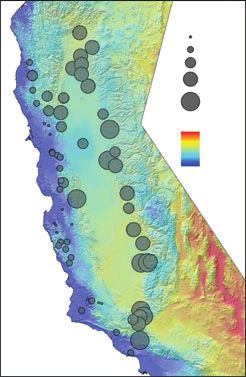
G E N E – C L I M A T E A S S O C I A T I O N S I N A C A L I F O R N I A O A K 3807

Overpeck 2000; Davis et al. 2005; Savolainen et al. 2007;        association between genetic and environmental gradi-
Aitken et al. 2008). Rapid environmental change, such            ents has been well established as evidence of natural
as occurred during the most recent-interglacial period           selection (Endler 1986; Mitton 1997; Manel et al. 2010).
of rapid warming, probably caused the extinction of              Forest genetics studies have shown that environmental
some tree species, but it is also possible that some pop-        heterogeneity influences the genetic differentiation
ulations survived those changes because local climates           among tree populations, creating geographic genetic
remained within the species physiological tolerance lim-         patterns that are consistent with phenotypic traits (see
its (Bennett 1997). Furthermore, as Davis et al. (2005)          Savolainen et al. 2007). One can look at this association
point out, evolutionary responses of local populations           to detect climate variables that are shaping the genetic
will include changes in the ability to migrate to and tol-       structure of populations (e.g. Foll & Gaggiotti 2006) or
erate new sites. Thus, range shifts related to major past        even identify which genes are under pronounced natu-
climate change have involved the interplay of dispersal          ral selection (e.g.Jump et al. 2006; Joost et al. 2008). If
and adaptive evolutionary responses. At issue is                 we are trying to understand the potential impact of
whether contemporary species can respond to the very             climate change, analysing the genetic structure of popu-
rapid rates of ongoing climate change.                           lations overlaid on current and future climate gradients
   Populations in different parts of a species’ range and        could help identify tree populations that are put at
in different microhabitats will experience and respond           greatest risk by rapid climate change.
to climate change differently (Rehfeldt et al. 2002, 2006).         Evaluating species–climate relationships and assess-
This differential response is due to both the genetic            ing impacts of climate change requires the use of rela-
composition of local populations and the magnitude of            tively fine-grained climate grids over large areas. High
climate change, which will vary geographically as well.          spatial resolution is especially important in mountain-
Some populations could remain under tolerable climatic           ous and coastal regions where climates vary widely
conditions while others will experience unsuitable               over short distances. In recent years climatologists have
climates. Furthermore, in areas with steep spatial               developed downscaling methods that incorporate infor-
climatic gradients range adjustments could occur over            mation on topography and marine influences to
relatively short distances compared to more uniform              improve high-resolution climate grids produced from
regions (Loarie et al. 2009), although potential migration       sparse station data or from coarse global climate models
rates will be highly sensitive to habitat fragmentation in       (Daly et al. 2008). These 800–1000 m resolution grids
the landscape (Ledig 1992; Holsinger 1993; Young et al.          have helped advance understanding of species–climate
1996; Bawa & Dayanandan 1998; Sork & Smouse 2006).               association and vulnerability to projected 21st century
Thus, understanding tree species’ responses to modern            climate change. However, for many regions where local
climate change will require better knowledge of geo-             populations may experience climatic conditions on a
graphic patterns of climate adaptation. These geograph-          smaller scale, such as rugged areas, even finer spatial
ical patterns have been shaped by a combination                  resolution may be needed to represent biologically
of isolation by distance, genetic drift, and selection by        important climate variation (e.g.Trivedi et al. 2008;
climate, along with other factors. Some local popula-            Randin et al. 2009).
tions may have tremendous phenotypic plasticity that                The motivation of this paper is to understand the
would allow tolerance to change, some may have suffi-            potential response of valley oak (Quercus lobata Née), a
cient genetic variation that will allow the next genera-         widely distributed California endemic tree species, to
tion of trees to respond to change through natural               climate change by exploring the associations of genetic
selection (Hamrick 2004), and others may have neither.           variation with locally resolved climatic variables. Valley
Spatial variation in genetic composition relative to             oak is an ecologically important tree species in Califor-
vagility will be pivotal to the ability of tree populations      nia that warrants evolutionary and conservation atten-
to respond to rapid climate change. For most tree spe-           tion. This oak has experienced extensive habitat loss
cies, identifying this variation is hampered by a lack of        (Kelly et al. 2005; Whipple et al. 2010), exacerbating the
common garden experiments and other more definitive              impacts of ongoing environmental change (Sork et al.
methods to identify local adaptation to climate (Davis           2009). Kueppers et al. (2005) predicted that the suitable
et al. 2005; Manel et al. 2010).                                 habitat for Quercus lobata will shift to favorable sites of
   Landscape genetics offers a range of spatial methods          higher latitude and elevation. Like nearly all climate-
for studying the influence of ecological processes on            based species distribution models, their models assume
genetic variation (Manel et al. 2003, 2010; Storfer et al.       that a single species–climate relationship can be applied
2007). Spatially explicit genetic and environmental              throughout the range. However, provenance studies
information can be used to look for the impacts of selec-        for many other species have documented systematic
tion (Manel et al. 2003; Storfer et al. 2007), and the           intraspecific variation in climate responses over tens to

! 2010 Blackwell Publishing Ltd
3808 V . L . S O R K E T A L .
thousands of kilometers (Aitken et al. 2008). In an ear-
lier study of valley oak (Grivet et al. 2008), we observed
a high degree of nuclear genetic variation across longi-
tude, latitude, and elevation, which suggests that popu-
lations across the species’ range will not respond
similarly to climate change.
Here, we address three objectives. First, to under-
stand the extent to which genetic lineages may con-
tribute to the genetic footprint of contemporary
populations, we examine historical patterns of coloni-
zation. Using maternally inherited chloroplast geno-
types of Quercus lobata, we examine range-wide
connectivity that has resulted from seed movement by
constructing population networks. Second, to assess the
extent to which current populations are climatically
structured in ways that may influence their response to
climate change, we examine the correlation between
multivariate nuclear genetic variation and climatic vari-
ation using canonical correlation analysis. Our genetic
analysis first transforms microsatellite markers, which
behave in a neutral manner as single loci, into multi-
variate genotypes that provide a sensitive measure of
genetic differentiation due to the combined effects of
gene flow, genetic drift, and selection across loci
(Smouse & Williams 1982; Westfall & Conkle 1992;
Zanetto et al. 1994). Third, to explore variation in
predicted 21st century spatial displacement of climate
zones across the species’ range of valley oak, we
parameterize region-specific species distribution models
using downscaled grids of historical climate and
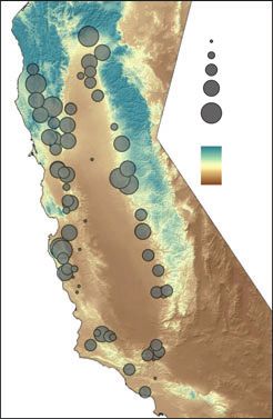
outputs from two climate models based on a moderate- Fig. 1 Map of species range of Quercus lobata (shaded area)
high carbon emission scenario. based on the California GAP Analysis database (Davis et al.
1998) and 80 sampling locations showing sites with nuclear
genotypes (dots) and sites with chloroplast genotypes (circles).
Materials and methods
distance dispersal (Smouse et al. 2001; Sork et al. 2002b;
Study species and study area
Pluess et al. 2009). However, these same populations
Quercus lobata (Née) is a dominant or co-dominant also have a fat-tailed dispersal kernel that indicates long
species in oak savannas, oak woodlands and riparian distance dispersal as well (Austerlitz et al. 2004; Pluess
forests across the foothills of the Sierra Nevada, Coastal et al. 2009). Acorns mature in late September to early
Ranges, and Transverse Ranges that surround the Cen- November of the year of pollination. Acorns lack
tral Valley of California (Griffin & Critchfield 1972; enforced dormancy and typically germinate within
Fig. 1). The species is winter-deciduous, phreatophytic, 1–2 months after maturation. Dispersal by birds and
and associated with deep loamy soils. This species has rodents typically results in movement of seeds less than
an extended latitudinal distribution (34–40" latitude) 150 m (Grivet et al. 2005; Scofield et al. 2010). Fine-scale
and altitudinal range (from sea level to 1700 m) result- genetic analysis of adults within a !230-ha area indi-
ing in Q. lobata populations that are spread across cates isolation by distance at !350 m (r) for seed and
diverse climatic and geographical zones. pollen together (Dutech et al. 2005). These studies of
Gene movement occurs through wind-pollination and local historical and contemporary gene flow indicate
the mating system is predominantly outcrossing (Sork that the scale of dispersal is on the range of 100–300 m,
et al. 2002a). In estimates of contemporary gene flow which allows for the opportunity for adaptation to local
through pollen, average pollen dispersal distance com- environmental conditions. Grivet et al. (2006) report
puted with indirect and direct approaches yielded an regional scale of spatial autocorrelation in chloroplast
estimate of 65–114 m, with a high propensity for short genotypes up to 100 km.
! 2010 Blackwell Publishing LtdG E N E – C L I M A T E A S S O C I A T I O N S I N A C A L I F O R N I A O A K 3809
chi-squared test (Garrick et al. 2009). PopGraph also
Sampling
identifies pairs of populations that are located signifi-
From 2003 through 2009, we sampled 330 Q. lobata indi- cantly closer than predicted by inter-site separation,
viduals from 80 sites throughout the species range which suggests that a direct barrier might exist between
(Fig. 1), as part of an ongoing project on the phylogeog- the linear distances. We conducted analyses through
raphy and conservation of California oaks (Grivet et al. the online version of Genetic Studio (http://www.dyer-
2006, 2008; Sork et al. 2009). For this study, our sample lab.vmu/software) to create the topology, and then
sizes include 190 chloroplast microsatellite haplotypes viewed the population graph with a downloadable
across 64 sites and 267 nuclear genotypes across 65 version of Graph (Dyer 2009). We plotted the geographi-
sites. The two data sets share 44 sites, and each samples cal patterns using ArcMap 9.2 (ESRI Inc).
the full species’ range.
Climate data set. Grids of historical climate were pro-
duced by downscaling monthly 4 km PRISM climate
DNA extraction and genotyping
data (Daly et al. 2008) for the period 1971–2000. Down-
For the additional samples collected since our previous scaling was accomplished with 90 m digital elevation
publications (Grivet et al. 2006, 2008; Sork et al. 2009), grids using a modified gradient-inverse-distance square
we analysed six chloroplast microsatellite genetic mark- interpolation method (Flint & Flint 2007, 2010). The
ers (Deguilloux et al. 2003) using the same DNA extrac- method preserves the structure of the coarser PRISM
tion method and PCR conditions. For the new samples grids and uses 90 m digital elevation data for additional
and a subset of earlier samples, we measured the length downscaling. Flint & Flint (2010) analysed predicted
of the amplified sequence by running an aliquot of each and observed air temperatures at more than 130 Califor-
PCR product on an ABI 3700 capillary sequencer at the nia Irrigation and Management Information System
UCLA Sequencing & Genotyping Core Facility (http:// (CIMIS) stations and 80 National Weather Service
www.genetics.ucla.edu/sequencing/index.php). The stations in the rugged central Sierra Nevada to deter-
two methods were calibrated to ensure that we mine the reliability of downscaling from the 4 km
assigned the same haplotypes across primers. PRISM cells to 90 m for California. They determined
The nuclear data set, which also augmented previous that there was little if any bias for air temperature and
samples, was genotyped using the same methods that the errors were the same in coastal as interior Cali-
described elsewhere (Grivet et al. 2008; Pluess et al. fornia. The downscaling algorithm either had no influ-
2009) for six nuclear microsatellite primers: MSQ4, ence or improved interpolated estimates of temperature
QpZAG1 ⁄ 5, QpZAG9, QpZAG36, QpZAG110, and regimes at the validation sites.
QrZAG20. To verify repeatability, each sample was We derived mean values from downscaled climate
re-genotyped after repeating the PCR reactions. Again, grids for the periods 1971–2000 and 2070–2100. We
we reran a subsample of previously genotyped individ- analysed mean annual precipitation and several temper-
uals to ensure consistency in genotype assignments. ature variables expected to be physiologically relevant
and shown to be important in other studies of western
Data analyses tree distributions (Rehfeldt et al. 2006), including mini-
mum temperature of the coldest month (Tmin), maxi-
Chloroplast genotypes. To understand the extent to which mum temperature of the warmest month (Tmax),
seed movement has dispersed genes across the species temperature seasonality (Tseas), and annual growing
range, we analysed the maternally inherited chloroplast degree days above 5"C (GDD5):
genotypes through PopGraph (Dyer & Nason 2004;
Garrick et al. 2009) to create a network of connections
12 #!
X " $
among sites. This software uses a graph-theoretical T mini þT maxi
GDD5 ¼ $ 5 Di
approach and analyses how genetic variation is distrib- i¼1
2
uted across the landscape. The software creates nodes
based on the genetic variation within sites and identi- where Tmin and Tmax are average minimum and maxi-
fies a network of connections among sites based on mum temperatures for month i and D is the number of
genetic covariation among all populations estimated days in month i. When Tmini < 5"C < Tmaxi, we adjust
simultaneously conditional on the entire data set. the number of days in the month using D* =
PopGraph identifies pairs of populations where long D(Tmax ) 5) ⁄ (Tmax ) Tmin). Temperature seasonality
distance migration may have occurred by indicating was calculated as the standard deviation of monthly
population pairs with significantly greater inter-site dis- mean temperatures rescaled from 0 to 100 for the range
tances than predicted by spatial separation based on a of values observed in California. The climate variables
! 2010 Blackwell Publishing Ltd3810 V . L . S O R K E T A L .
Table 1 Pearson’s correlation coefficients of latitude and longitude spatial coordinates, and seven climate variables based on the
90 m resolution grids produced by downscaling of daily 800 m PRISM climate data (Daly et al. 2008)
X Y GDD5 Tmax Tmin MAP
East–west (X) 1.000
North–south (Y) )0.585 1.000
Growing degree days (GDD5) 0.430 )0.056 1.000
Monthly maximum temperature (Tmax) 0.370 0.054 0.654 1.000
Monthly minimum temperature (Tmin) )0.009 0.074 0.435 )0.334 1.000
Mean annual precipitation (MAP) )0.499 0.684 )0.447 )0.232 )0.079 1.000
Temperature seasonality (Tseas) 0.533 0.167 0.467 0.709 )0.154 )0.095
are correlated with longitude (X) and latitude (Y) as small number of linear combinations from each set that
well as with each other (Table 1). have the highest possible between-set correlations
Downscaled global climate model (GCM) predictions (Legendre & Legendre 1998). Using the PROC CANCORR
for the period 2070–2100 were produced by downscal- function of SAS (SAS Institute 1989), we analysed the
ing aggregated monthly outputs for the period correlation between multivariate genotypic scores from
2070–2100 from the Parallel Climate Model (PCM1, the first 20 axes with five of the climate variables
developed by the National Center for Atmospheric described above. To incorporate nonlinear structure in
Research and the Department of Energy) and the God- the climate variables, we used canonical trend surface
dard Fluid Dynamics Laboratory (GFDL) climate model. analysis, which also includes squared terms and cross
Downscaling involved initial downscaling of coarse products among the five variables, which yielded a total
PCM1 output using the constructed analogue method of 20 climate variables. We tested the normality of
(Hidalgo et al. 2008). We are using a moderately high residuals of the canonical models using SAS PROC UNIVARI-
21st Century carbon emission scenario (A2). The PCM- ATE. To diagnostically describe the forms of the equa-
A2 and GFDL-A2 scenarios are two of four selected by tions (Box & Draper 1987), we analysed the observed
the State of California for assessing climate change scores for the first four canonical axes in SAS PROC RSREG.
impacts, the others being PCM1 and GFDL with the This procedure uses the method of least squares to fit
lower B1 emission scenario (Cayan et al. 2008). Com- quadratic response surface regression models and trans-
pared to the GFDL-A2 model runs, PCM1-A2 predicts forms that model to describe the shape of the response
lower late-century temperature increase (2.6"C vs. 4.5"C surface.
mean statewide annual temperature) and smaller differ- To assess the contribution of geography to the canoni-
ences in precipitation (e.g. )2% vs. )18% change in cal correlation model, we partitioned out the spatial
statewide mean annual precipitation). component of the climatic variation (Borcard et al.
1992), which was done in two steps. In the first step,
Nuclear genotype data set. We used principal component using stepwise or sequential (Type I) sums of squares,
analysis (PCA) to reduce dimensionality in the micro- we specified a quadratic model of geographic coordi-
satellite allelic variables and create multivariate genetic nates (x, y, and elevation, in metres) first, then the
variables in the same manner as described in Grivet climatic model. In the second step, we specified the cli-
et al. (2008). First, we transformed single locus geno- matic model first, followed by the geographic model. In
types into allelic variables by assigning a score of 0, 0.5, the first model, we have the proportion of the total
or 1, depending on whether the individual possesses a sums of squares due to climate after removing geogra-
homozygous or heterozygous alleles at that locus (West- phy; in the second, we have that proportion due to
fall & Conkle 1992). The number of single variables cre- geography after removing that due to climate. From
ated at each locus is the number of alleles minus one, these, we can compute the proportion of total sums of
which yielded 102 allelic variables. We then use PROC squares that is collinear.
PRINCOM in SAS (SAS Institute 1989) to reduce the 102
variables into a smaller set of orthogonal axes.
Modelling of future shifts in climate zones
Climate associations of genotypes. To test the relationship To explore the extent to potential for spatial displace-
between genetic variation and climate, we conducted a ment of historical regional climates in the near future,
canonical correlation analysis, which summarizes the we selected four sampling sites that were evenly dis-
relationship between two sets of variables by finding a tributed throughout the range of valley oak and also
! 2010 Blackwell Publishing LtdG E N E – C L I M A T E A S S O C I A T I O N S I N A C A L I F O R N I A O A K 3811
spanned the range of genetic dissimilarity. A circular
buffer with a radius of 75 km was created around each
site.
We combined valley oak location information from
our samples with occurrence data from a database of
California vegetation plots (Seo et al. 2009) to generate
a presence-only database of 529 valley oak locations
that fell within the 4 subregions. Species distribution
models were created using maximum entropy (MAXENT
version 3.1.0) modelling (Phillips et al. 2006; Phillips &
Dudı¢k 2008) with mean annual precipitation, tempera-
ture seasonality and growing degree days above 5". The
MAXENT approach has proven to be very effective for
bioclimatic modelling and performs better with pres-
ence-only data than most other available methods (Elith
et al. 2006). Separate MAXENT models were produced
based on nonoverlapping occurrence data in each of the
four subregions. Model goodness-of-fit was evaluated
using the area under the receiver operating characteris-
tics curve (AUC).
To map late 21st Century distributions, each regional
model produced using historical climate data was
applied to state-wide grids of predicted future climate.
Fig. 2 Map of network showing 64 sites that are significantly
To simplify presentation of the results, we show pre- connected with each other based on PopGraph topology (see
dicted presence or absence rather than probabilities text for details). Sites that are spatially more distant than
using a threshold of P = 0.5 for species presence (Phil- expected from their genetic differences indicate long distance
lips & Dudı¢k 2008). dispersal (white lines) and those that are spatially closer than
expected from genetic differences indicate barriers (white
dashed lines).
Results
Both genetic markers included high genetic diversity. tivity among most populations (Fig. 2). The most
The chloroplast results indicate that Quercus lobata is var- common colonization patterns are north and south
iable across the six microsatellite markers with 2–5 hapl- along the foothills of both the Coast Ranges and Sierra
otypes per marker with an overall average of 3.9 Nevada, but it is not uncommon to see east–west gene
haplotypes, and a total of 45 unique multilocus haplo- exchanges, especially in the northern part of the species
types across the 64 sites and 190 individuals (see range. Our data indicate occasional long distance gene
Table S1, Supporting information). The nuclear genetic exchange across the Central valley from the coastal
diversity is greater than that of chloroplast, which is northern site to an eastern southern site where the hapl-
expected. The total number of alleles per nuclear micro- otypes are significantly more similar than expected
satellite locus ranged from 10 to 29 alleles, with an aver- based on spatial distance. Our analysis also identifies a
age of 18 alleles across loci (see Table S1, Supporting network connection across the Central valley in south-
information). The range of the average effective number ern California where the two sites are more genetically
of alleles per site was 2.5–4.7 alleles. The average num- dissimilar than predicted by spatial distance.
ber of alleles per site ranged from 2.9 to 5.5, which is
fairly high given that most sites included only three indi-
Climate associations of genotypes
viduals, and thus could not exceed 6 alleles per locus
per site. We did not adjust these averages for sample size We used the multivariate scores from the first 20 princi-
because the data are presented as background informa- pal component axes as multivariate genotypes for the
tion and not for future statistical analysis. canonical correlation analysis. We chose 20 PC’s
because this number captured a reasonable amount of
the total genetic variation (the cumulative percentage
Chloroplast genetic networks
was 41.52%, Table 2), and use of additional PC’s
The PopGraph network of populations based on chloro- improved the R2s in the subsequent correlation analysis
plast haplotypes indicates extensive historical connec- marginally. The proportion of genetic variation attributed
! 2010 Blackwell Publishing Ltd3812 V . L . S O R K E T A L .
Table 2 Eigenvalues of the Principal Component Axes (PCA) Table 3 Summary of Canonical Correlation Analysis based on
from the PC correlation matrix based on 103 allelic variables nuclear microsatelite genetic markers. (A) Summary of the sta-
from 7 nuclear microsatellite loci tistical tests of canonical correlation analysis for genetic vari-
ables vs. six climate variables, their quadratic forms, and their
Prin Eigenvalue Proportion Cumulative cross products. (B) Canonical correlations of the 20 PCAs of
the 103 nuclear variables with the observed scores of the first
Prin1 3.71933157 0.0365 0.0365 four canonical axes. (C) Canonical correlations of the linear
Prin2 3.04415982 0.0298 0.0663 and higher order combinations of the climate variables for the
Prin3 2.54074113 0.0249 0.0912 first four canonical axes
Prin4 2.43914075 0.0239 0.1151
Prin5 2.32291626 0.0228 0.1379 Canonical axes Canonical correlation Pr > F
Prin6 2.23144517 0.0219 0.1598
Prin7 2.18288316 0.0214 0.1812 (A) Statistical tests for first six canonical axes
Prin8 2.09034455 0.0205 0.2017 1 0.765617G E N E – C L I M A T E A S S O C I A T I O N S I N A C A L I F O R N I A O A K 3813
Table 3 (Continued) terns. So that the stationary point is outside the data in
CV3 is not unexpected. In CV4, there is little spatial
Climate variable W1 W2 W3 W4 association in plotted scores (not shown), which is indi-
cated by the low collinearity with geography (next par-
GDD5 · MAP 0.2440 0.1264 0.4703 )0.3596
GDD5 · Tmax )0.2744 0.4409 )0.3152 )0.0186 agraph) and low correlations with climate. Instead, the
GDD5 · Tmin )0.0387 0.1410 )0.1146 )0.1595 low (albeit significant) association we did find was due
GDD5 · Tseas )0.2234 0.6875 )0.1033 0.1108 to a few extreme values in the scores. This pattern sug-
MAP · Tmax 0.2651 0.1032 0.4958 )0.3047 gests that trends in CV4 could be due to drift, rather
MAP · Tmin 0.1123 0.0118 0.0811 )0.3016 than an influence of climate.
MAP · Tseas 0.1471 0.4277 0.4098 )0.0962 Our analysis of the collinearity between climate and
Tmax · Tmin 0.0097 0.1832 )0.1115 )0.1927
spatial location indicated that 34% of the sums of
Tmax · Tseas )0.2084 0.6674 )0.0393 0.1584
Tmin · Tseas 0.0970 0.4246 )0.1157 )0.1305 squares (SS) for the first canonical axis were due to cli-
mate alone and 52% of the association between genetic
and climate variation was due to the collinearity of cli-
variables in its linear, quadratic, and cross product mate and geography. In the second canonical axis, 43%
forms. In the third vector (W3), mean annual precipita- of the SS was due to climate alone and 43% was due to
tion (MAP) was highly correlated in their linear, qua- collinearity with geography. In the third axis, 56% of SS
dratic, and cross-product forms. In the fourth vector was due to climate alone and 25% was due to the col-
(W4), MAP is highly correlated. Overall, all of the vec- linearity. In the fourth axis, 78% was due to climate
tors are correlated with more than one climate variable alone and 4% due to collinearity.
in linear and higher order forms, but GDD5, Tseas, and To illustrate the spatial patterns in genetic and cli-
MAP, were the strongest climate variables for the first mate variables, we plotted the predicted canonical
three canonical vectors, respectively. The residuals of scores for the first three axes onto three climate gradi-
the model for the first four canonical scores were nor- ents for GDD5, Tseas, and MAP, respectively. Because
mally distributed. the scores are based on all five climate variables, we
The RSREG procedure analysed the canonical trend would not expect that the scores would precisely corre-
surface for the first four canonical vectors (CV), and spond to the temperate gradients, but these maps illus-
confirmed both that large proportions of variation in trate the trend in the data. Figure 3A illustrates the
the models were nonlinear and also that substantial southern Sierra Nevada foothills and northern Sacra-
proportions were due to interactions among climate mento Valley experience higher growing degree day
variables (Table 4). The forms of all models were sad- sums than those sums elsewhere in the species’ range
dles, where, from the middle (or stationary point), (Fig. 3A). The canonical scores associated with the first
canonical scores rose or fell, moving off the stationary axis (CCA1) were smaller in the areas in the southern
point. So depending on the signs of the relationships Sierra Nevada foothills and very southern California.
with each CV, PC scores rose or fell, as did frequencies Temperature seasonality (Fig. 3B) is lower in the sites
of alleles associated with each PC, with variation in the along the Coastal range foothills than along the Sierra-
CV. In the first two CVs, the stationary point was Nevada foothills, and here we see smaller canonical
within the range of the climate data, whereas that point scores of the second axis (CCA2) located in the coastal
was outside the range of the data in CV3, representing area with low seasonality. Mean annual precipitation
a climate outside our data. Spatial patterns in precipita- shows north south gradient (Fig. 3C), and the smaller
tion are complex, not only dependent on orographic CCA3 scores tend to be in areas with very little precipi-
effects, but also on large-scale and local circulation pat- tation.
Table 4 Summary of Type I statistics from separate response surface regression models for scores of the four canonical axes of the
CTSA reported in Table 3
V1 V2 V3 V4
DF R2 Pr > F R2 Pr > F R2 Pr > F R2 Pr > F
Linear 5 0.23963814 V . L . S O R K E T A L .
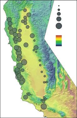
(A) (B) (C)
Fig. 3 Overlay of predicted canonical scores onto map of climate gradients. (A) Observed canonical scores for first vector (V1) vs.
growing degree days (GDD5). (B) Observed canonical scores for second vector (V2) vs. Temperature Seasonality (Tseas). (C)
Observed canonical scores for third vector (V3) vs. precipitation.
Future shifts in climate zones increases. Both scenarios predict greatest warming in
the southern and western subregions. Temperature sea-
Valley oaks occur in systematically different climates
sonality is also predicted to increase in all regions,
within the four test regions that span north–south
although the GFDL-A2 model predicts much larger
and east–west extremes in the range (Table 5). The
increases. The models differ considerably in precipita-
northern region and central Sierran foothill locations
tion forecasts: the GFDL-A2 scenario predicts drier con-
are generally wetter than locations in the southern
ditions in all four regions (more pronounced in the
range or the Central Coast. Northern sites experience
North and East) while the PCM1-A2 scenario includes
lower GDD5 values while the central coastal and
modest increases in precipitation in all regions (less
southern sites experience much lower temperature
pronounced in the West; Table 5).
seasonality.
MAXENT models based on training data from the
Both GFDL-A2 and PCM1-A2 climate scenarios pre-
separate regions all have high values for model fit
dict large increases in GDD5 at all 4 test regions,
(AUC values ‡0.95) (Table 6). MAP contributes more
although the GFDL-A2 forecasts consistently greater
Table 5 Summary of downscaled climate values for valley oak localities in 4 circular regions 150 km in diameter within the current
range. The number of nonoverlapping sites varies from 47 in the northernmost region to 198 in the southernmost region. Means and
standard deviations are for the period 1971–2000. The values of DGFDL-A2 and DPCM-A2 are the differences of climate means for
the period 2071–2100 minus the means for the period 1971–2000. Variables include mean annual precipitation in mm (MAP), temper-
ature seasonality (the standard deviation of monthly mean temperatures, rescaled from 0 to 100 for minimum and maximum values
in California), and growing degree days above 5" in "C (see text for explanation)
MAP Tseas GDD5
No. of
Region sites Mean SD DGFDL-A2 DPCM-A2 Mean SD DGFDL-A2 DPCM-A2 Mean SD DGFDL-A2 DPCM-A2
North 138 766 173 )286 65 44 3 9 2 3365 583 1325 1096
East 47 874 232 )238 63 44 3 11 3 4058 298 1317 1069
West 198 439 64 )170 25 28 13 6 2 3959 736 1457 1159
South 146 535 128 )123 60 30 8 10 1 3880 263 1494 1201
! 2010 Blackwell Publishing LtdG E N E – C L I M A T E A S S O C I A T I O N S I N A C A L I F O R N I A O A K 3815
Table 6 Summary of model fit (AUC, Area under the Receiver across the range. Thus, seed movement, when com-
Operator Characteristics curve) and climate variable contribu- bined with gene flow through pollen movement, has
tions for four climate-based species distribution models based resulted in continuously distributed genetic variation
on the Maximum Entropy (MAXENT) method
with a modest amount of nuclear geographic structure
Variable contributions (%) (Grivet et al. 2008). In this paper, we find that nuclear
multilocus genetic structure shows a strong association
Region N AUC MAP Tseas GDD5 with climatic gradients. This climatically associated
genetic structure provides the opportunity for local
North 138 0.991 49.5 11.4 39.1 adaptation to climate and may influence the response of
East 47 0.946 52.8 19.7 27.5
local populations to future climate change.
West 198 0.987 18.8 44.1 37.1
South 146 0.983 42.4 32.9 24.9
Historical seed movement in Valley oak
The historical movement of valley oak over its evolu-
than Tseas or GDD5 in three of the models but temper- tionary history appears to have been sufficient to allow
ature variables contribute significantly to all models, gene exchange across its range. Valley oak has a rela-
especially the model for the western coastal region. tively large amount of haplotype diversity, especially
The predicted temperature changes lead to larger when contrasted with the European white oaks sampled
spatial shifts of suitable climate zones in some regions on a similar spatial scale and genotyped with the same
than others (Fig. 4). Climates similar to occupied sites markers (Grivet et al. 2006). This contrast in haplotype
in the western coastal region are predicted to be greatly diversity with European populations provides evidence
reduced in extent (PCM-A2, Fig. 4b) or occur only in that contemporary valley oak populations are older
limited areas more than 100 km distant from current than the occurrence of the Last Glacial maxima. The
sites and nearer to the coast (GFDL-A2, Fig. 4a). lack of recent glaciation in California would have
Climatically suitable areas for trees in the northern allowed populations to survive cold periods in multiple
region are predicted to expand greatly into surrounding regions and retain their diversity. During the warm
foothill regions and highly suitable areas either partially and cool periods of the Pleistocene, as populations
overlap (GFDL-A2, Fig. 4c) or fully overlap with expanded and contracted, they would have had ample
currently occupied sites (PCM1-A2, Fig. 4d). For inte- opportunity to disperse and colonize many sites in
rior sites currently located in the foothills of the Sierra California.
Nevada, comparable climates are predicted to have The network analysis of the chloroplast haplotypes
little overlap with current sites but to shift locally demonstrates extensive gene movement through coloni-
upslope within 1–20 km of currently suitable climate zation. North ⁄ south movement along the foothills of the
locations (Fig. 4e,f). At the southern end of the range, Coastal and Sierra Nevada Ranges seems particularly
areas of suitable climate comparable to currently occu- common. In the northern part of valley oak distribution,
pied sites occur locally at higher elevations within a we see several connections across the Central Valley
few km of currently occupied sites as well as at distant probably due to a strong riparian network (Grivet et al.
sites (Fig. 4g,h). 2008). In the southern part, long distance connectivity
occurred from northwest to southeast, but it is difficult
to distinguish whether the long distant events actually
Discussion
crossed the Central Valley diagonally or they moved in
The ability of a species to persist under the conditions a stepping stone fashion across the northern Central
of rapid climate change will be determined by the Valley and then south along the foothills. The pattern
responses of local populations (Jackson & Overpeck of the population network suggests that the western
2000; Davis & Shaw 2001; Davis et al. 2005; Aitken et al. region about the San Francisco Bay area may be a
2008). Will they be able to tolerate or adapt to changes source region. In the south, we observed occasional
in local conditions? Will they be able to track shifts in east–west linkages across the southern Central valley,
climate zones? Or, will they go extinct? Despite the fact but with much less frequency. In one case, the inter-
that chloroplast markers show strong geographic struc- population genetic distance is significantly further than
ture (Grivet et al. 2008), here we show that historical predicted by inter-site physical distance, which implies
seed movement of valley oak includes long distance that those haplotypes may have taken an indirect route
colonization events. These events are mostly north and to arrive in the Sierra Nevada foothills.
south, but we also observe east–west colonization that The movement of seeds across the range would also
would have included the dispersal of nuclear genotypes have homogenized the nuclear genetic variation to
! 2010 Blackwell Publishing Ltd3816 V . L . S O R K E T A L .
some extent. Moreover, given that gene flow in this These geographic patterns of climatically structured
species is even greater through pollen than seeds genetic variation may provide a useful indication of
(Grivet et al. 2009a; Pluess et al. 2009), pollen-mediated the geographic patterns of adaptive variation. They
gene movement should have also promoted gene could have been shaped by selection on genes that
exchange throughout the species range. We point out are linked to the markers due to genetic hitchhiking
that the reduced seed movement across the southern (Barton 2000) or selective sweeps associated with poly-
Central valley between east and western populations genic traits (Pritchard et al. 2010). Recent work using
would allow vicariance to contribute to the geogra- genome scans to identify the association of AFLP loci
phical genetic differences between those two regions. with environmental gradients illustrates that selection
Future analyses can utilize models that will allow the can influence putatively neutral genetic variation
separate contributions of phylogeographic structure and through these processes (e.g. Freedman et al. 2010;
environmental variables that could help sort out the Thomassen et al. 2010). Of course, isolation by distance
contribution of vicariance (Dyer et al. 2010). Nonethe- and genetic drift could also shape geographic struc-
less, we observe enough gene movement to deduce ture, but the correlation with environmental gradients
that the patterns of geographic structure we discuss indicates an influence of selection. In our study, we
below cannot be solely attributed to restricted gene see evidence for the influence of selection when we
movement. examine colinearity between genetic variation, climate
variation, and geography. Even when we partition out
the effect of spatial location, genetic variation is
Association of nuclear genetic variation with climatic
strongly associated with climatic variation. While
variables
vicariance may contribute to the significance of the
Multivariate genetic variation in valley oak is signifi- first canonical vector, the second and third canonical
cantly correlated with multivariate climatic variation. It vectors provide evidence for the role of selection.
may seem paradoxical that markers such as nuclear mi- Thus, the genetic structure of our populations illus-
crosatellites, which are putatively neutral as single loci, trates the opportunity for adaptation to local climate
would show an association with climate; however, and allows the formulation of hypotheses and identifi-
selection is not acting on these loci per se, but rather on cation of appropriate spatial scales for additional sam-
the whole genotype. The accumulation of small effects pling. In the future, a landscape genomic approach,
across loci, especially linked loci, due to selection, along especially using candidate genes related to response to
with gene flow and drift, creates a relatively sensitive climate, will be a more direct way to identify geo-
measure of genetic differences among populations. The graphic patterns of adaptive variation (Eckert et al.
most conspicuous difference was between the eastern 2010; Manel et al. 2010; Thomassen et al. 2010).
and western parts of the species range. However, for
some of the canonical axes, those east–west differences
Regional variation in distribution models under
are as strong in the northern part of the species range
current and future climates
where connectivity is relatively high as in the southern
part where the connectivity is less. Scores for the first Maxent models based on mean annual precipitation,
canonical axis, which is most correlated with growing temperature seasonality and growing degree days pro-
degree days, are highest in the central-western part of vide good fits to observation data, with AUC values
the range and the scores are lowest in the south and ranging from 0.95 to 0.99 for the different subregions.
south eastern part of the range. Second axis scores, Consistent with theory (Davis et al. 2005) and empirical
which are highly correlated with temperature seasonali- evidence (Rehfeldt et al. 2002), populations in different
ty, reveal genetic differentiation between populations in portions of the range experience systematically different
the Coast Range foothills vs. eastern populations adjoin- climate regimes, so that climate models fitted to obser-
ing the Sierra Nevada. For the third canonical axis, pre- vations in one subregion have lower accuracy predict-
cipitation is a key climate variable, both linearly and in ing the occurrence of valley oaks in more distant
quadratic form. subregions (Fig. 4).
Fig. 4 Maps of climate-based species distribution models fitted using MAXENT and parameterized using locality data from each of
four circled areas. Models were fitted using downscaled grids of mean annual precipitation (MAP), growing degree days above 5
degrees (GDD5), and temperature seasonality (Tseas) for the period 1971–2000. Black areas have probability of occurrence values
exceeding 0.5. Gray areas are extrapolated distributions (P > 0.5) based on the same regional climate model but using climate fore-
casts based on GFDL-A2 (a, c, e, g) and PCM-A2 (b, d, f, h) models for the period 2071–2100. Dark gray areas are where P > 0.5 in
both current and future models.
! 2010 Blackwell Publishing LtdG E N E – C L I M A T E A S S O C I A T I O N S I N A C A L I F O R N I A O A K 3817 (a) (b) (c) (d) ! 2010 Blackwell Publishing Ltd
3818 V . L . S O R K E T A L .

(e)                              (f)

(g)                              (h)

Fig. 4 (Continued)

                                       ! 2010 Blackwell Publishing Ltd
G E N E – C L I M A T E A S S O C I A T I O N S I N A C A L I F O R N I A O A K 3819
The strong spatial structure of genetic variation tion (Tyler et al. 2006). The survival of extant popula-
in valley oak and associated inter-regional variation in tions will require either an ability to adapt to new
climate-based distribution models suggest that valley climates or the presence of individuals that can tolerate
oak populations will experience region-specific climate the new conditions. As a species with relatively long
change impacts. The differences in the extent of climate generation time, adaptation is unlikely to be an effec-
displacement reflect both regional differences in the tive response. However, it is possible that local popula-
magnitude of projected climate change and the steep- tions might include individuals that can tolerate new
ness of local topographically induced temperature and conditions, which is especially likely for those popula-
precipitation gradients. Our results indicate that central tions in regions with variable climate conditions (e.g.
coastal populations are especially vulnerable because Sierra foothills). Our regional climate envelopes indi-
increases in temperature and seasonality are propor- cate that the three climate variables we examined con-
tionally greater here and shallower spatial climate gra- tribute differently across regions. For example, mean
dients equate to longer distances for range adjustments annual precipitation contributes most to the distribu-
than for populations elsewhere in the range (Loarie tion of valley oak in the east, north, and south regions
et al. 2009). (42–53%), but its contribution is small in the west
We recognize that interpolated climate grids are region (19%). In contrast, temperature seasonality is
imperfect models of actual local spatial variation and important in the west and south regions, but less so in
that such bioclimatic analyses would benefit from den- the North and East regions, where seasonality is actu-
ser climate station networks. Comparison to other ally very high (see Fig. 3B). As future climates in the
downscaling methods, such as nonparametric splines west become warmer and more seasonal, one can spec-
(Rehfeldt et al. 2006) and dynamic regional climate ulate whether existing populations have the plasticity
models (e.g. Kueppers et al. 2005) is also worth pursu- to tolerate this shift in climate. Our analysis would
ing. Furthermore, other environmental factors could suggest that western regional populations may be more
affect these results, notably local soil and hydrologic vulnerable to climate change than the eastern ones and
conditions. Valley oaks are associated with deep loamy that tolerance to climate change, in general, is going to
soils as well as valley floor and riparian sites with rela- be regionally dependent on the interaction between
tively high water tables. We are currently examining local genetic variation and climate conditions.
the interaction of soil factors and climate factors and
comparing different downscaling methods in regional
Implications for adaptive genetic variation
distribution models for the species.
Over a long evolutionary period, tree populations As we consider the vulnerability of populations to
have tremendous potential for gene flow through seeds respond to climate change, patterns of adaptive genetic
and pollen (Aitken et al. 2008). In our estimates of con- variation will be more critical than those of neutral
temporary pollen dispersal, the size of a genetic neigh- genetic variation (Holderegger et al. 2006). As a first
bourhood is on the scale of 100 m but with potential for step, it is useful to simply understand how geographic
rare long distant dispersal (Austerlitz et al. 2004; Pluess genetic structure is associated with climate variables so
et al. 2009) that could spread novel alleles for several to that we can make some first order approximations
tens of kilometres. Our studies of seed dispersal indi- about potential responses (Manel et al. 2010). Forest
cate very restricted dispersal, but here too occasional geneticists have used genetic markers in this way to
long distance dispersal events over a kilometre take construct seed zones to select genotypes for plantations
place (Sork et al. manuscript in preparation). For exam- (see Westfall & Conkle 1992). The microsatellite markers
ple, birds such as jays can regularly transport acorns examined in this study have described geographic
several kilometres and plant them in the soil (Gomez genetic structure, and revealed genetic clines associated
2003). Palaeoecological studies of eastern North Ameri- with geographical and climatic gradients. These clines
can oaks, based on recolonization after glaciations, esti- provide the opportunity for selection on phenotypic
mate that migration rates are about 100 m per year traits but whether these clines are correlated with adap-
(McLachlan & Clark 2004), or 6–8 km in 60–80 years, tive evolution has to be carefully demonstrated. Other
which is less than the climate zone shifts for many parts processes, such as migration or range expansion, may
of the valley oak range predicted by our models. Thus, generate such clines in loci across environmental gradi-
tracking climate change is probably not a likely scenario ents. After portioning out the effect of spatial location,
for many valley oak populations under the current we still find significant variation due to the genetic
rapid rates of climate change. association with climate. The next step would be to
The future of valley oak has many challenges such identify candidate genes associated with these traits
as regeneration difficulties and landscape transforma- and assess whether geographic variation in SNPs
! 2010 Blackwell Publishing Ltd3820 V . L . S O R K E T A L .
follows environmental gradients in a similar geographic ence particularly dramatic shifts in climate zones, the
pattern. underlying climatically based genetic structure may
Population genomics is facilitating the identification constrain the ability of populations to tolerate that rapid
of adaptive molecular variation by examining numerous climate change. Future studies using candidate genes
loci or genome regions, and recent advances in gen- and common garden experiments are needed to evalu-
ome-wide scans have allowed examining footprint of ate the extent to which spatially distributed local popu-
selection in numerous species (Luikart et al. 2003; Niel- lations can tolerate or adapt to future climate
sen 2005; Biwas & Akey 2006). One could take two conditions.
approaches. The first one would be to examine varia-
tion within candidate genes coding for known biologi-
Acknowledgements
cal functions, potentially correlated with adaptive traits,
such as phenology (Heuertz et al. 2006; Pyhajarvi et al. We thank the anonymous reviewers who provide valuable
2007), drought tolerance (González-Martı́nez et al. 2006; suggestions on how to improve the manuscript. We are grate-
Pyhajarvi et al. 2007; Eveno et al. 2008; Grivet et al. ful to: Rodney Dyer and Doug Scofield for discussions of
data analysis; Keith Gaddis, Karen Lundy, Stephanie Steele,
2009b) or cold resistance (Wachowiak et al. 2009). The
and Pam Thompson for comments on manuscript; Charles
second would use a random scan of the genome and Winder, Edith Martinez, and Karen Lundy for laboratory
look for loci or SNP potentially under selection (e.g. work; and Uma Dandekar and other staff at the UCLA
Namroud et al. 2008; Eckert et al. 2010). The next step Sequencing and Genotyping Core Facility. We thank all those
is to link SNP’s under selection with phenotypes mea- people who were drafted into collecting oak leaves, including
sured in common gardens through association studies Brian Alfaro, Maria Valbuena-Carabaña, Kurt Merg, Andrea
(e.g. González-Martı́nez et al. 2007). The geographic Pluess, Andrea Sork, Danielle Sork, Silke Werth, and Charles
Winder. Over the years of data collection and analysis, VLS
mapping of those SNP’s could then provide a direct
received funding from UCLA Division of Life Sciences, UCLA
indicator of how various populations have responded Senate Faculty Research Programme, NSF DEB-0089445, NSF
to past climate change and thus may respond to future DEB-0516529, and the National Geographic Society. FWD and
climate change. Currently, work is underway with val- MI were supported by California Energy Commission
ley oak to identify SNP variation at candidate genes research project CEC 500-08-020. HW was supported by the
linked to traits such as drought tolerance and phenol- China National Scientific and Technical Foundation Project
ogy, which would allow us to map adaptive variation (Grant No. 2006FY210100).
on the landscape and assess its association with climate
variables. References
Ultimately, intense genome scans linked with com-
mon garden measurements of phenotypes will allow us Aitken SN, Yeaman S, Holliday JA, Wang TL, Curtis-McLane S
(2008) Adaptation, migration or extirpation: climate change
to assess the extent to which the mapping of candidate
outcomes for tree populations. Evolutionary Applications, 1,
genetic variation provides insight about the ability of 95–111.
local populations to tolerate climate change. It is Austerlitz F, Dick CW, Dutech C et al. (2004) Using genetic
encouraging that studies have found associations markers to estimate the pollen dispersal curve. Molecular
between molecular markers and phenotype (Savolainen Ecology, 13, 937–954.
et al. 2007). If we can understand the linkages, future Barton N (2000) Genetic hitchhiking. Philosophical Transactions
studies may be able use maps of adaptive genes to of the Royal Society of London B Biological Sciences, 355, 553–
1562.
identify regions of concern with respect to climate
Bawa KS, Dayanandan S (1998) Global climate change and
change. tropical forest genetic resources. Climatic Change, 39, 473–485.
Bennett KD (1997) Evolution and Ecology: The Pace of Life.
Cambridge University Press, Cambridge, UK.
Conclusions
Biwas S, Akey JM (2006) Genomic insights into positive
Valley oak populations show a great deal of historical selection. Trends in Genetics, 22, 437–446.
genetic connectivity that indicates tremendous potential Borcard D, Legendre P, Drapeau P (1992) Partialling out the
spatial component of ecological variation. Ecology, 73, 1045–
for gene movement throughout its range. Yet, the rate
1055.
of rapid climate change that is now being modelled is Box GEP, Draper NR (1987) Empirical Model-Building and
likely to cause shifts in climate zones that are beyond Response Surfaces John Wiley & Sons, New York, NY.
the rate of migration for most local populations. The Cayan DR, Maurer EP, Dettinger MD, Tyree M, Hayhoe K
geographic analysis of genetic structure shows a strong (2008) Climate change scenarios for the California region.
association with climate variables that indicates that Climatic Change, 87, S21–S42.
regional populations are likely to be adapted to local Daly C, Halbleib M, Smith JI et al. (2008) Physiographically
sensitive mapping of climatological temperature and
climate conditions. Because some regions will experi-
! 2010 Blackwell Publishing LtdYou can also read