Regional climate model simulations for Europe at 6 and 0.2 k BP: sensitivity to changes in anthropogenic deforestation
←
→
Page content transcription
If your browser does not render page correctly, please read the page content below
Open Access
Clim. Past, 10, 661–680, 2014
www.clim-past.net/10/661/2014/                                                                       Climate
doi:10.5194/cp-10-661-2014
© Author(s) 2014. CC Attribution 3.0 License.
                                                                                                 of the Past

Regional climate model simulations for Europe at 6 and 0.2 k BP:
sensitivity to changes in anthropogenic deforestation
G. Strandberg1,2 , E. Kjellström1,2 , A. Poska3,5 , S. Wagner4 , M.-J. Gaillard5 , A.-K. Trondman5 , A. Mauri6 ,
B. A. S. Davis6 , J. O. Kaplan6 , H. J. B. Birks7,8,9,22,23 , A. E. Bjune10 , R. Fyfe11 , T. Giesecke12 , L. Kalnina13 ,
M. Kangur14 , W. O. van der Knaap15 , U. Kokfelt16,3,5 , P. Kuneš17 , M. Latałowa18 , L. Marquer5 , F. Mazier19,3 ,
A. B. Nielsen20,5 , B. Smith3 , H. Seppä21 , and S. Sugita14
1 Swedish   Meteorological and Hydrological Institute, Norrköping, Sweden
2 Department    of Meteorology, Stockholm University, Stockholm, Sweden
3 Department of Earth and Ecosystem Science, Lund University, Lund, Sweden
4 Helmholtz-Zentrum Geesthacht, Geesthacht, Germany
5 Department of Biology and Environmental Science, Linnaeus University, Kalmar, Sweden
6 Institute for Environmental Sciences, University of Geneva, Geneva, Switzerland
7 Department of Biology and Bjerknes Centre for Climate Research, University of Bergen, Bergen, Norway
8 Environmental Change Research Centre, University College London, London, UK
9 School of Geography and the Environment, University of Oxford, Oxford, UK
10 Uni Climate, Uni Research AS and Bjerknes Centre for Climate Research, Bergen, Norway
11 School of Geography, Earth and Environmental Sciences, University of Plymouth, Plymouth, UK
12 Department of Palynology and Climate Dynamics, Albrecht-von-Haller Institute for Plant Sciences,

University of Göttingen, Göttingen, Germany
13 Faculty of Geography and Earth Sciences, University of Latvia, Riga, Latvia
14 Institute of Ecology, Tallin University, Tallin, Estonia
15 Institute of Plant Sciences and Oeschger Centre for Climate Change Research, University of Bern, Bern, Switzerland
16 Center for Permafrost, Department of Geosciences and Natural Resource Management, University of Copenhagen,

Copenhagen, Denmark
17 Department of Botany, Faculty of Science, Charles University in Prague, Prague, Czech Republic
18 Laboratory of Palaeoecology and Archaeobotany, Department of Plant Ecology, University of Gdańsk, Gdańsk, Poland
19 GEODE, UMR 5602, University of Toulouse, Toulouse, France
20 Department of Geology, Lund University, Lund, Sweden
21 Department of Geosciences and Geography, University of Helsinki, Helsinki, Finland
22 Environmental Change Research Centre, University College London, London, UK
23 School of Geography and the Environment, University of Oxford, Oxford, UK

Correspondence to: G. Strandberg (gustav.strandberg@smhi.se)

Received: 30 September 2013 – Published in Clim. Past Discuss.: 18 October 2013
Revised: 27 January 2014 – Accepted: 17 February 2014 – Published: 28 March 2014

Abstract. This study aims to evaluate the direct effects of        alternative descriptions of the past vegetation: (i) potential
anthropogenic deforestation on simulated climate at two con-       natural vegetation (V) simulated by the dynamic vegetation
trasting periods in the Holocene, ∼ 6 and ∼ 0.2 k BP in Eu-        model LPJ-GUESS, (ii) potential vegetation with anthro-
rope. We apply We apply the Rossby Centre regional cli-            pogenic land use (deforestation) from the HYDE3.1 (History
mate model RCA3, a regional climate model with 50 km               Database of the Global Environment) scenario (V + H3.1),
spatial resolution, for both time periods, considering three       and (iii) potential vegetation with anthropogenic land use

Published by Copernicus Publications on behalf of the European Geosciences Union.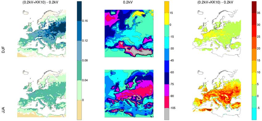
662                                              G. Strandberg et al.: Sensitivity to changes in anthropogenic deforestation

from the KK10 scenario (V + KK10). The climate model re-          ied on a global scale (e.g. Brovkin et al., 2006; Pitman et al.,
sults show that the simulated effects of deforestation depend     2009; Pongratz et al., 2009b, 2010; de Noblet-Ducoudré et
on both local/regional climate and vegetation characteristics.    al., 2012; Christidis et al., 2013).
At ∼ 6 k BP the extent of simulated deforestation in Europe          Global climate models (GCMs) are run on coarse spatial
is generally small, but there are areas where deforestation       resolutions; therefore, they can only reproduce large-scale
is large enough to produce significant differences in sum-        climate features. Regional climate models (RCMs) preserve
mer temperatures of 0.5–1 ◦ C. At ∼ 0.2 k BP, extensive de-       the large-scale climate features, but the higher spatial reso-
forestation, particularly according to the KK10 model, leads      lution in RCMs provides a better representation of the land–
to significant temperature differences in large parts of Eu-      sea distribution and topography, which in turn allows a more
rope in both winter and summer. In winter, deforestation          detailed description of the regional climate (Rummukainen,
leads to lower temperatures because of the differences in         2010). This also applies to vegetation modelling. Only a de-
albedo between forested and unforested areas, particularly        tailed description of vegetation can account for biogeophysi-
in the snow-covered regions. In summer, deforestation leads       cal effects on climate at the regional scale (Wramneby et al.,
to higher temperatures in central and eastern Europe because      2010). Since we expect vegetation change to affect climate
evapotranspiration from unforested areas is lower than from       at the local/regional spatial scale, a high spatial resolution in
forests. Summer evaporation is already limited in the south-      the climate model is critical when evaluating model results
ernmost parts of Europe under potential vegetation condi-         by comparison with observations and/or proxies that repre-
tions and, therefore, cannot become much lower. Accord-           sent local to regional environment conditions. To date there
ingly, the albedo effect dominates in southern Europe also in     are no previous RCM-based studies of the feedback on cli-
summer, which implies that deforestation causes a decrease        mate from historical changes in land use/anthropogenic land
in temperatures. Differences in summer temperature due to         cover.
deforestation range from −1 ◦ C in south-western Europe to           The present study investigates the direct effect on cli-
+1 ◦ C in eastern Europe. The choice of anthropogenic land-       mate from human-induced vegetation changes in Europe at
cover scenario has a significant influence on the simulated       the regional spatial scale. We do not study the indirect ef-
climate, but uncertainties in palaeoclimate proxy data for the    fects from changing atmospheric CO2 concentration. This
two time periods do not allow for a definitive discrimination     study is part of the LANDCLIM (LAND cover–CLIMate in-
among climate model results.                                      teractions in NW Europe during the Holocene) project that
                                                                  aims to assess the possible effects on the climate of two
                                                                  historical processes (compared with a baseline of present-
                                                                  day land cover): (i) climate-driven changes in vegetation and
1     Introduction                                                (ii) human-induced changes in land cover (Gaillard et al.,
                                                                  2010). Specifically, this study asks (i) whether historical land
Humans potentially had an influence on the climate system         use influences the regional climate, (ii) how much the RCM-
through deforestation and early agriculture already long be-      simulated climate differs depending on the scenario of past
fore we started to emit CO2 from fossil fuel combustion           anthropogenic land cover used, (iii) which processes are im-
(Ruddiman, 2003). Deforestation affects the climate at many       portant for climate–vegetation interaction, and (iv) to what
scales, from microclimate to global climate (e.g. Bala et al.,    extent palaeoclimate proxy data are effective at evaluating
2007). The effect on the global climate is conveyed by the        RCM-based simulation results.
increased amounts of CO2 in the atmosphere from deforesta-           We focus on two contrasting time periods in terms of
tion, and by the regional and local changes of land-surface       climate and anthropogenic land cover change: the Mid-
properties (e.g. Forster et al., 2007). Such changes have a       Holocene warm period (∼ 6 k BP) and the Little Ice Age
direct effect on the regional climate, including changes in       (∼ 0.2 k BP = ∼ AD 1750). The Mid-Holocene was charac-
albedo and energy fluxes between the land surface and the         terised by a relatively warm climate and low human impact
atmosphere (e.g. Pielke et al., 2011). Since forests generally    on vegetation/land cover, while the Little Ice Age was cool
have a lower reflectivity than unforested areas, the albedo ef-   and anthropogenic land use was extensive. The 6 k time-
fect from deforestation would lead to lower regional temper-      window has the advantage of being widely used in model-
ature. Reduced vegetation cover also means reduced evap-          data comparison studies of global climate models (e.g. Har-
otranspiration that leads to higher air temperature, but the      rison et al., 1998; Masson et al., 1999; Kohfeld and Harri-
amplitude of the evapotranspiration changes depend on local       son, 2000; see the Palaeoclimate Modelling Intercomparison
conditions, such as soil moisture availability (Ban-Weiss et      Project (PMIP) activities: http://pmip.lsce.ipsl.fr/), which al-
al., 2011; de Noblet-Ducoudré et al., 2012). The effects of in-   lows us to set our results in a wider perspective. We use a
creased atmospheric CO2 resulting from changing vegetation        dynamic vegetation model, LPJ-GUESS (Smith et al., 2001),
and land use over the last 8000 yr have been previously dis-      to simulate past climate-driven potential natural vegetation
cussed (e.g. Ruddiman, 2003; Pongratz et al., 2009a). The di-     and two alternative scenarios of anthropogenic land-cover
rect effects of past vegetation change have mostly been stud-     change (ALCC): HYDE3.1 (History Database of the Global

Clim. Past, 10, 661–680, 2014                                                                 www.clim-past.net/10/661/2014/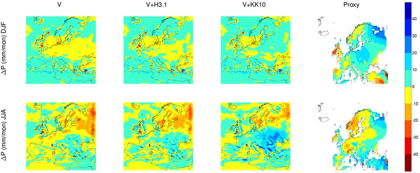
G. Strandberg et al.: Sensitivity to changes in anthropogenic deforestation                                                          663

Table 1. Summary of forcing conditions in the RCA3 simulations; see text for details. The amount of greenhouse gases and irradiance varies
from year to year, and the table shows average values.

                                                                                                            Total solar
                                                                                 CO2      CH4      N2 O     irradiance
                    Name                Period       Vegetation     Land use    (ppm)    (ppb)    (ppb)      (W m−2 )
                    6 kV                                              None
                    6kV + H3.1          6 k BP     Potential 6 k   HYDE3.1        265      572      260          1364
                    6kV + KK10                                       KK10
                    0.2 kV                                            None
                    0.2kV + H3.1      0.2 k BP   Potential 0.2 k   HYDE3.1        277      710      277          1363
                    0.2kV + KK10                                     KK10

Environment; Klein Goldewijk et al., 2011) and KK10 (Ka-               used to drive the vegetation model LPJ-GUESS to simu-
plan et al., 2009). These scenarios of past human-induced              late potential vegetation. For each time period, three 50 yr
vegetation are widely used in climate modelling of the past,           long RCA3 simulations are then performed with three alter-
but they exhibit large differences for key periods of the              native land-cover/vegetation descriptions: (i) potential veg-
Holocene (Gaillard et al., 2010; Boyle et al., 2011). These            etation without human impact (V), (ii) V with the addi-
discrepancies are due to differences in the modelling ap-              tion of the HYDE3.1 estimate of anthropogenic deforestation
proach. While previous studies demonstrated the large influ-           (V + H3.1), and (iii) V with the addition of the KK10 esti-
ence of the choice of ALCC scenario on modelled changes                mate of anthropogenic deforestation (V + KK10). The itera-
in terrestrial carbon storage over the Holocene (Kaplan et al.,        tive modelling approach of RCM and DVM, RCA3 → LPJ-
2009), little work has been done to assess the importance of           GUESS → RCA3, has been shown to be a reasonable ap-
the ALCC scenario used with respect to the biogeophysical              proach where both simulated climate and vegetation are in
feedback to climate. We therefore use both HYDE and KK10               general agreement with available reconstructions, which are
in our model simulations of regional climate.                          few and uncertain (Kjellström et al., 2010; Strandberg et al.,
   In order to evaluate the RCM-simulated results, we use cli-         2011). The simulations are summarised in Table 1. If not
mate proxy records based on (i) the LANDCLIM database of               stated otherwise, “model simulation” stands for a simulation
point data, i.e. representing either local or regional climate         with RCA3 forced with data from the other models described
conditions based on non-pollen proxies (e.g. tree-ring data,           below.
chironomid records from lake sediments, stalagmite δ 18 O
records, etc.; Nielsen et al., 2014) to avoid any circular rea-        2.1.1   The general circulation model ECHO-G
soning (where the same vegetation would be used both to
force and evaluate the model simulations), and (ii) an attempt
                                                                       ECHO-G has been used and evaluated earlier in palaeocli-
at spatially explicit descriptions of past climate characteris-
                                                                       matic studies (Zorita et al., 2005; Kaspar et al., 2007) and
tics based on pollen data (Mauri et al., 2013).
                                                                       has provided climate simulations in regional studies (e.g.
                                                                       Gómez-Navarro et al., 2011, 2012; Schimanke et al., 2012).
2     Material and methods                                             Here, we use results from the transient Oetzi2 run cover-
                                                                       ing the period 7000 BP to present (Wagner et al., 2007). In
2.1    The models                                                      Oetzi2, ECHO-G is run with a horizontal resolution of T30
                                                                       (approximately 3.75◦ × 3.75◦ ) and 19 levels in the atmo-
The main tool used in this study to produce high spatial reso-         sphere, and a spatial resolution of approximately 2.8◦ × 2.8◦
lution climate simulations is the Rossby Centre regional cli-          and 20 levels in the oceans. The simulation was initialised
mate model RCA3 (Samuelsson et al., 2011). Here, we de-                at the end of a 500 yr spin-down control (quasi-equilibrium)
scribe RCA3 and the models that provide the boundary con-              run with constant forcing (orbital, solar and greenhouse gas)
ditions for the RCA3 runs. These models include the global             for 7 ka BP.
climate model ECHO-G (Legutke and Voss, 1999), the dy-                    The external forcings used in the global simulation with
namic vegetation model (DVM) LPJ-GUESS (Smith et al.,                  ECHO-G are variations in Total Solar Irradiance (TSI),
2001), and the ALCC scenarios HYDE3.1 and KK10.                        changes in atmospheric concentrations of greenhouse gases
   For each time period RCA3 uses lateral boundary con-                (GHGs), and changes in the Earth’s orbit. The TSI changes
ditions, sea-surface temperature and sea-ice conditions                were derived from the concentration of the cosmogenic iso-
from ECHO-G and in the first run modern-day vegetation                 tope 10 Be in polar ice cores, and translated to TSI by scaling
(Samuelsson et al., 2011). The simulated climate is then               production estimates of δ 14 C (cf. Solanki et al., 2004) such

www.clim-past.net/10/661/2014/                                                                            Clim. Past, 10, 661–680, 2014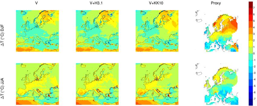
664                                               G. Strandberg et al.: Sensitivity to changes in anthropogenic deforestation

that the difference between present-day and Maunder Mini-
mum solar activity is 0.3 %. Past greenhouse gas concentra-
tions were also estimated from air bubbles trapped in polar
ice cores (Flückiger et al., 2002). Finally, the changes in the
orbital parameters obliquity, eccentricity and position of the
perihelion can be accurately calculated for the last few mil-
lion years (Berger and Loutre, 1991).
   The vegetation in the global model is set to present-day
conditions for both simulations. Because the ECHO-G model
has a very coarse resolution, vegetation changes in Europe
are assumed not to have an overwhelming effect on the large
scale atmospheric and oceanic circulation upstream, such as
the North Atlantic Oscillation (NAO) and North Atlantic sea-
surface temperatures.

2.1.2   The Rossby Centre regional atmospheric climate
        model RCA3
                                                                    Fig. 1. Difference in land–sea distribution between 6 and 0.2 k BP;
RCA3 is used to downscale results from ECHO-G to higher
                                                                    grid boxes with a difference of more than 50 % are shaded. The
resolution. RCA3 and its predecessors RCA1 and RCA2
                                                                    three regions used for analysis in Fig. 11 are marked as red squares;
have been extensively used and evaluated in studies of              Iberian Peninsula (IB), western Europe (WE), eastern Europe (EE).
present and future climate (e.g. Rummukainen et al., 2001;          The blue boxes represent the regions northern Europe and southern
Räisänen et al., 2004; Kjellström et al., 2011; Nikulin et al.,     Europe described in Sect. 4.2.
2011). Also, RCA3 has been used in palaeoclimatological
applications for downscaling global model results for the last
millennium (Graham et al., 2009; Schimanke et al., 2012),           tical levels and a time step of 30 min. Data for initialising
parts of the Marine Isotope Stage 3 (Kjellström et al., 2010),      RCA3 are taken from ECHO-G. After that, every 12 h, RCA3
and for the Last Glacial Maximum (Strandberg et al., 2011).         reads surface pressure, humidity, temperature and wind from
   In RCA3, the present-day land–sea distribution and sur-          ECHO-G along the lateral boundaries of the model domain,
face geopotential is used for 0.2 k. The land–sea distribution      and sea-surface temperature and sea-ice extent within the
for 6 k is taken from the ICE-5G database (Peltier, 2004). The      model domain. All RCA3 simulations have been run for 50 yr
difference in orography between the two periods is caused by        with 1 yr spin-up time (simulated years are 3909–3861 BC
the changed coastline and the less detailed coastline in ICE-       for 6 k and AD 1701–1750 for 0.2 k), after which the effect
5G. Land and sea grid cells are therefore not exactly the same      of the initial conditions of atmosphere/land surface system
in the two periods (Fig. 1).                                        are assumed to have faded (Giorgi and Mearns, 1999).
   ECHO-G and RCA3 use the same solar irradiance. The                  For each simulation of a 50 yr period we calculate the av-
concentrations of atmospheric GHG in RCA3 are repre-                erage of the nominal seasons winter (December, January and
sented as CO2 -equivalents, whereas in ECHO-G CO2 and               February; henceforth DJF) and summer (June, July and Au-
CH4 are explicitly described. GHGs and solar irradiance             gust; henceforth JJA). In addition, the diurnal cycle is anal-
change from year to year and are read annually by the mod-          ysed for some regions.
els. Table 1 summarises the forcing from GHGs and insola-              The statistical significance for the difference between
tion averaged over the two periods.                                 the simulations is determined by a bootstrapping technique
   For snow in unforested areas, RCA3 has a prognostic              (Efron, 1979). 500 bootstrap samples are used to estimate the
albedo that varies between 0.6–0.85; the albedo decreases as        inter-annual variability of seasonal and annual means of tem-
snow ages. For snow-covered land areas in forest regions the        perature, precipitation, latent heat flux and albedo for each
albedo is set constant to 0.2. The snow-free albedo is set to       simulation. The difference between two simulations is com-
0.28 and 0.15 for unforested and forested areas, respectively.      pared with the estimated distribution of a parameter (e.g.
Leaf Area Index (LAI) is calculated as a function of the soil       temperature) to see if the difference is statistically signifi-
temperature with a lower limit set to 0.4, and upper limits to      cant. We choose the 95 % level for significance.
2.3 (unforested) and 4.0 (deciduous forest). If deep soil mois-
ture reaches the wilting point the LAI is set to its lower limit.   2.1.3   The dynamic vegetation model LPJ-GUESS
LAI in coniferous forests is set constant to 4.0 regardless of
soil moisture (Samuelsson et al., 2011).                            LPJ-GUESS (Smith et al., 2001; Hickler et al., 2004, 2012)
   RCA3 is run on a horizontal grid spacing of 0.44◦ (corre-        is used to simulate potential natural vegetation patterns con-
sponding to approximately 50 km) over Europe with 24 ver-           sistent with the simulated climate in Europe during the two

Clim. Past, 10, 661–680, 2014                                                                     www.clim-past.net/10/661/2014/
G. Strandberg et al.: Sensitivity to changes in anthropogenic deforestation                                                     665

selected time windows. The model has been previously used           land-use categories are summed up to represent the total frac-
to simulate past vegetation (Miller et al., 2008; Garreta et al.,   tion of anthropogenic deforestation. Upscaled (averaged to a
2010; Kjellström et al., 2010; Strandberg et al., 2011) and         0.5◦ resolution) versions of both data sets for the two selected
to assess the effects of land use on the global carbon cycle        time windows are used as input in the RCM runs (Fig. 2).
(Olofsson and Hickler, 2008; Olofsson, 2013).                          While proxy-based quantitative information on anthro-
   LPJ-GUESS is a process-based dynamic ecosystem model             pogenic land use before the 20th century is rare, KK10
designed for application at regional to global spatial scales. It   and HYDE3.1 have been evaluated in western Europe north
incorporates representations of terrestrial vegetation dynam-       of the Alps (the LANDCLIM project study region) using
ics based on interactions between individual trees and shrubs       pollen-based quantitative reconstructions of vegetation cover
and a herbaceous understory at neighbourhood (patch) scale          based on the “Regional Estimates of VEgetation Abundance
(Hickler et al., 2004). It accounts for the effect of stochasti-    from Large Sites” (REVEALS) model (Sugita, 2007). RE-
cally recurring disturbances for heterogeneity among patches        VEALS is a mechanistic model of pollen dispersal that
in terms of accrued biomass, vegetation composition and             can reduce biases caused by inter-taxonomic differences in
structure at the landscape scale. The simulated vegetation is       pollen productivity and dispersal/deposition characteristics
represented by Plant Functional Types (PFTs; Table 2) dis-          properties. The comparison of KK10 and HYDE3.1 with the
criminated in terms of bioclimatic limits to survival and re-       REVEALS-model estimates of open land for five time win-
production, leaf phenology, allometry, life-history strategy        dows of the Holocene – 6000, 3000, 600, 200 cal yr BP and
and aspects of physiology governing carbon balance and              recent past (LANDCLIM vegetation data set; Gaillard, 2013;
canopy gas-exchange. Differences between PFTs in combi-             Trondman et al., 2013) – shows that the KK10 scenarios tend
nation with the present structure of the vegetation in each         to be more similar to the REVEALS-based reconstruction
patch govern the partitioning of light and soil water among         of vegetation cover than the HYDE3.1 scenarios (Kaplan et
individuals as well as regeneration and mortality, affecting        al., 2014). The REVEALS estimates of open land for the
competition among PFTs and age/size classes of plants.              two time windows used in this study are shown in Fig. 2
   Inputs to the model are temperature (◦ C), precipita-            for comparison.
tion (mm), net downward short-wave radiation at surface
(W m−2 ) and wet day frequency (days), all in monthly               2.2   Alternative land-cover descriptions used in the
timesteps provided by RCA3 at a 0.44◦ spatial resolution                  RCA3 runs
over Europe and annual atmospheric CO2 concentration for
the 6 and 0.2 k time windows. The static, present-day soil          Potential natural land cover (hereafter referred to as V) for
texture data described in Sitch et al. (2003) were used dur-        6 and 0.2 k is simulated using LPJ-GUESS (forced with re-
ing all simulations. The PFT determination was based on the         sults from RCA3). The resulting LAI per PFT and per grid
European dominant species version described by Hickler et           cell is averaged over the modelling period for both time win-
al. (2012) (Table 2).                                               dows and then converted to foliage projective cover (FPC).
                                                                    The FPC is defined, applying the Lambert–Beer law (Monsi
2.1.4   The anthropogenic land cover change                         and Saeki, 1953), as the area of ground covered by foliage
        scenarios KK10 and HYDE3.1                                  directly above it (Sitch et al., 2003):

                                                                    FPC(PFT) = 1.0 − exp(−k ∗ (LAI(PFT))),
The historical ALCC scenarios most often used in earth sys-
tem modelling are HYDE3.1 (Klein Goldewijk et al., 2011),           where k is the extinction coefficient (0.5).
KK10 (Kaplan et al., 2009) and the scenarios of Pongratz               The calculated species-specific FPC-values were summed
et al. (2009b). We have chosen HYDE3.1 and KK10 for                 up to three RCA3-specific PFTs (Table 2) per grid cell. The
this study because they represent the two extremes of esti-         fraction of non-vegetated land is calculated by subtracting
mated anthropogenic impact at the two selected time win-            the sum of all the PFT-values per grid cell from one.
dows. These ALCC models use similar estimates of past                  In order to obtain a description of the land cover including
human population density, but differ in their estimates of          information on both natural and human-induced vegetation
land requirement per capita and the assessment of the effect        the LPJ-GUESS simulation results (V) are combined with
of contrasting technological development between regions.           the two ALCC simulations, KK10 and H3.1. The V + KK10
Therefore, they provide substantially different scenarios of        and V + H3.1 vegetation descriptions are constructed by sub-
the extent of deforestation and land-use intensity (Gaillard et     tracting the ALCC fraction determined by KK10 or H3.1
al., 2010; Boyle et al., 2011; Kaplan et al., 2011).                from one, and thereafter homogeneously rescaling the PFT
   KK10 represents the total amount of the land fraction used       values provided by V in all grid cells to fit into the remain-
for agrarian activities at a 50 spatial resolution. The HYDE3.1     ing space. The total unforested fraction is then calculated by
(hereafter referred to as H3.1, HYDE, 2011) land-use data set       summing up the ALCC KK10 or H3.1 with the LPJ-GUESS
includes information on the fraction of cropland, grassland         simulated PFT Grass fractions in each grid cell.
and urban areas, also at a 50 spatial resolution. The different

www.clim-past.net/10/661/2014/                                                                     Clim. Past, 10, 661–680, 2014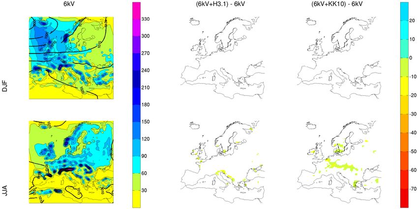
666                                                                G. Strandberg et al.: Sensitivity to changes in anthropogenic deforestation

Table 2. The three plant functional types (PFTs) for regional climate model RCA3; LPJ-GUESS PFTs according to Hickler et al. (2012) and
Wolf et al. (2008); LANDCLIM REVEALS taxa (Mazier et al., 2012); and modern analogue technique (MAT) PFTs adapted from Peyron et
al. (1998).

           RCA3 PFT                      LPJ-GUESS PFT                                  LANDCLIM              REVEALS            MAT PFT
                                                                                        taxa*
                                         Picea_abies                                    Picea                                    Boreal evergreen/ cool-temperate
                                                                                                                                 conifer
                                         Abies_alba                                     Abies
           Coniferous
           tree                          Pinus_sylvestris, P. halepensis                Pinus
           canopy
                                         Tall shrub evergreen, Juniperus                Juniperus                                Eurythermic conifer
                                         oxycedrus
                                                                                                                                 Boreal summergreen
                                                                                                                                 Intermediate temperate
                                                                                        Alnus                                    Temperate/boreal
                                                                                                                                 summergreen/arctic-alpine
                                         Betula pendula, B. pubescens                   Betula                                   Boreal summergreen
                                                                                                                                 arctic-alpine
                                         Corylus avellana                               Corylus                                  Cool-temperate summergreen
                                         Carpinus betulus                               Carpinus
                                         Fagus sylvatica                                Fagus
                                         Fraxinus excelsior                             Fraxinus                                 Temperate summergreen
                                         Mediterranean rain green shrub

           Broad-leaved                  Populus tremula                                                                         Temperate/boreal summergreen
           tree                          Quercus coccifera, Q. ilex                     Quercus                                  Warm-temperate broad-leaved
           canopy                                                                                                                evergreen
                                         Quercus pubescens, Q. robur                                                             Temperate summergreen
                                         Tilia cordata                                  Tilia                                    Cool-temperate summergreen
                                         Ulmus glabra                                   Ulmus
                                         Tall shrub summergreen                         Salix                                    Temperate/boreal
                                                                                                                                 summergreen/arctic-alpine
                                                                                                                                 Warm-temperate summergreen
                                                                                                                                 Cool-tremperate broad-leaved
                                                                                                                                 evergreen
                                                                                                                                 Warm-temperate
                                                                                                                                 Warm-temperate sclerophyll
                                                                                                                                 trees/shrub
           Unforested                    C3 Grass                                       Cereals (Secale excluded)                Non arboreal
                                                                                        /Cerealia-t, Secale, Cal-
                                                                                        luna, Artemisia, Cyper-
                                                                                        aceae, Filipendula, Plan-
                                                                                        tago lanceolata, P. mon-
                                                                                        tana, P. media, Poaceae,
                                                                                        Rumex p.p. (mainly R.
                                                                                        acetosa R. acetosella)/R.
                                                                                        acetosa-t
         * These taxa have specific pollen-morphological types. When the latter correspond to a botanical taxon, they have the same name; if not, it is indicated by the
         extension “-t”.

Clim. Past, 10, 661–680, 2014                                                                                                          www.clim-past.net/10/661/2014/
G. Strandberg et al.: Sensitivity to changes in anthropogenic deforestation 667
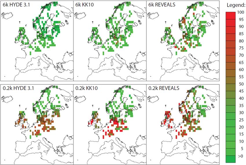
Fig. 2. The anthropogenic land-use scenarios HYDE3.1 (Klein Goldewijk et al., 2011) and KK10 (Kaplan et al., 2009), and the grid-based
(GB) REVEALS reconstructions (Trondman et al., 2013) at 6 and 0.2 k BP and a spatial scale of 1’. The colour coding represents the degree
of human-induced deforestation in % cover (HYDE3.1 and KK10) and the % cover of plants characteristic of grassland (primarily grasses,
sedges, sorrel and a few other herbs) and cultivated land (cereals) as estimated by the REVEALS model using pollen data. Reddish to red
colours represent > 50 % deforestation, and green colours < 50 % deforestation, These maps are not directly comparable as the methods used
in the model scenarios follow a totally different approach, and the REVEALS-based reconstructions represent actual openness, natural and
human-induced (see method section for more details). Nevertheless, these maps show that in several areas of Europe, in particular western
Europe (e.g. Britain, France, Switzerland, Germany), the KK10 scenarios are closer to the pollen-based REVEALS reconstructions than the
HYDE3.1 scenarios in terms of intensity of human land use, given that there was little natural openness at 6 k and most of the openness at
0.2 k was human induced. A more in-depth/sophisticated comparison of these scenarios and the REVEALS reconstructions are discussed in
detail in Kaplan et al. (2014).
The simulated V, V + H3.1 and V + KK10 land-cover de- the pollen data used might bias the climate reconstruction
scriptions are recalculated to 100 % vegetation, omitting the due to significant human-induced changes in vegetation from
non-vegetated fraction and upscaled to a 1◦ spatial resolu- ca. 3 k (e.g. Gaillard, 2013) (see discussion). For the south-
tion. The agreement of the three sets of results is assessed by ern and eastern parts of the study area covered by the RCA3
comparison of the dominant (> 50 %) land cover type (un- simulations but not by the LANDCLIM database, we rely
forested or forested) between the sets. primarily on the non-pollen proxy-based climate reconstruc-
tions presented in Magny and Combourieu Nebout (2013),
2.3 Proxy data of past climate and in particular the synthesis of palaeohydrological changes
and their climatic implications in the central Mediterranean
We use two proxy data sets of past climate for compari- region and its surroundings (Magny et al., 2013). The Mauri
son with the RCA3 climate simulations at 6 and 0.2 k: the et al. (2013) reconstruction in the Mediterranean area is
LANDCLIM database of past climate proxy records, consist- also compared to the pollen-based climate reconstructions in
ing mainly of site specific/point reconstructions of past cli- the Mediterranean region published by Peyron et al. (2013).
mate based on non-pollen proxies (Nielsen et al., 2014); and The latter reconstructions are based on the multi-method ap-
the spatially explicit pollen-based climate reconstruction of proach that uses a combination of pollen-based weighted av-
Mauri et al. (2013). The LANDCLIM project itself is con- eraging, weighted-average partial least-squares regression,
cerned about circular reasoning and avoids using climate modern analogue technique (MAT), and non-metric multi-
reconstructions based on pollen records because the RE- dimensional scaling/generalized additive model methods.
VEALS reconstructions of vegetation cover are also based The LANDCLIM database of past climate records in-
on pollen records (see below). Nevertheless, in this study, we cludes data sets of palaeoecological proxies, data from writ-
chose to also use a pollen-based reconstruction of climate for ten archives and instrumental measurements from 245 sites
Europe because it is the only spatially explicit description of in western Europe north of the Alps for the two time
past climate existing to date, keeping in mind, however, that
www.clim-past.net/10/661/2014/ Clim. Past, 10, 661–680, 2014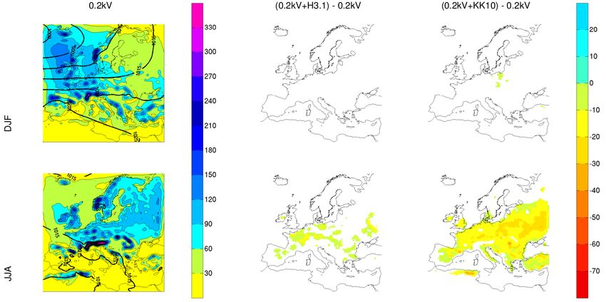
668                                               G. Strandberg et al.: Sensitivity to changes in anthropogenic deforestation

windows 6 k (5700–6200 BP) and 0.2 k (AD 1700–1800) as              ous trees, while western and lowland Europe is dominated
well as for the time after AD 1960. Climate reconstruc-             by broad-leaved trees. The average HYDE3.1 anthropogenic
tions based on proxies of vegetation (plant macrofossils and        land cover/deforestation (H3.1) at 6 k is generally < 1 %;
pollen) are excluded from the database to avoid circular rea-       values > 5 % are restricted to some areas of southern Eu-
soning. The selected reconstructions are dated with mul-            rope (Fig. 3). Therefore, the V + H3.1 land cover descrip-
tiple radiocarbon dates of terrestrial plant material, varve        tion does not differ markedly from V. The KK10 estimates
counts, dendrochronology, TIMS (thermal ionisation mass             of deforestation are higher (> 4 % in average) and reach val-
spectrometry)-dated speleothems or historical records. To           ues > 50 % in southern Europe and restricted areas of south-
compare our model-simulated climate results with empirical          ern Scandinavia, Belgium and the northern Alps. However,
climate reconstructions, we used primarily the proxies based        the additional unforested land predicted by HYDE3.1 and
on diatoms, tree rings and chironomids for summer tempera-          KK10 is negligible in comparison to the potential unforested
tures (July T ), and proxies based on lake-level changes, varve     land simulated by LPJ-GUESS, which explains why the V,
thickness in lake sediments, and 13 C and 18 O in carbonates        V + H3.1 and V + KK10 land cover descriptions do not dif-
for relative changes in yearly precipitation minus evaporation      fer significantly from each other at 6 k.
(P -E).                                                                The V land-cover description at 0.2 k shows little differ-
   The climate reconstruction of Mauri et al. (2013) largely        ence compared to V at 6 k (Fig. 3). The largest differences
follows the modern analogue technique (MAT) approach de-            are found in Scandinavia where areas with less than 50 % of
scribed in Davis et al. (2003), but it is based on much im-         forest cover are much larger than they are at 6 k. The average
proved pollen data sets. The modern surface sample data set         H3.1 estimates of deforestation are ca. 10 %, but reach values
was compiled from the European Modern Pollen Database               > 50 % in southern Europe. The KK10 estimates of anthro-
(Davis et al., 2013) and represents a substantial improvement       pogenic deforestation are > 40 % on average and the high-
compared to that used in Davis et al. (2003), with an increase      est values (> 95 %) are found in southern Europe. Owing
in the number of samples by ∼ 80 % (total of 4287 sites). The       to the high KK10 estimates in most of western, central and
fossil data set includes 48 % more sites (total of 756 sites)       southern Europe, the forest cover is considerably reduced in
compared with Davis et al. (2003), with this improvement            V + KK10 in comparison to V + H3.1 and particularly to V.
in data coverage spread throughout Europe. The MAT ap-
proach calculates a pollen–climate transfer function to recon-      3.2   Simulated climate
struct palaeoclimate from fossil pollen data, where the fossil
and modern pollen samples are matched using pollen assem-           The overall features of the simulated 6 and 0.2 kV regional
blages grouped into PFTs (Table 2). The use of PFT groups           climate are comparable. Winter (DJF) mean temperatures
allows a wider range of taxa to be included in the analysis         range from −15 ◦ C in northern Europe to 10 ◦ C over the
without over-tuning the transfer function, and allows taxa to       Iberian Peninsula (Figs. 4 and 5, upper left panels). In sum-
be included that may not be present in the modern pollen            mer (JJA), the highest temperatures (ca. 20 ◦ C) occur in
calibration data set. Since PFT groups are largely defined ac-      the Mediterranean region, while summer mean temperatures
cording to their climatic affinities (Prentice et al., 1996), the   do not reach more than ca. 10 ◦ C in northern Scandinavia
approach also reduces the sensitivity of the transfer function      (Figs. 4 and 5, lower left panel). Summer temperatures at
to non-climatic influences, such as human impact on vege-           6 k are ca. 0–2 ◦ C warmer than at 0.2 k in most of Europe
tation, disease, ecological competition or succession, or soil      (Fig. 6). In winter, northern Europe is 1–2 ◦ C warmer at 6 k
processes. Approximate standard errors for the reconstruc-          than at 0.2 k, while large parts of central Europe are ca. 0.5 ◦ C
tion were calculated following Bartlein et al. (2010) by as-        colder.
similating samples at the interpolated spatial grid resolution,        The largest precipitation amounts in winter (100–
together with the standard error from the interpolation itself.     150 mm month−1 ) fall in the western parts and mountain
                                                                    ranges of the study area, while the smallest amounts (30–
                                                                    60 mm month−1 ) are found in the eastern regions (Figs. 7
3     Results                                                       and 8, top rows). In summer, most precipitation (60–
                                                                    100 mm month−1 ) falls over the land areas of the northern
3.1    LPJ-GUESS simulated vegetation                               half of Europe, and the least around the Mediterranean (0–
                                                                    50 mm month−1 ) (Figs. 7 and 8, bottom rows). The only sig-
The simulated potential vegetation (V) at 6 k is characterised      nificant differences in precipitation are seen in summer in
by a forest cover of > 90 % in most of Europe (Fig. 3). The         parts of eastern and central Europe where 6 kV is drier than
areas with less than 50 % of forest cover (central Alps, Scan-      0.2 kV by 10–20 mm month−1 (Fig. 9).
dinavian mountains, northern Scandinavia and Iceland) are              The difference between the simulated V climate and
typically related to high elevations and/or latitudes. The sim-     the V + H3.1 or V + KK10 climate at 6 k is generally not
ulated forest composition of northern and eastern Europe and        statistically significant, but the V + KK10 climate exhibits
elevated areas of central Europe is dominated by conifer-           a few hotspots (southern Scandinavia, Belgium, north of

Clim. Past, 10, 661–680, 2014                                                                    www.clim-past.net/10/661/2014/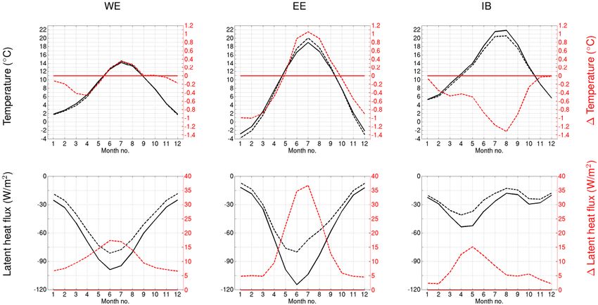
G. Strandberg et al.: Sensitivity to changes in anthropogenic deforestation                                                              669

Fig. 3. Proportion of the LPJ-GUESS simulated potential natural vegetation cover (V) represented by fraction of forest (columns 1 and 3) and
three RCA3 PFTs (i.e. broad-leaved trees, needle-leaved trees and unforested) (columns 2 and 4) at 6 k BP (columns 1 and 2) and 0.2 k BP
(columns 3 and 4). The simulation is forced by the initial RCA3 model-simulated climate. The simulated vegetation cover (V) is post-
processed by overlaying the anthropogenic deforestation scenarios from the HYDE 3.1 database (Klein Goldewijk et al., 2010) (V + H3.1)
and the KK10 scenarios of Kaplan et al. (2009) (V + K). The colour scales indicates the fractions of forest and the PFTs within each grid box.

the Alps) with summer temperatures 0.5–1 ◦ C warmer than                 southern Scandinavia in the V + KK10 simulation, in some
the V simulation (Fig. 4). Winter precipitation hardly dif-              regions with as much as a 1–1.5 ◦ C difference between the
fers between the 6 k V, V + H3.1 and V + KK10 simulations,               V + KK10 and V simulations. However, the winter tempera-
whereas small but statistically significant differences in sum-          ture differences between all simulations are statistically sig-
mer precipitation (not more than −10 mm month−1 ) between                nificant only in parts of eastern Europe. Summer (JJA) tem-
the 6 k V + KK10 simulation and the other two 6 k simula-                peratures at 0.2 k are also lower (Fig. 5, bottom row), but
tions are found mostly in central Europe (Fig. 7). The un-               only in the Mediterranean region, again most pronounced in
changed precipitation pattern during winter in between the               the V + KK10 simulation. Conversely, higher summer tem-
different RCA3 simulations might be due to the large influ-              peratures by up to 1 ◦ C in parts of eastern Europe are a par-
ence of the large-scale atmospheric circulation during winter,           ticular feature in the V + KK10 simulation at 0.2 k. Summer
inheriting the information from ECHO-G into RCA3. During                 precipitation is lower by 0–20 mm month−1 in scattered parts
summer this effect is much less, and more regional-to-local              of central and southern Europe in the V + H3.1 simulation at
scale effects influence precipitation patterns.                          0.2 k, while it is lower in all regions where the simulated for-
   At 0.2 k, deforestation (V + H3.1 and V + KK10) leads to              est fraction is reduced by more than 50 % in the V + KK10
lower winter (DJF) temperatures than potential vegetation                simulation, with statistically significant differences of −10 to
(V) (Fig. 5, top row). The lower temperatures are confined               −30 mm month−1 in most of Europe (Fig. 8). Differences in
to the Alps and parts of eastern Europe in the V + H3.1 sim-             winter precipitation between the simulations are very small.
ulation, while they are found in all of eastern Europe and

www.clim-past.net/10/661/2014/                                                                            Clim. Past, 10, 661–680, 2014
670                                                 G. Strandberg et al.: Sensitivity to changes in anthropogenic deforestation

Fig. 4. Temperature (◦ C) at 6 k BP for winter (top row) and summer (bottom row). Absolute temperature from run 6 kV (left), difference
6 kV + H3.1–6 kV (middle) and 6 kV + KK10–6 kV (right). In the middle and right panels, grid boxes with a significant temperature difference
at the 95 % level are coloured. Isolines show changes in the remaining regions. The “zero isoline” is excluded.

Fig. 5. Temperature (◦ C) at 0.2 k BP for winter (top row) and summer (bottom row). Absolute temperature from run 0.2 kV (left), difference
0.2 kV + H3.1–0.2 kV (middle) and difference 0.2kV + KK10–0.2kV (right). In the middle and right panels, grid boxes with a significant
temperature difference at the 95 % level are coloured. Isolines show changes in the remaining regions. The “zero isoline” is excluded.

   The difference between the 6 and 0.2 k simulations (6–               south-west Europe (by 1–2 ◦ C higher) than in eastern Eu-
0.2 k) greatly depends on the vegetation description used               rope (by ca. 1 ◦ C). High values of deforestation at 0.2 k yield
in the climate model runs, i.e. V, V + H3.1 or V + KK10                 larger differences in (i) winter temperatures in eastern Eu-
(Figs. 6 and 9). The climate simulations using vegetation               rope (by 1–2 ◦ C higher at 0.2 k than at 6 k), while small or
descriptions with high values of deforestation (V + KK10)               no differences are seen in the rest of Europe (Fig. 6), and
yield larger 6–0.2 k differences in summer temperature in               (ii) summer precipitation in south-east Europe (by around

Clim. Past, 10, 661–680, 2014                                                                         www.clim-past.net/10/661/2014/
G. Strandberg et al.: Sensitivity to changes in anthropogenic deforestation                                                               671

Fig. 6. Difference between RCA3 runs at 6 and 0.2 k BP (6–0.2 k) (columns 1–3) and pollen-based reconstruction (column 4) for temperature
(1T , ◦ C) in winter (DJF, top row) and summer (JJA, bottom row). Note that the map projection differs from the model results and proxy
estimates.

Fig. 7. Precipitation (mm month−1 ) at 6 k BP for winter (top row) and summer (bottom row). Absolute precipitation and pressure from run
6 kV (left), difference 6kV + H3.1–6 kV (middle) and difference 6kV + KK10–6 kV (right). In the left panels isolines indicate pressure (hPa).
In the middle and right panels grid boxes with a significant precipitation difference at the 95 % level are coloured. Isolines show differences
in the remaining regions. The “zero isoline” is excluded.

30 mm month−1 higher at 0.2 than 6 k). In contrast, large de-             3.3   Climate response to land-use changes
forestation at 0.2 k leads to smaller differences in winter pre-
cipitation between 0.2 and 6 k in central Europe (Fig. 9).                The largest differences in seasonal mean temperature and
   The general effect of changes in the extent of deforestation           precipitation between the RCA3 simulations are found at
on the simulated climate is a change in the amplitude in tem-             0.2 k between the V and V + KK10 simulations. In order to
perature and/or precipitation differences between 6 and 0.2 k             assess the processes behind land cover–climate interactions,
rather than a change in the geographical pattern of those dif-            we analyse the annual cycle of temperature and latent heat
ferences.                                                                 flux at 0.2 k for three regions with particularly large defor-
                                                                          estation but different climate responses (see section above):

www.clim-past.net/10/661/2014/                                                                             Clim. Past, 10, 661–680, 2014
672 G. Strandberg et al.: Sensitivity to changes in anthropogenic deforestation Fig. 8. Precipitation (mm month−1 ) at 0.2 k BP for winter (top row) and summer (bottom row). Absolute precipitation and pressure from run 0.2 kV (left), difference 0.2kV + H3.1–0.2 kV (middle) and difference 0.2kV + KK10–0.2 kV (right). In the left panels isolines indicate pressure (hPa). In the middle and right panels grid boxes with a significant precipitation difference at the 95 % level are coloured. Isolines show differences in the remaining regions. The “zero isoline” is excluded. Fig. 9. Difference between RCA3 runs at 6 and 0.2 k BP (6–0.2 k) (columns 1–3) and pollen-based reconstruction (column 4) for precipitation (1P , mm month−1 ) in winter (DJF, top row) and summer (JJA, bottom row). Note that the map projection differs from the model results and the proxy estimates. western Europe (WE), eastern Europe (EE) and the Iberian forested areas are more readily covered by snow. Moreover, Peninsula (IB). For each region, 3 × 3 grid boxes are selected the effect increases in late winter/spring because of more in- (Fig. 1). coming sunlight. Hence, deforestation leads to larger differ- In winter, lower temperatures due to deforestation are best ences in winter temperature in the north/east, where the snow explained by the albedo effect. The albedo is highest in the season is longer, than in the west/south. V + KK10 simulation since low herb vegetation has a higher When vegetation starts to be active in spring, the albedo ef- albedo than forests (Fig. 10, left column). The difference fect is counteracted by differences in latent heat flux. Gener- in albedo is even higher during the snow season, since un- ally, the larger biomass of forests compared to low vegetation Clim. Past, 10, 661–680, 2014 www.clim-past.net/10/661/2014/
G. Strandberg et al.: Sensitivity to changes in anthropogenic deforestation                                                             673

Fig. 10. Albedo difference, 0.2kV + KK10–0.2 kV (left), absolute latent heat flux (W m−2 ) from run 0.2 kV (middle), and difference in latent
heat flux 0.2kV + KK10–0.2 kV (right) for winter (top) and summer (bottom). In the left and right panels, grid boxes with a significant
difference at the 95 % level are coloured. Isolines show differences in the remaining regions. The “zero isoline” is excluded.

Fig. 11. Annual cycles of temperature (◦ C, top row) and latent heat flux (W m−2 , bottom row) for locations in western Europe (WE),
eastern Europe (EE) and Iberian Peninsula (IB). Black lines show absolute values and red lines show anomalies relative to 0.2 kV. Full black
line: 0.2 kV; dashed black line: 0.2kV + KK10; full red line: 0.2 kV–0.2 kV (i.e. zero difference); dashed red line: 0.2kV + KK10–0.2 kV.
Definitions of WE, EE and IB are found in Fig. 1.

leads to more evapotranspiration and, consequently, lower                ence between the two simulations in summer for WE. WE
temperatures in forested than in deforested regions (Fig. 10,            is also much influenced by the large-scale weather systems
centre and right columns). The differences between the two               from the Atlantic, which makes changes in the regional sur-
simulations in latent heat flux start earlier in the year in WE          face properties less important than in EE. The latent heat flux
compared to EE (Fig. 11, bottom row). Moreover, latent heat              in IB is strongest already in spring. When soils are dry in
flux is weaker in summer and the difference between the                  summer, the latent heat flux is weak and, therefore, the dif-
V + KK10 and V simulations is smaller in WE than in EE,                  ference between the V + KK10 and V simulations is small.
which explains the relatively moderate temperature differ-

www.clim-past.net/10/661/2014/                                                                            Clim. Past, 10, 661–680, 2014
674                                              G. Strandberg et al.: Sensitivity to changes in anthropogenic deforestation

In that case, the change in albedo dominates over the change       Magny, 2007). The fire records published by Vannière et
in latent heat flux, leading to lower summer temperatures.         al. (2011) indicate the same contrasting pattern between the
   Differences in precipitation also correlate with differences    north- and the south-western Mediterranean for the Mid-
in latent heat flux (Figs. 8 and 10). Since differences in pre-    Holocene (including 6 k), with dry summers in the north
cipitation are caused primarily by a change in convective pre-     and humid summers in the south. The evidence presented in
cipitation (not shown), it suggests that convective precipita-     Magny et al. (2013) suggests that, in response to centennial-
tion also changes as a result of deforestation. This would ex-     scale cooling events, drier climatic conditions developed in
plain that 0.2 k is drier in EE than 6 k in the V + KK10 sim-      the south-central Mediterranean, while wetter conditions pre-
ulations. Observations in the tropics have indeed shown that       vailed in the north-central Mediterranean. In general, the cen-
regional deforestation decreases precipitation (Spracklen et       tennial phases of higher lake-level conditions in west-central
al., 2012).                                                        Europe were shown to coincide with cooling events in the
                                                                   North Atlantic area (Bond et al., 2001; e.g. Magny, 2004,
                                                                   2007) and decreases in solar activity before 7 k, and with a
4     Discussion                                                   possible combination of NAO-type circulation and solar forc-
                                                                   ing since ca. 7 k onwards.
4.1    Comparison of the RCA3-simulated regional                      The 6–0.2 k difference in the simulated climate is gener-
       climate with palaeoclimate reconstructions                  ally small for all simulations (V, V + H3.1 and V + KK10)
                                                                   compared to the 6–0.2 k differences in the pollen-based cli-
Studies of diatoms (Korhola et al., 2000; Rosén et al., 2001;      mate reconstructions (PB reconstructions). Moreover, the
Bigler et al., 2006), tree rings (Grudd, 2002; Helama et al.,      geographical/spatial patterns of these 6–0.2 k differences
2002) and chironomids (Rosén et al., 2001; Bigler et al.,          show discrepancies between simulations and reconstructions
2003; Hammarlund et al., 2004; Laroque and Hall, 2004;             (Fig. 6). The difference in summer temperatures ranges from
Velle et al., 2005) indicate a 6–0.2 k difference in summer        ca. +1 ◦ C in Scandinavia to ca. −2 ◦ C in southern Europe
temperature of 0.5–2 ◦ C in Scandinavia, which agrees with         in the PB reconstructions, while it is ca. +2–3 ◦ C in southern
our simulations. Evidence from the presence of Mediter-            and central Europe and ca. +1 ◦ C in northern and eastern Eu-
ranean ostracods in the coastal waters of Denmark sug-             rope in the RCA3 simulations. The difference in winter tem-
gests that winter temperature at 6 k were up to 4–5 ◦ C above      peratures in the PB reconstructions ranges from ca. −3 ◦ C in
present (Vork and Thomsen, 1996). Proxy records of rela-           southern Europe and ca. +3 ◦ C in northern Europe, while the
tive precipitation indicate a drier climate at 6 k than at 0.2 k   RCA3 simulations show a different pattern, with differences
in Scandinavia (Digerfeldt, 1988; Ikonen, 1993; Snowball           ranging from +2–3 ◦ C in Scandinavia to around 0 ◦ C in cen-
and Sandgren, 1996; Hammarlund et al., 2003; Borgmark,             tral Europe and ca. +1 ◦ C in southern Europe. The difference
2005; Olsen et al., 2010), northern Germany (Niggeman et           in insolation in summer between 6 and 0.2 k is positive in all
al., 2003) and the UK (Hughes et al., 2000), while there is no     of Europe, but the difference is larger in northern Europe (see
detectable difference in the Alps (Magny, 2004). Our simu-         Fig. 2 in Wagner et al., 2007). When considering astronom-
lations show similar general features (Figs. 6 and 9). Unfor-      ical forcing alone, we would expect 6 k to be warmer than
tunately, quantitative proxy-based temperature estimates are       0.2 k and the temperature difference to be largest in summer
mainly available for Scandinavia where differences between         in northern Europe. This is the signature we see in the model
the simulated climates with alternative land-use scenarios are     simulations. The non-pollen proxy based palaeoclimatic data
small. Therefore, none of the simulated climates agrees sig-       presented above and the pollen based reconstruction of Pey-
nificantly better with the proxies than the others.                ron et al. (2013) rather support the differences in summer
   In the Mediterranean region, independent non-pollen             temperatures simulated by RCA3 than the PB reconstruction
proxy-based data indicate contrasting patterns of palaeohy-        of Mauri et al. (2013), in particular for southern and eastern
drological changes between the regions north and south of          Europe. For the winter temperatures, we have no appropri-
the ca. 40◦ N latitude (Magny et al., 2013). The proxies im-       ate non-pollen proxy based data to evaluate the RCA3 and
ply that 6 k (0.2 k) were dry (wet) north of 40◦ and wet (dry)     PB results. Of the three RCA3 simulations, the V + KK10 is
south of 40◦ . The available data in the synthesis of Magny        the one that is closest to the PB reconstruction, which would
et al. (2013) also suggest that these contrasting palaeohy-        imply that the description of land cover V + KK10 is closest
drological patterns operated throughout the Holocene, both         to the actual vegetation at 0.2 k and therefore the V + KK10
on millennial and centennial scales. Moreover, the combina-        simulated climate is closer to the PB reconstruction.
tion of lake-level records and fire data was shown to pro-            The RCA3 simulations and the PB reconstructions both
vide information on the summer moisture availability. Fire         show a drier climate in summer at 6 k than at 0.2 k in north-
frequency depends on the duration and intensity of the dry         ern and western Europe and a wetter climate in south-eastern
season (Pausas, 2004; Vannière et al., 2011), while the main       Europe, but they disagree in eastern/north-eastern Europe
proxies used in lake-level reconstructions are often related       where the RCA3 simulations indicate drier summer condi-
to precipitation during the warm season (dry in summer;            tions at 6 k than at 0.2 k, while the PB reconstructions show

Clim. Past, 10, 661–680, 2014                                                                 www.clim-past.net/10/661/2014/
G. Strandberg et al.: Sensitivity to changes in anthropogenic deforestation 675
wetter summer conditions at 6 k than at 0.2 k (Fig. 9). In al., 2012). In order to assess to what degree our results might
terms of winter precipitation, the RCA3 simulations and the be biased by the choice of one single GCM realisation, we
PB reconstructions display entirely different results. Accord- compare our results with an ensemble of PMIP models. This
ing to RCA3, winter precipitation is not significantly differ- ensemble represents uncertainties related both to the choice
ent between 6 and 0.2 k in most of Europe, while the PB re- of GCM and to internal variability as each GCM starts with
constructions indicate wetter conditions at 6 k than at 0.2 k in its own initial conditions. Figure 12 shows temperature dif-
central and eastern Europe and drier in western Europe. We ference versus precipitation difference (6–0.2 k) for 7 PMIP
have no quantitative proxy records (other than pollen-based GCMs, ECHO-G and RCA3. The differences are calculated
reconstructions) available to evaluate the RCA3 results for for two large regions that are resolved at the scale of the
summer temperatures in eastern Europe and winter precipi- GCMs, northern Europe (5–50◦ E, 55–70◦ N) and southern
tation in the entire study region. Europe (10◦ W–50◦ E, 35–55◦ N) (blue boxes in Fig. 1). All
The two climate regions identified by Magny et al. (2013) model results share common features, but show some dif-
are not seen in the PB reconstructions of Mauri et al. (2013) ferences; the spread between models is largest in summer
and the RCA3 simulations, except for a weak pattern of con- precipitation and winter temperature in northern Europe, and
trasting summer temperatures on both side of latitude 40◦ N smallest in winter precipitation in southern Europe.
in the RCA3 simulations. However, it should be noted that RCA3 follows ECHO-G to some extent, with the excep-
6 k is within the transition period (6.4–4.5 k) between the two tion of summer precipitation in northern Europe. The land–
climate regimes before and after 4.5 k described by Magny sea distribution in the RCA3 simulations differs between 6
et al. (2013), which may explain that the patterns around 6 k and 0.2 k (Fig. 1) with some grid boxes being sea at 6 k
are difficult to capture both by the climate model and the and land at 0.2 k. This difference leads to more convective
PB reconstructions. Also, there is a general problem of ac- precipitation at 0.2 k than at 6 k for these coastal regions
curately disentangling multiple climatic variables from the (cf. Fig. 9). A similar effect is seen along the coast of the
fossil pollen data, which causes uncertainties in the PB re- Mediterranean Sea. In ECHO-G the land–sea distribution is
construction. Further, there is no equivalent in the non-pollen constant through time. Thus, for some coastal areas, the pre-
proxy-based palaeoclimatic records to the PB reconstruction cipitation difference between 6 and 0.2 k is negative in the
of Mauri et al. (2013) in terms of higher winter precipitations RCA3 simulation and positive in the ECHO-G simulation.
at 6 k than at 0.2 k in eastern Europe north of 40◦ N. The choice of another GCM would obviously provide dif-
The comparison between climate model simulations and ferent results, but the difference is difficult to quantify. It is
pollen-based palaeoclimate data indicates that discrepancies not obvious that the choice of another GCM would lead to
occur in the geographical patterns of the differences in cli- generally larger or smaller temperature and precipitation dif-
mate between 6 and 0.2 k. This is particularly clear for tem- ferences. Furthermore, RCA3 partly produces its “own” cli-
peratures in southern Europe, where model and proxies ex- mate. Interestingly enough, all of the GCMs show positive
hibit opposite signs of the difference in temperature, and summer temperature differences between 6 and 0.2 k. It in-
for winter precipitation, where reconstructions exhibit much dicates that the temperature differences are positive in the
larger differences than the RCA3 simulations (Figs. 6 and 9). model simulations as a result of the higher summer inso-
A wetter summer in western central Europe at 0.2 k than at lation at 6 k than at 0.2 k. For northern Europe, the pollen-
6 k is in better agreement with the non-pollen proxy records based palaeoclimate reconstructions discussed above as well
(e.g. in the Jura mountains; Magny et al., 2013) than a drier as all quantitative and qualitative temperature reconstructions
western central Europe as indicated in the PB reconstruction. based on other palaeoecological records than pollen indicate
As the differences between the three model simulations (V, warmer conditions at 6k than at 0.2 k, in agreement with
V + H3.1 and V + KK10) are generally smaller than the dif- the GCMs. For southern Europe, climate model simulations
ferences between the model simulations and the pollen-based and pollen-based reconstructions display different signs of
reconstructions of past climate, it is not possible to identify the difference. The difference in signal between the GCMs
the vegetation description (V, V + H3.1 or V + KK10) that (and RCA3) and the palaeoclimate reconstruction indicates
provides the most coherent simulated climate for Europe at 6 either an alternative forcing offsetting the insolation differ-
and 0.2 k. ences or the influence of natural variability caused by cir-
culation changes, which would yield a negative temperature
4.2 Model simulations in a wider perspective difference between 6 and 0.2 k in southern Europe, i.e. lower
temperatures at 6 k than at 0.2 k.
In this study, we use boundary conditions provided by the
GCM ECHO-G. ECHO-G is one of many GCMs and the use 4.3 Comparison with other studies of land cover –
of boundary conditions from another GCM may give differ- climate interactions
ent RCA3 results. Moreover, a different realisation of the cli-
mate with ECHO-G would likely result in a different RCA3 For past climate, studies conducted with global models
output as the impact of internal variability is large (Deser et at a coarse spatial resolution show that the albedo effect
www.clim-past.net/10/661/2014/ Clim. Past, 10, 661–680, 2014You can also read