The effect of overshooting 1.5 C global warming on the mass loss of the Greenland ice sheet
←
→
Page content transcription
If your browser does not render page correctly, please read the page content below
Earth Syst. Dynam., 9, 1169–1189, 2018
https://doi.org/10.5194/esd-9-1169-2018
© Author(s) 2018. This work is distributed under
the Creative Commons Attribution 4.0 License.

               The effect of overshooting 1.5 ◦ C global warming
                 on the mass loss of the Greenland ice sheet
               Martin Rückamp1 , Ulrike Falka , Katja Frieler2 , Stefan Lange2 , and Angelika Humbert1,3
            1 Alfred   Wegener Institute, Helmholtz Centre for Polar and Marine Research, Bremerhaven, Germany
                              2 Potsdam Institute for Climate Impact Research, Potsdam, Germany
                            3 Department of Geoscience, University of Bremen, Bremen, Germany
                                    a formerly at: Alfred Wegener Institute, Helmholtz Centre

                                      for Polar and Marine Research, Bremerhaven, Germany
                                Correspondence: Martin Rückamp (martin.rueckamp@awi.de)

                                  Received: 31 October 2017 – Discussion started: 16 November 2017
                        Revised: 21 September 2018 – Accepted: 24 September 2018 – Published: 9 October 2018

       Abstract. Sea-level rise associated with changing climate is expected to pose a major challenge for societies.
       Based on the efforts of COP21 to limit global warming to 2.0 ◦ C or even 1.5 ◦ C by the end of the 21st cen-
       tury (Paris Agreement), we simulate the future contribution of the Greenland ice sheet (GrIS) to sea-level
       change under the low emission Representative Concentration Pathway (RCP) 2.6 scenario. The Ice Sheet System
       Model (ISSM) with higher-order approximation is used and initialized with a hybrid approach of spin-up and
       data assimilation. For three general circulation models (GCMs: HadGEM2-ES, IPSL-CM5A-LR, MIROC5) the
       projections are conducted up to 2300 with forcing fields for surface mass balance (SMB) and ice surface temper-
       ature (Ts ) computed by the surface energy balance model of intermediate complexity (SEMIC). The projected
       sea-level rise ranges between 21–38 mm by 2100 and 36–85 mm by 2300. According to the three GCMs used,
       global warming will exceed 1.5 ◦ C early in the 21st century. The RCP2.6 peak and decline scenario is therefore
       manually adjusted in another set of experiments to suppress the 1.5 ◦ C overshooting effect. These scenarios show
       a sea-level contribution that is on average about 38 % and 31 % less by 2100 and 2300, respectively. For some
       experiments, the rate of mass loss in the 23rd century does not exclude a stable ice sheet in the future. This is
       due to a spatially integrated SMB that remains positive and reaches values similar to the present day in the latter
       half of the simulation period. Although the mean SMB is reduced in the warmer climate, a future steady-state
       ice sheet with lower surface elevation and hence volume might be possible. Our results indicate that uncertain-
       ties in the projections stem from the underlying GCM climate data used to calculate the surface mass balance.
       However, the RCP2.6 scenario will lead to significant changes in the GrIS, including elevation changes of up to
       100 m. The sea-level contribution estimated in this study may serve as a lower bound for the RCP2.6 scenario,
       as the currently observed sea-level rise is not reached in any of the experiments; this is attributed to processes
       (e.g. ocean forcing) not yet represented by the model, but proven to play a major role in GrIS mass loss.

1   Introduction                                                    tributed to increasing discharge (van den Broeke et al., 2016).
                                                                    The question arises of what impact the GrIS will have on sea-
Within the past decade, the Greenland ice sheet has con-            level change in the next decades and centuries.
tributed about 20 % to sea-level rise (Rietbroek et al., 2016),        Negotiated during COP21, the Paris Agreement’s aim is
caused by the acceleration of outlet glaciers and changes in        to keep the global temperature rise in this century well below
the surface mass balance (Enderlin et al., 2014). In the past       2 ◦ C above pre-industrial levels and to pursue efforts to limit
decades, these changes in surface mass balance contributed          the temperature increase even further to 1.5 ◦ C (UNFCCC,
about 60 % of the ice sheet mass loss, whereas 40 % is at-

Published by Copernicus Publications on behalf of the European Geosciences Union.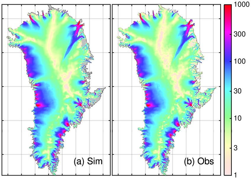
1170                                                         M. Rückamp et al.: Effect of overshooting on Greenland mass loss

2015). However, the statement of holding global temperature          ers, such as RACMO (Noël et al., 2018) or MAR (Fettweis
below 2 ◦ C implies keeping global warming below the 2 ◦ C           et al., 2017), with higher spatial and temporal resolution
limit over the course of the entire century and beyond, while        than GCMs. RCMs have been shown to be quite success-
efforts to limit the temperature increase to 1.5 ◦ C are often in-   ful in reproducing the current SMB of the GrIS. However,
terpreted as allowing for a potential overshoot before return-       as they are computationally expensive, an intermediate way
ing to below 1.5 ◦ C (Rogelj et al., 2015). Here we selected         would be more efficient to balance the computational costs
the Representative Concentration Pathway (RCP; Moss et al.,          and parameterization of processes, such as the surface energy
2010) 2.6 as the lowest emission scenario considered within          balance model of intermediate complexity (SEMIC; Krapp
CMIP5 and in line with a 1.5 or 2 ◦ C limit on global warm-          et al., 2017), which is employed in this study.
ing. Depending on the general circulation models (GCMs)                 Here we target RCP2.6 peak and decline scenarios in par-
considered, the global temperature change over time varies           ticular to study the GrIS response to overshooting with a nu-
considerably, although the political target is met by 2100.          merical ISM. The projections are driven with climate data
Whereas some models in RCP2.6 do not exceed the limit of             output from the CMIP5 RCP2.6 scenario provided by the
1.5 or 2.0 ◦ C global warming before 2100, other models do           ISIMIP2b project for different GCMs (Frieler et al., 2017).
and exhibit subsequent cooling (Frieler et al., 2017).               To obtain ice surface temperature and surface mass bal-
   While global temperature rise may be limited to 1.5 or            ance from the atmospheric fields, the surface energy balance
2 ◦ C by 2100, warming over Greenland is enhanced due                model SEMIC (Krapp et al., 2017) is applied. The SEMIC
to the Arctic amplification (Pithan and Mauritsen, 2014),            (Sect. 2.1) is driven off-line to the ISM and therefore the cli-
has already exceeded 1.5 ◦ C (relative to 1951–1980) in the          mate forcing is one-way coupled and applied as anomalies to
past decade (GISTEMP Team, 2018), and may exceed 4 ◦ C               the ISM. The advantage of this one-way coupling is the lower
by 2100. This yields more than 2 ◦ C warming by 2100 and             computational cost, allowing for reasonably high spatial and
could therefore have a considerable impact on ice sheet mass         temporal resolution of the ISM. In order to study the effect
loss over Greenland. This implies an enlargement of the abla-        of overshooting, we design an RCP2.6-like scenario without
tion zone and goes along with a decline in SMB. However, it          overshoot by manually stabilizing the forcing at 1.5 ◦ C.
is currently unclear how fast the GrIS could react to cooling           For modelling the flow dynamics and future evolution of
and recovery of SMB, as ice sheets also react dynamically to         the GrIS under RCP2.6 scenarios, the thermo-mechanical
atmospheric forcing.                                                 coupled Ice Sheet System Model (ISSM; Larour et al., 2012)
   Recent large-scale ice sheet modelling attempts to project        with a Blatter–Pattyn-type higher-order momentum balance
the contribution of the GrIS under RCP2.6 warming sce-               (BP; Blatter, 1995; Pattyn, 2003) is applied (Sect. 2.5). A
narios are very scarce. Fürst et al. (2015) conducted an ex-         crucial prerequisite for projections is a reasonable initial state
tensive study to simulate future ice volume changes driven           of the ice sheet in terms of ice thickness, ice extent, and ice
by both atmospheric and oceanic temperature changes for              velocities. Beside starting projections with the most realistic
all four RCP scenarios. For the RCP2.6 scenario they es-             setting, the prevention of a model shock after switching from
timate a sea-level contribution of 42.3 ± 18.0 mm by 2100            the initialization procedure to projections is very important.
and 88.2 ± 44.8 mm by 2300. The value by 2100 is in line             Both have been a major issue in the past, which gave rise to
with estimates given by the Fifth Assessment Report of the           an international benchmark experiment, initMIP Greenland
Intergovernmental Panel on Climate Change (IPCC AR5,                 (Goelzer et al., 2018), for finding optimal strategies to derive
IPCC, 2013). The AR5 range for RCP2.6 lies between 10                initial states for the ice velocity and temperature fields. Here,
and 100 mm by 2100 (the value depends on whether ice dy-             we apply a hybrid approach between a thermal paleo-spin-up
namical feedbacks are considered or not).                            and data assimilation.
   The GrIS response to projections of future climate change            Before driving the projections, the SMB forcing is vali-
are usually studied with a numerical ice sheet model (ISM)           dated thoroughly against RACMO. Then we explore the re-
forced with climate data. ISM response is subject to the dy-         sponse of the GrIS and its contribution to sea-level rise under
namical part and the surface mass balance (SMB). In the past,        the RCP2.6 scenario and a modified RCP2.6 scenario with-
ISMs often used the rather simple and empirically based pos-         out overshoot.
itive degree day (PDD) scheme, in which the PDD index
is used to compute melt, run-off, and ice surface tempera-
                                                                     2     Model description
ture from atmospheric temperature and precipitation (Huy-
brechts et al., 1991). One disadvantage of the PDD method            2.1    Energy balance model
is that the involved PDD parameters are tuned to correctly
represent present-day melting rates but may fail to repre-           Thermo-mechanical ISMs require the annual mean surface
sent past or future climates (Bougamont et al., 2007; Bauer          temperatures and annual mean surface mass balance of ice as
and Ganopolski, 2017). On one far end of model complex-              boundary conditions at the surface. To derive these ice-sheet-
ity, a regional climate model (RCM) resolves most processes          specific quantities, we use the surface energy balance model
at the ice–atmosphere interface and in the upper firn lay-           of intermediate complexity (SEMIC; Krapp et al., 2017). Al-

Earth Syst. Dynam., 9, 1169–1189, 2018                                                  www.earth-syst-dynam.net/9/1169/2018/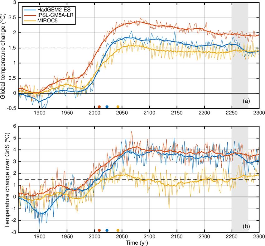
M. Rückamp et al.: Effect of overshooting on Greenland mass loss                                                                 1171

though we only apply SEMIC and do not adjust the param-            different GCMs were used in our study: IPSL-CM5A-LR
eters of SEMIC, SEMIC is described briefly. SEMIC com-             (L’Institut Pierre-Simon Laplace Coupled Model, version 5,
putes the mass and energy balance of snow and/or ice sur-          low resolution), MIROC5 (Model for Interdisciplinary Re-
face. In order to tune parameters for a number of processes,       search on Climate, version 5), and HadGEM2-ES (Hadley
Krapp et al. (2017) performed an optimization for the GrIS         Centre Global Environmental Model 2, Earth System). In-
forced with regional climate model data (MAR). These pa-           stead of the full acronyms we use IPSL, HadGEM2, and
rameters have been used in our study, too. The energy bal-         MIROC5 in the following text. The GCM output was pro-
ance equation reads as                                             vided and prepared by the ISIMIP2b project following a
                                                                   strict simulation protocol (Frieler et al., 2017). Figure 1a dis-
       dTs
ceff       = (1 − α) · SW↓ − LW↑ + LW↓ − HS − HL − QM/R ,   (1)    plays the temporal evolution of the annual global mean near-
        dt
                                                                   surface air temperature Ta for those GCMs for the historical
where α is the surface albedo that is parameterized with the       simulation up to 2005 continued with the RCP2.6 simulation
snow height (Oerlemans and Knap, 1998). The downwelling            up to 2299. Global mean temperature projections from IPSL,
shortwave SW↓ and downwelling longwave radiation LW↓ at            HadGEM2, and MIROC5 under RCP2.6 exceed 1.5 ◦ C rela-
the surface are provided as atmospheric forcing (Sect. 2.2).       tive to pre-industrial levels in the second half of the 21st cen-
The upwelling longwave radiation LW↑ is described by the           tury. While global mean temperature change returns to 1.5 ◦ C
Stefan–Boltzmann law. The latent HL and sensible HS heat           or even slightly lower by 2299 in HadGEM2, it only reaches
fluxes are estimated by the respective bulk approach (e.g.         about 2 ◦ C in IPSL by 2299. For MIROC5, temperature sta-
Gill, 1982). The residual heat flux QM/R is calculated from        bilizes at about 1.5 ◦ C during the second half of the 21st cen-
the difference of melting M and refreezing R and keeps track       tury. In order to determine the onset of overshoot we scan
of any heat flux surplus or deficit to keep the ice surface tem-   the historical and RCP2.6 scenarios of the individual GCMs
perature Ts below or equal to 0 ◦ C over snow and ice.             to identify the time when the global warming reaches 1.5 ◦ C
   The surface mass balance (SMB) in SEMIC is considered           in a 30-year moving window above pre-industrial levels. The
as follows:                                                        characteristic date of overshooting 1.5 ◦ C for HadGEM2 is
                                                                   by 2023; MIROC5 reaches this level by 2043, while IPSL
SMB = Ps − SU − M − R,                                      (2)
                                                                   reaches this point by 2009 (coloured dots in Fig. 1).
where Ps is the rate of snowfall and SU the sublimation rate,         The phenomenon that tends to produce a larger change in
which is directly related to the latent heat flux. The melt        temperature near the poles was termed polar amplification.
rate M is dependent on the snow height; if all snow has            Particularly, it enhances the increase in global mean air tem-
melted down, the excess energy is used to melt the under-          perature over Arctic areas (referred to here as Arctic amplifi-
lying ice. The refreezing R is calculated differently for avail-   cation). Generally, the CMIP5 models show an annual aver-
able meltwater or rainfall. Moreover, the porous snowpack          age warming factor over the Arctic between 2.2 and 2.4 times
could retain a limited amount of meltwater, while over ice         the global average warming (IPCC, 2013, Table 12.2). As
surfaces refreezing is neglected and all melted ice is treated     mechanisms creating the Arctic amplification may be repre-
as run-off. In SEMIC, the total melt rate and refreezing rate      sented to different extents in the GCMs, the level of future
are calculated from the available energy during the course of      amplification is different across the GrIS. The three GCMs
1 day. As the set of equations is solved using an explicit time    used in this study represent this trend to differing extents over
step scheme with a time step of 1 day, a parameterization          the GrIS1 (Figs. 1 and 2). For HadGEM2 and IPSL the Arctic
for the diurnal cycle (a cosine function) accounts for thawing     compared to global warming is amplified relatively similarly
and freezing over a day. This reduces complexity; the one-         (warming approximately 4 ◦ C relative to 1661–1860). In con-
layer snowpack model saves computational time and allows           trast, MIROC5 reveals a considerably lower Arctic amplifi-
for integration on multi-millennial timescales as opposed to       cation (warming approximately 3 ◦ C relative to 1661–1860).
more sophisticated multilayer snowpack models. Further de-         In terms of global and Arctic future annual mean near-surface
tails are given by Krapp et al. (2017).                            temperatures, MIROC5 offers the lowest and IPSL the high-
                                                                   est forcing.
                                                                      The ISIMIP2b atmospheric forcing data are CMIP5 cli-
2.2      Atmospheric forcing
                                                                   mate model output data that have been spatially interpo-
Here we targeted peak and decline scenarios in particular,         lated to a regular 0.5◦ ×0.5◦ latitude–longitude grid and bias-
temporarily exceeding a given temperature limit of global          corrected using the observational dataset EWEMBI (Frieler
warming to 2.0 ◦ C or even 1.5 ◦ C by the end of 2100. From        et al., 2017; Lange, 2018). To drive the SEMIC, we need
the official extended RCP2.6 scenarios (Meinshausen et al.,        to provide the atmospheric forcing (consisting of incoming
2011), we have selected GCMs which cover the CMIP5 his-
torical scenario, the RCP2.6 scenario until 2299, and reveal          1 For all occurrences, the area of the GrIS is defined as the ice
an overshoot in annual global mean near-surface temperature        mask provided from BedMachine Greenland (Morlighem et al.,
change relative to pre-industrial levels (1661–1860). Three        2014).

www.earth-syst-dynam.net/9/1169/2018/                                                 Earth Syst. Dynam., 9, 1169–1189, 2018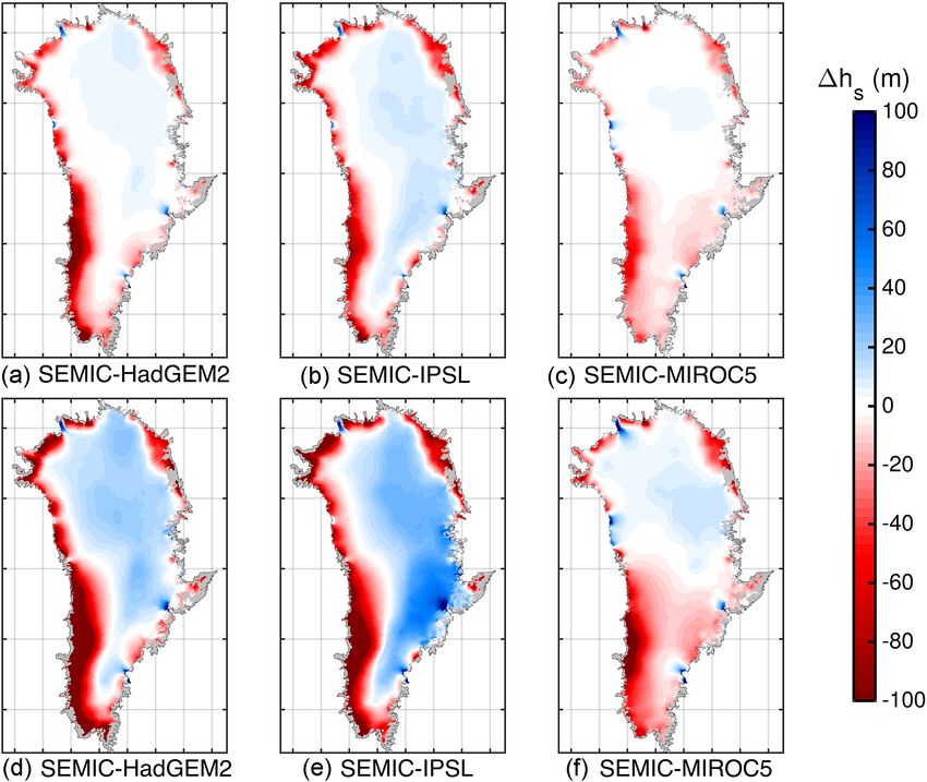
1172                                                         M. Rückamp et al.: Effect of overshooting on Greenland mass loss

Figure 1. Time series of annual global mean near-surface temperature change (a) and over the GrIS (b) for all three GCMs relative to 1661–
1880. The thick line is a 30-year moving mean. The coloured dots represent the onset years of overshooting 1.5 ◦ C in the global mean
near-surface air temperature in a 30-year moving window relative to pre-industrial levels. The light gray shaded area indicates the reused
time period for the scenario without overshoot.

shortwave radiation SW↓ , longwave radiation LW↓ , near-               tions for several quantities (·) denoted by (·)cor are initially
surface air temperature Ta , surface wind speed us , near-             performed. We follow the corrections proposed by Vizcaíno
surface specific humidity qa , surface air pressure ps , snowfall      et al. (2010),
rate Ps , and rainfall rate Pr ). These fields are available from
the output data of the three GCMs. SEMIC is driven by the              (·)cor = hSEMIC
                                                                                   s     − hGCM
                                                                                            s      γ(·) ,                           (3)
daily input of the GCMs, while the output is the cumulative
surface mass balance and the mean surface temperature over             with the lapse rates γ(·) shown in Table 1 and hSEMIC
                                                                                                                         s      equal
each year.                                                             to the ISSM ice surface elevation at the initial state. Subse-
   Given the differences in resolution between the GCMs and            quently, SEMIC computes the ice surface temperature Ts and
ISSM, a vertical downscaling procedure is applied to the at-           the SMB based on these corrected input values.
mospheric forcing fields. First, the atmospheric fields are in-           SEMIC is applied as developed by Krapp et al. (2017).
terpolated bilinearly from the GCM grid onto a regular high-           These authors perform a particle-swarm optimization to cal-
resolution 0.05◦ grid on which SEMIC is run. As a result,              ibrate model parameters for the GrIS and validate them
the output fields of SEMIC are conservatively interpolated             against the RCM MAR. We adopt their derived parame-
onto the unstructured ISSM grid. This two-step procedure is            ters here. The parameter tuning aimed to find a parameter
not necessary, but currently the easiest way from a technical          set which gives the best fit between SMB and ice tempera-
standpoint. For future applications we will avoid the interme-         ture Ts of SEMIC with only a limited number of processes
diate interpolation and run SEMIC directly on the unstruc-             and simpler parameterizations compared to a more com-
tured target ISSM grid. To account for the difference in ice           plex RCM. An RCM is typically validated against reanal-
sheet surface topography between GCMs and ISSM, correc-                ysis data and observations; therefore, we assume the tuned
                                                                       parameters are most reliable to represent the processes and

Earth Syst. Dynam., 9, 1169–1189, 2018                                                     www.earth-syst-dynam.net/9/1169/2018/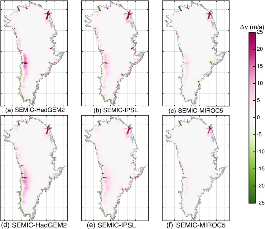
M. Rückamp et al.: Effect of overshooting on Greenland mass loss                                                                                  1173

Table 1. Lapse rates and height–desertification relationship for initial corrections of the GCM output fields near-surface air temperature Ta ,
precipitation of snow Ps , precipitation of rain Pr , and downwelling longwave radiation LW↓ used as input for SEMIC. Here, href = 2000 m
is the reference height and γp = −0.6931 km−1 is the desertification coefficient.

                       Variable    Lapse rates γ and desertification relationship                Reference
                       Ta          0.74 K/100 m                                                  Erokhina et al. (2017)
                       LW↓         2.9 W
                                        mh
                                           −2
                                                                       i                      Vizcaíno et al. (2010)
                       Ps , Pr     exp γp max hSEMIC ,       href − href ∀hGCM  ≤ href           Vizcaíno et al. (2010)
                                       h     s                        i s
                       Ps , Pr                 SEMIC
                                   exp γp max hs     ,       href − hGCM   ∀hGCM  > href         Vizcaíno et al. (2010)
                                                                     s        s

                                                                          tern of the SMB derived by forcing SEMIC with IPSL or
                                                                          MIROC5 is the same as when using HadGEM2. The compar-
                                                                          ison in Fig. 3 shows that the large-scale patterns of the SMB
                                                                          fields are in fairly good agreement, while the small-scale pat-
                                                                          tern and magnitudes of the GCM-based SMB do not match
                                                                          the RACMO2.3 SMB. Although the coarse GCM-based forc-
                                                                          ing has undergone a downscaling of particular fields and
                                                                          is processed in SEMIC with a higher resolution, the atmo-
                                                                          spheric fields over the ice sheet still lack details compared to
                                                                          an RCM. This is due to the fact that the forcing from a GCM
                                                                          implies different characteristics, like smoother gradients and
                                                                          a less-resolved geometry, compared to the RCM. The direct
                                                                          output of the SMB from SEMIC to the RACMO2.3 field
                                                                          has a misfit of about 2 m a−1 and a correlation coefficient
                                                                          of R 2 = 0.5. Additionally, the spatially integrated SMB for
                                                                          the averaged time period differs by up to 200 Gt a−1 . For
                                                                          HadGEM2, IPSL, and MIROC5 the values are 536, 496, and
                                                                          614 Gt a−1 , respectively. In contrast, the corresponding value
                                                                          for RACMO2.3 is 403 Gt a−1 . Therefore, we conclude that
                                                                          the absolute fields from SEMIC are not ideal for our purpose.
                                                                             Instead of using the absolute SEMIC output fields (SMB
Figure 2. Scatter plot of annual mean near-surface air temper-
                                                                          and Ts ) directly to force the numerical ice flow model ISSM,
ature change relative to pre-industrial levels over GrIS versus
annual global mean near-surface air temperature change for the            we rely on an anomaly method. The climatic boundary condi-
years 1861–2299. The gray line is the identity line.                      tions applied here consist of a reference field onto which cli-
                                                                          mate change anomalies from SEMIC are superimposed. The
                                                                          initialization of the ice flow model based on data assimilation
                                                                          (Sect. 2.6 below) makes it possible to use forcing data from
parameterizations within SEMIC. In terms of process de-                   high-resolution RCMs that were run on the same ice sheet
scription, the optimized SEMIC configuration leads to the                 mask and ice surface topography. As the reference SMB field
best possible SMB and Ts fields when MAR is used as forc-                 we choose the downscaled RACMO2.3 product (Noël et al.,
ing. If SEMIC is tuned with another RCM (e.g. RACMO or                    2018) whereby a model output was averaged for the time pe-
HIRHAM), the parameters will be different. Here, a separate               riod 1960–1990, denoted SMB(1960–1990)RACMO . The ref-
tuning for each GCM would be required due to the differ-                  erence period 1960–1990 is chosen as the ice sheet is as-
ences (e.g. the timing of maximum warming, the length of                  sumed close to steady state in this period (e.g. Ettema et al.,
an overshoot) among the GCMs used in this study. This basi-               2009). The climatic SMB that is used as future climate forc-
cally means compensating for too-low near-surface temper-                 ing reads
atures, for example, with SEMIC parameters, which would
offset the whole comparison of GCM forcing. Furthermore,                                           (1960−1990)
                                                                          SMBclim (x, y, t) = SMBRACMO           (x, y) + 1SMB(x, y, t),           (4)
these additional tuning steps would make the benefit of hav-
ing a semi-complexity model with low costs meaningless.                   with the anomaly defined as
   Figure 3 compares averaged SMB fields for the time pe-                                                                 (1960−1990)
riod 1960–1990 from RACMO2.3 and, as an example, the                      1SMB(x, y, t) = SMBSEMIC (x, y, t) − SMBSEMIC                 (x, y),    (5)
SMB derived by forcing SEMIC with HadGEM2. The pat-

www.earth-syst-dynam.net/9/1169/2018/                                                         Earth Syst. Dynam., 9, 1169–1189, 2018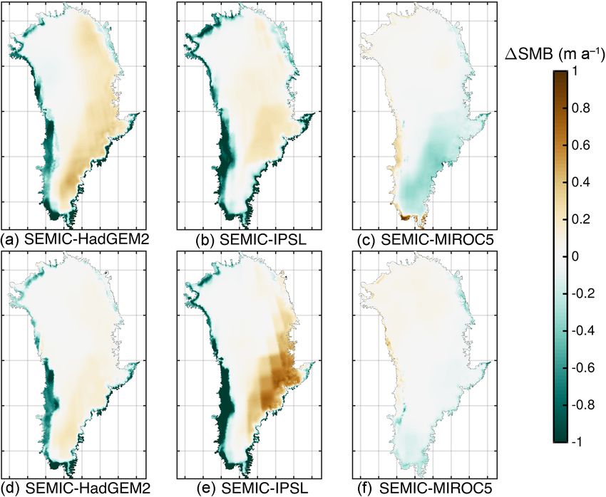
1174                                                        M. Rückamp et al.: Effect of overshooting on Greenland mass loss

Figure 3. Comparison of surface mass balance fields averaged for the time period 1960–1990; (a) surface mass balance derived by forcing
SEMIC with climate data from HadGEM2; (b) surface mass balance of RACMO2.3 (Noël et al., 2018).

where t = {1960, 1961, . . ., 2299}. Note that the histori-           2.3   Modified RCP2.6 scenario without overshoot
cal scenario is run from 1960–2005 and followed by the
RCP2.6 scenario from 2006–2299. In an ideal case, both                The global climate warming of the selected GCMs exceeds
reference terms SMB(1960–1990)RACMO and SMB(1960–                     the political target of 1.5 ◦ C during the 20th century, al-
1990)SEMIC will cancel out and the absolute climatic forc-            though RCP2.6 is the strongest mitigation scenario (Moss
ing SMBSEMIC (x, y, t) would remain. This is certainly not            et al., 2010). In order to estimate the effect of overshoot-
the case and the equation must be interpreted as having the           ing on the projected sea-level contribution from the GrIS we
RACMO2.3 reference field (with a good spatial distribution)           manually construct an RCP2.6-like scenario without an over-
as a background field with the trends from SEMIC superim-             shoot, assuming an immediate climate stabilization at that
posed.                                                                time when 1.5 ◦ C is reached. The characteristic time of over-
   The same equations hold for the temperature imposed on             shooting 1.5 ◦ C for HadGEM2 is by 2023; MIROC5 reaches
the ice surface. This ensures that the unforced control ex-           this level by 2043, while IPSL reaches this point by 2009.
periment produces identical behaviour for each GCM. Re-               Before reaching this threshold, the unaltered historical and
sults for future projections depend only on the atmospheric           RCP2.6 forcing is applied. The extension of the forcing from
GCM input or, similarly, SEMIC output and therefore the re-           these characteristic times is of crucial importance. To avoid
sults can be compared quantitatively. In the following text,          an unphysical step change, the climate in the repeated time
the constructed SMB fields according to Eq. (4) are referred          period should stabilize (i.e. no long-term trends in tempera-
to as SEMIC-HadGEM2, SEMIC-IPSL, SEMIC-MIROC5,                        ture change) close to 1.5 ◦ C warming. In order to account for
or in general as SEMIC-GCM.                                           decadal variability, i.e. extreme years, we reuse the climatic
   In the presented study, the ice flow model is forced               forcing fields from 2250–2280 until the end of the simula-
with the off-line-processed SEMIC output. As the ice sheet            tion (light gray shaded areas in Figs. 1 and 4). In this time
evolves in response to climate change, local climate feed-            window, the warming is close to 1.5 ◦ C and exhibits a fre-
back processes are not captured. Most importantly, this in-           quent number of extreme years. Other time windows might
cludes the interaction of the ice surface between air tempera-        also be feasible (e.g. the last 30 or 50 years), but will likely
ture and precipitation, which in turn affects the surface mass        not change the forcing substantially. In the following, the
balance. The SMB feedback process is considered with a dy-            modified RCP2.6-like scenario without overshoot is termed
namic correction to the SMBclim (see Sect. 2.7 below). This           RCP2.6 without overshoot.
correction is applied within ISSM and to the surface mass
balance term only.
                                                                      2.4   Assessment of SMB forcing

                                                                      We want to emphasize the fact that we do not intend to vali-
                                                                      date the energy balance model SEMIC itself, but rather as-

Earth Syst. Dynam., 9, 1169–1189, 2018                                                   www.earth-syst-dynam.net/9/1169/2018/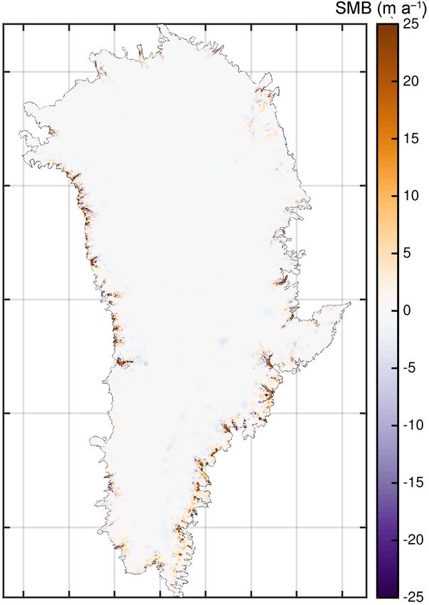
M. Rückamp et al.: Effect of overshooting on Greenland mass loss                                                                     1175

Figure 4. Time series of the annual mean integrated SMBclim (Gt yr−1 ) according to Eq. (4) for all three SEMIC-GCMs under RCP2.6
forcing (a) and RCP2.6 forcing without overshoot (b). The solid line is a 30-year and 15-year moving mean in (a) and (b), respectively. The
darker gray shading and black line represent the range and mean of SMB between 1981 and 2010 from Polar Portal (http://polarportal.dk/
forsiden/, last access: 8 October 2018). The dashed line shows the SMB time series of RACMO2.3 (Noël et al., 2018) from 1958–2016. The
coloured dots represent the onset years of overshooting 1.5 ◦ C in the global mean near-surface air temperature in a 30-year moving window
relative to pre-industrial levels. The light gray shaded time period indicates the repeated SMB forcing taken from the RCP2.6 scenario for
the scenario without overshoot.

sess whether the obtained SMB fields by forcing SEMIC                      For SEMIC-HadGEM2 the spatially integrated SMB re-
with the GCMs are plausible. In order to do so, the obtained            mains around 200 Gt a−1 after 2050. The SMB for SEMIC-
climatic SMBclim (Eq. 4), the resulting SMB patterns, and               IPSL recovers from 2050 onwards and shows an increase
time series are compared with other available datasets. Be-             from around 200 Gt a−1 to around 350 Gt a−1 by 2300.
side the spatial pattern of the surface mass balance, the time          SEMIC-MIROC5 reveals the lowest SMB change over time
series of the SMB over Greenland illustrates what the ice               and recovers after 2050 from 250 to 300–350 Gt a−1 by 2300.
sheet’s total surface gains and losses have been. The con-              By 2300, the SMB of SEMIC-IPSL and SEMIC-MIROC5 is
structed SMB forcings for the RCP2.6 scenario with and                  slightly below the present-day magnitude. However, the de-
without overshoot are shown in Fig. 4a and b, respectively.             cline of SMB for the RCP2.6 scenario roughly corresponds
The gray shaded box and black line depict the range and                 with MAR results forced with the GCM NorESM1-M under
the mean SMB between 1981 and 2010 from Polar Portal                    the RCP2.6 scenario (Fettweis et al., 2013 and last column
(http://polarportal.dk/forsiden/, last access: 8 October 2018)          in Table 2), although it is not strictly comparable because
derived from a combination of observations and a weather                they use different GCM climate data. They estimated a loss
model for Greenland (HIRLAM “newsnow”). The dashed                      of −124 ± 100 Gt a−1 in 2080–2099 relative to 1980–1999.
black line shows the results from the RACMO2.3 product.                    Table 2 shows the annual mean integrated SMB over the
The spatially integrated SMB magnitude of each SEMIC-                   entire GrIS for various periods. Averaged over most of the
GCM is consistent with the RACMO2.3 and Polar Portal                    periods, the annual mean integrated SMB is rather similar
data. The drop in SMB after 2000 is present in all three                among the models. Most obvious are the differences between
SEMIC-GCMs and RACMO2.3.                                                the SEMIC-GCMs for the period 1997–2016. The year 1997

www.earth-syst-dynam.net/9/1169/2018/                                                      Earth Syst. Dynam., 9, 1169–1189, 2018
1176                                                                  M. Rückamp et al.: Effect of overshooting on Greenland mass loss

Table 2. Annual mean integrated SMB (Gt yr−1 ) covering various periods. Time series of SMBclim for the SEMIC-GCMs are calculated by
Eq. (4) for the RCP2.6 scenario. The column “1.5 ◦ C reached” shows a 30-year mean at the characteristic time of overshooting 1.5 ◦ C. The
anomaly in SMB (1SMB) is in 2080–2099 with respect to 1980–1999.

          Model                     1960–1990        1960–1997        1997–2016         1981–2010    1960–2016    1.5 ◦ C       1SMB
                                                                                                                 reached
          RACMO2.3                     402.8            403.4            279.1               363.1     364.8        –                –
          Polar Portal                   –                –                –                  370        –          –                –
          MAR∗                           –                –                –                     –       –          –       −124 ± 100
          SEMIC-HadGEM2                400.0            391.2            277.0               358.1     355.2      170.0        −179.2
          SEMIC-IPSL                   408.9            412.5            332.8               403.7     382.2      363.9        −170.4
          SEMIC-MIROC5                 395.0            398.5            341.2               341.8     380.0      288.4         −80.9
        ∗ MAR forced with GCM NorESM1-M under the RCP2.6 scenario (Fettweis et al., 2013).

Figure 5. Inter-annual SMB variability for all SEMIC-GCMs (coloured lines) and RACMO2.3 (black line) calculated from consecutive
years; 1SMB = SMBt − SMBt−1 . The thick lines are a 30-year moving mean calculated from the yearly data (thin lines).

was identified as the critical time of Greenland’s peripheral                     2.5    Ice flow model
glacier and ice cap mass balance decrease (Noël et al., 2017).
For this period of declining SMB, the SEMIC-HadGEM2                               The ice flow and thermodynamic evolution of the GrIS
agrees well with the RACMO2.3 product, while the spatially                        are approximated using the finite-element-based ISSM. The
integrated SMBs for SEMIC-IPSL and SEMIC-MIROC5 are                               model has been applied successfully to both large ice sheets
∼ 40 and 50 Gt a−1 larger, respectively.                                          (Bindschadler et al., 2013; Nowicki et al., 2013; Goelzer
   For the available RACMO2.3 time series and the SEMIC-                          et al., 2018) and is also used for studies of individual
GCMs, we have computed the inter-annual SMB variabil-                             drainage basins of Greenland, e.g. the North-East Greenland
ity (Fig. 5). The SMB variability is similar to RACMO2.3                          Ice Stream (NEGIS) (Choi et al., 2017), Jakobshavn Isbræ
in terms of frequency and amplitude but is not coherent                           (Bondzio et al., 2016, 2017), and Store Glacier (Morlighem
among all models because the GCMs have their own inter-                           et al., 2016). Here, we use an incompressible non-Newtonian
nal variability. For the time period 1960–2016, the overall                       constitutive relation with viscosity dependent on tempera-
surface mass balance difference over the ice sheet between                        ture, microscopic water content, and strain rate, while ne-
SEMIC-GCM and RACMO2.3 is almost zero with −0.007,                                glecting the softening effect of damage or impurities. The BP
0.016, and 0.0200 m a−1 for SEMIC-HadGEM2, SEMIC-                                 approximation to the Stokes momentum balance equation is
IPSL, and SEMIC-MIROC5, respectively. These numbers                               employed in order to account for longitudinal and transverse
are in the same range as given by Krapp et al. (2017) for                         stress gradients.
the comparison between SEMIC and MAR.                                                ISSM is specified with kinematic boundary conditions at
                                                                                  the upper and lower boundary of the ice sheet. The upper
                                                                                  boundary incorporates the climatic forcing obtained from

Earth Syst. Dynam., 9, 1169–1189, 2018                                                               www.earth-syst-dynam.net/9/1169/2018/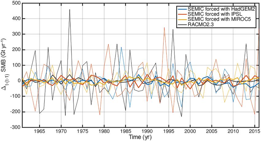
M. Rückamp et al.: Effect of overshooting on Greenland mass loss                                                              1177

SEMIC as explained above, i.e. the surface mass balance            cluster Cray CS400 computer, a simulation with an integra-
and ice surface temperature. The ice surface temperature is        tion time of 340 years requires ≈ 8 h on 16 nodes comprised
prescribed through Dirichlet boundary conditions. The base         of 36 CPUs.
of grounded ice is specified as both impenetrable with the
bedrock and in balance with the rate of basal melting. At the      2.6   Initial state
base of floating ice we use a Neumann boundary condition
that parameterizes the heat flux at the ice–ocean interface        Future projections of ice sheet evolution first require the de-
(Eq. 27 in Larour et al., 2012). The basal melt rate below         termination of the initial state. Different methods are cur-
ice shelves is parameterized with a Beckmann–Goosse rela-          rently used to initialize ice sheets, and it has been shown
tionship (Beckmann and Goosse, 2003). The melt factor is           that the initial state is crucial for projections of ice dynam-
roughly adjusted such that melting rates correspond to liter-      ics (Bindschadler et al., 2013; Nowicki et al., 2013; Goelzer
ature values (e.g. Wilson et al., 2017). Within this study the     et al., 2018). The recent initMIP–GrIS intercomparison ef-
basal melt rate is not a focus and hence the basal melt under-     fort (Goelzer et al., 2018) focuses on the different initializa-
neath floating tongues or vertical calving fronts of tidewater     tion techniques applied in the ice flow modelling community
glaciers are not changed. Once the pressure melting point at       and finds that none of them is the method of choice in terms
the grounded ice is reached, melting is calculated from basal      of a good match to observations and long-term continuity.
frictional heating and the heat flux difference at the ice–bed     All methods are required for modelling the projections of
interface. At the ice base, sliding is allowed everywhere and      the GrIS planned within the CMIP6 phase (Nowicki et al.,
the basal drag, τ b , is written using Coulomb friction:           2016) on timescales of up to a few hundred years. However,
                                                                   while inverse modelling is well established for estimating
τ b = −k 2 Nv b ,                                           (6)
                                                                   basal properties, the temperature field is difficult to constrain
where v b is the basal velocity vector tangential to the glacier   without performing an interglacial thermal spin-up.
base and k 2 a constant. The effective pressure is defined as         Here, we employ a hybrid approach between spin-up and
N = %i gH + %w ghb , where H is the ice thickness, hb the          an inversion scheme to estimate the initial state. For the hy-
glacier base, and %i = 910 kg m−3 and %w = 1028 kg m−3 the         brid initialization we make three basic simplifications: (1) the
densities for ice and seawater, respectively. We apply water       currently observed present-day elevation is taken as constant
pressure at the calving front of marine-terminating glaciers       for the entire glacial cycle. (2) The basal friction coefficient
and observed surface velocities (Rignot and Mouginot, 2012)        obtained from the inversion is taken as constant for the past
at the ice front of land-terminating glaciers. A traction-free     glacial cycle, and (3) the temperature changes from the GRIP
boundary condition is imposed at the ice–air interface.            record are applied to the whole ice sheet without spatial vari-
   Geothermal heat flows into the ice in contact with bedrock      ations.
and adjusts dynamically to the thermal state of the base (As-         The ice sheet geometry (bed, ice thickness, and ice
chwanden et al., 2012; Kleiner et al., 2015). The spatial pat-     sheet mask) is taken from the mass-conserving BedMachine
tern of the geothermal flux is taken from Greve (2005, sce-        Greenland dataset v2 (Morlighem et al., 2014). The geomet-
nario hf_pmod2).                                                   ric input for thickness and ice sheet mask is masked to ex-
   For all simulations, the ice front is fixed in time, and        clude glaciers and ice caps surrounding the ice sheet proper.
a minimum ice thickness of 10 m is applied. This implies           An initial relaxation run over 50 years assuming no sliding
that calving and melting exactly compensate for the outflow        and a constant ice temperature of −20 ◦ C is performed to
through the margins and initially glaciated points are not al-     avoid spurious noise that arises from errors and biases in
lowed to become ice free. However, regions that reach this         the datasets. A temperature spin-up is then performed using
minimum thickness have retreated. The grounding line is al-        this time-invariant geometry. As the computationally expen-
lowed to evolve freely according to a sub-grid parameteriza-       sive BP approximation is employed, mesh refinements are
tion scheme, which tracks the grounding line position within       made at certain points during the whole initialization proce-
the element (Seroussi et al., 2014).                               dure (see Table 3). The first mesh sequence starts 125 kyr be-
   Model calculations are performed on a horizontally un-          fore the present day and runs up to the year 1960, assuming
structured grid with a higher resolution, lmin = 1 km, in fast     a spatially constant friction coefficient k 2 = 50 s m−1 , and
flow regions and with a coarser resolution, lmax = 20 km, in       is forced with paleoclimatic conditions. The imposed pale-
the interior. The vertical discretization comprises 15 layers      oclimatic conditions consist of a multi-year mean from the
refined towards the base where vertical shearing becomes           years 1960 to 1990 of the RACMO2 product (Ettema et al.,
more important. The complete mesh comprises 574 056 el-            2009) and offset by a spatially constant surface temperature
ements. Velocity, enthalpy (i.e. temperature and microscopic       anomaly for the last 125 kyr based on the GRIP surface tem-
water content), and geometry fields are computed on each           perature history derived from the 118 O record (Dansgaard
vertex of the mesh using piecewise-linear finite elements.         et al., 1993). The initial ice temperature at 125 kyr before
The Courant–Friedrichs–Lewy condition (Courant et al.,             present is a steady-state temperature distribution taken from
1928) dictates a time step of 0.025 years. Using the AWI           a spin-up with time-independent climatic conditions from the

www.earth-syst-dynam.net/9/1169/2018/                                                    Earth Syst. Dynam., 9, 1169–1189, 2018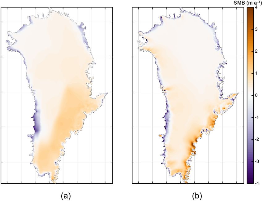
1178                                                         M. Rückamp et al.: Effect of overshooting on Greenland mass loss

Table 3. Mesh statistics.                                            tional shearing may be underestimated; this cannot be proven
                                                                     without any observations of basal velocities, which unfor-
       Mesh         lmin    lmax   Number of   Integration           tunately do not exist. However, for our projections on cen-
       sequence    (km)     (km)    elements       time in           tennial timescales this is a negligible effect (Seroussi et al.,
                                                  thermal            2013).
                                                   spin-up
                                                     (kyr)
                                                                     2.7   Synthetic and dynamic surface mass balance
       1              15    50      117 586           125                  parameterization
       2               5    50      192 220           125
       3             2.5    35      272 650            25            As we perform a one-way coupling of the climatic forcing,
       4               1    20      574 056            15            the SMB–elevation feedback needs to be considered. Here
                                                                     we rely on the dynamic SMB parameterization developed by
                                                                     Edwards et al. (2014a, b) and previously applied by Goelzer
reference period 1960–1990. The spin-up is done up to 1960           et al. (2013). This relationship was estimated from a set of
to start the projections before the critical time of Greenland’s     MAR simulations in which the ice sheet surface elevation
peripheral glacier mass balance decrease (Noël et al., 2017)         was altered. The parameterization assumes that the effect of
with an additional buffer of approximately 30 years.                 SMB trends follows a linear relationship:
   In the subsequent basal friction inversion, the ice rheol-        SMBdyn (x, y, t) = SMBclim (x, y, t)
ogy is kept constant using the enthalpy field from the end
of the temperature spin-up. The inversion approach infers                             + bi (hs (x, y, t) − hfix (x, y)) ,        (7)
the basal friction coefficient k 2 in Eq. (6) by minimizing a        where SMBdyn (x, y, t) and SMBfix (x, y, t) are the SMB val-
cost function that measures the misfit between observed and          ues with and without taking height changes into account, re-
modelled horizontal velocities (Morlighem et al., 2010). Ob-         spectively. The surface elevation changes are taken from the
served horizontal surface velocities are taken from Rignot           ISSM elevation hs (x, y, t) while running the simulation and
and Mouginot (2012). The cost function is composed of two            a reference elevation hfix (x, y). In our set-up the reference
terms which fit the velocities in fast- and slow-moving areas.       elevation corresponds to the ISSM ice surface elevation at
A third term is a Tikhonov regularization to avoid oscilla-          the initial state.
tions. The parameters for weighting the three contributions             In this parameterization the SMB gradient bi is depen-
to the cost functions are taken from Seroussi et al. (2013).         dent on both location and sign. It can take four values and
   The procedure for temperature spin-up and inversion is re-        a separation is made on the location relative to 77◦ N and
peated on the subsequent three mesh sequences. The repeated          on the sign of the SMB. This separates regions of largely
temperature spin-ups start 125, 25, and 15 kyr before 1990           different sensitivity, namely the ablation zone with a larger
and are again run up to the year 1960. The initial values for        gradient compared to the accumulation zone and a more
the temperature field at these times are taken from the respec-      sensitive ablation zone in the south compared to the north.
tive times from the previous mesh sequence; the basal fric-          While a complete uncertainty analysis is given by Edwards
tion coefficient is updated from the inversion on the previous       et al. (2014a), only the maximum likelihood gradient set,
mesh sequence. The mesh sequencing reduces the expense of            b = (bpN , bnN , bpS , bnS ), is used here:
initialization and produces a sufficiently consistent result in
terms of velocity and enthalpy. Note that mesh sequences 1–          bpN = 0.085 kg m−3 a−1 ,
3 are only used during initialization, while the final solution
                                                                     bnN = 0.543 kg m−3 a−1 ,
of mesh sequence 4 at year 1960 of this procedure is used as
the initial state for all projections presented below.               bpS = 0.063 kg m−3 a−1 ,
   Please note that similar results from this procedure have         bnS = 1.890 kg m−3 a−1 ,
been submitted to the ISMIP6 initMIP Greenland effort
(Goelzer et al., 2018), but the simulations were run with            where the subscripts (p, n) and the superscripts (N, S) in-
the geothermal flux distribution by Shapiro and Ritzwoller           dicate the evaluation of the SMB sign and the region sepa-
(2004) and additionally with a time-independent climate              ration, respectively. Please note that the employed relation-
forcing representing present-day conditions. However, by us-         ships with their parameters may change using a set-up from
ing the modified heat flux distribution by Greve (2005, sce-         SEMIC.
nario hf_pmod2), we found a generally better agreement                  A shortcoming of the performed hybrid initialization is
with measured basal temperatures at ice core locations. Basi-        that usually a fixed initial ice sheet causes a model drift
cally, the comparison of simulated to observed temperatures          when imposing the ice thickness equation. This is a result
at the ice base shows too-low temperatures for some loca-            of using an ice sheet that is not in equilibrium with the
tions. As the applied inversion technique for the friction co-       applied SMB and ice flux divergence. We utilize the lo-
efficient allows sliding everywhere, the portion of deforma-         cal ice thickness imbalance once the ice sheet is released

Earth Syst. Dynam., 9, 1169–1189, 2018                                                   www.earth-syst-dynam.net/9/1169/2018/
M. Rückamp et al.: Effect of overshooting on Greenland mass loss 1179
from its fixed topography from a single year unforced relax-
ation run, i.e. 1SMB(x, y, t) = 0 in Eq. (5). The resulting
∂H /∂t is subtracted as a surface mass balance correction,
SMBcorr (x, y), for all further runs (similar to Price et al.,
2011; Goelzer et al., 2018). However, instead of assuming
a zero SMB anomaly, one could calculate the anomaly with
a GCM input from the CMIP5 pre-industrial scenario. But
given the small temperature changes, the SMB anomaly will
be close to zero and the calculated ice thickness imbalance
is unlikely to be affected by it. However, the final SMB cor-
rection is on average 0.01 m a−1 , with 5 % of the total ice
sheet area having a correction of > 25 m a−1 , predominantly
at marine-terminated ice margins and ice streams (Fig. 6).
For these locations, the synthetic SMB correction can be
considered additional ice thinning or thickening from dy-
namic discharge that is not intrinsically simulated. A per-
formed control run with the imposed SMB correction ex-
hibits a small model drift in terms of sea-level equivalent
(SLE; black dashed line in Fig. 11 and Sect. 3.3).
The final surface mass balance that the numerical ice flow
model sees is composed of several components:
SMB = SMBclim (x, y, t) − SMBcorr (x, y) + SMBdyn (x, y, t). (8)
3 Results
3.1 Forcing fields
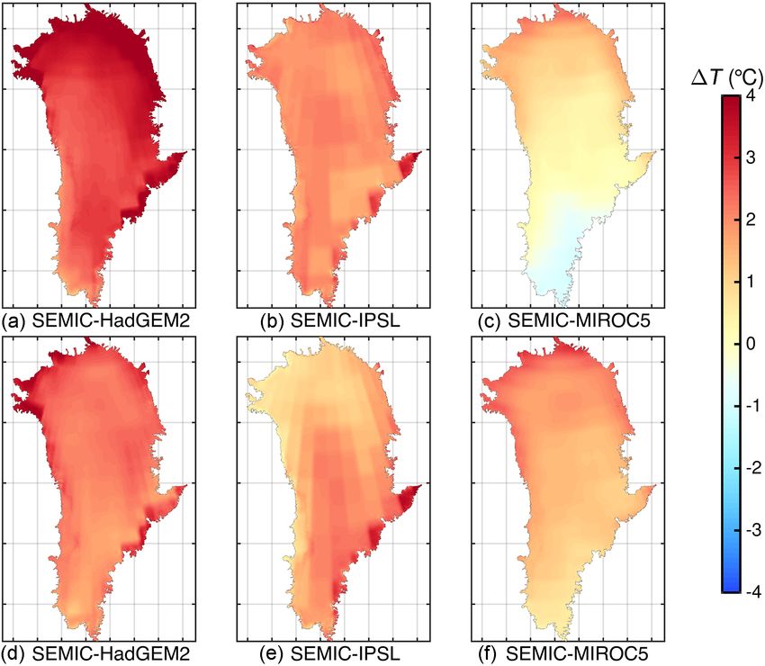
For the different GCMs used we compute ice surface temper- Figure 6. Synthetic surface mass balance SMBcorr calculated
from a single year unforced relaxation run (truncated at −25 and
ature Ts differences between 2100/2300 and 2000 as a multi-
25 m a−1 ). As the SMBcorr will be subtracted in Eq. (8) positive
year mean over 5 years to reduce the inter-annual variabil-
values represent enforced thinning, and negative values thickening.
ity (Fig. 7). HadGEM2 leads to an increase in temperatures
along the northern margins of up to 4 ◦ C. By 2100 the west-
ern areas and the vast majority of the ice sheet exceed 2 ◦ C
of warming. The only pronounced warming by 2300 is in contrast, MIROC5 produces less-pronounced warming over
the north-western regions, while the ice sheet surface tem- Greenland that is similar to the global mean warming but ex-
peratures decrease compared to 2100. IPSL exhibits a sig- hibits a plausible pattern of warming. IPSL is spatially and
nificantly different pattern with pronounced warming in the temporally experiencing the largest warming; however, the
centre (up to 3 ◦ C) and in the south-east (up to 4 ◦ C) of the ice distribution is not in agreement with the Arctic amplifica-
sheet. The northern areas reveal moderate warming around tion. Still, the assessment of the GCMs is in line with skill
1 ◦ C by 2100. The pattern is similar in 2300, with a moderate tests performed by Watterson et al. (2014) on a global scale.
cooling in the west compared to 2100. The least warming is They assigned skill scores by comparing individual GCM
found in MIROC5, which even exhibits cooling in the south- output data against reanalysis data. The analysis indicates
ern areas by about −1 ◦ C in 2100; warming of +1 ◦ C is only that all 25 models have a substantial degree of skill; how-
reached in the north. By 2300 the entire ice sheet experiences ever, HadGEM2 is ranked in the top, MIROC5 in the middle,
warming; however, this warming is quite moderate compared and IPSL in the lower part.
to the other two GCMs. The low magnitude of warming over Figure 8 presents, in a similar fashion as Fig. 7, the differ-
Greenland compared to global warming let us infer that the ences in SMB between 2100/2300 and 2000 as a multi-year
mechanisms of Arctic amplification are not well represented mean over 5 years each. The difference in SMB 2100–2000
in MIROC5. of SEMIC-HadGEM2 indicates a similar pattern as presented
Although we do not have a measure to judge future cli- by Krapp et al. (2017) using MAR (Fettweis et al., 2013): in-
mate warming trends, with respect to the Arctic amplifica- creasing SMB in the eastern part of the ice sheet with a max-
tion phenomena the most plausible distribution and mag- imum in the southern half of the ice sheet; at the ice sheet
nitude of surface warming is produced by HadGEM2. By margins ablation is increased. The same pattern is charac-
www.earth-syst-dynam.net/9/1169/2018/ Earth Syst. Dynam., 9, 1169–1189, 20181180 M. Rückamp et al.: Effect of overshooting on Greenland mass loss
Figure 7. Comparison of multi-year mean surface temperature (Ts ) differences between 2100–2000 (a–c) and 2300–2000 (d–f) for
(a, d) SEMIC-HadGEM2, (b, e) SEMIC-IPSL, and (c, f) SEMIC-MIROC5. The black contour line depicts the present-day ice mask.
teristic for 2300–2000, but with a slight decrease in melting minimum ice thickness and with that the ice extent in this
and accumulation. The SMB is reduced in the centre, leaving area is underestimated. However, ice surface elevations agree
a wide area with differences in SMB of 0.5 m a−1 and less. fairly well (Fig. 10b). In general large outlet glaciers like
The SMB difference of SEMIC-IPSL shows a similar pattern Kangerlussuaq, Helheim, and Jakobshavn Isbræ reveal lower
with enhanced amplitudes compared to SEMIC-HadGEM2, velocities in their fast termini that reflect the high RMS of
in particular, and the south-western margin; melting in the about 400 m a−1 (Fig. 10a). The RMS analysis here was done
south-west is increased by up to 1 m a−1 . In contrast, an SMB on the native grid with high resolution in fast flow regions
gain is concentrated in the centre-east by 2300. The most as- and the model was already run 40 years forward in time.
tonishing result is the 1SMB pattern in SEMIC-MIROC5: Compared to these values, the AWI-ISSM results on the reg-
increasing the SMB along the south-western and southern ular 5 km grid given in Goelzer et al. (2018) have a lower
margins in contrast to gently decreasing the SMB in the cen- RMS value of < 20 m a−1 .
tre of the ice sheet. By 2300 the 1SMB pattern changes
slightly and the SMB is decreasing in the south-western mar-
gins. The magnitude of 1SMB is lower compared to SEMIC- 3.3 Projections of mass change
HadGEM2 and SEMIC-IPSL.
After passing the assumed critical time of declining SMB of
the GrIS and the present-day state, the ice sheet experiences
3.2 Present-day elevation and velocities a warming and associated mass loss from a decline in sur-
face mass balance. Projections of the evolution of SLE of
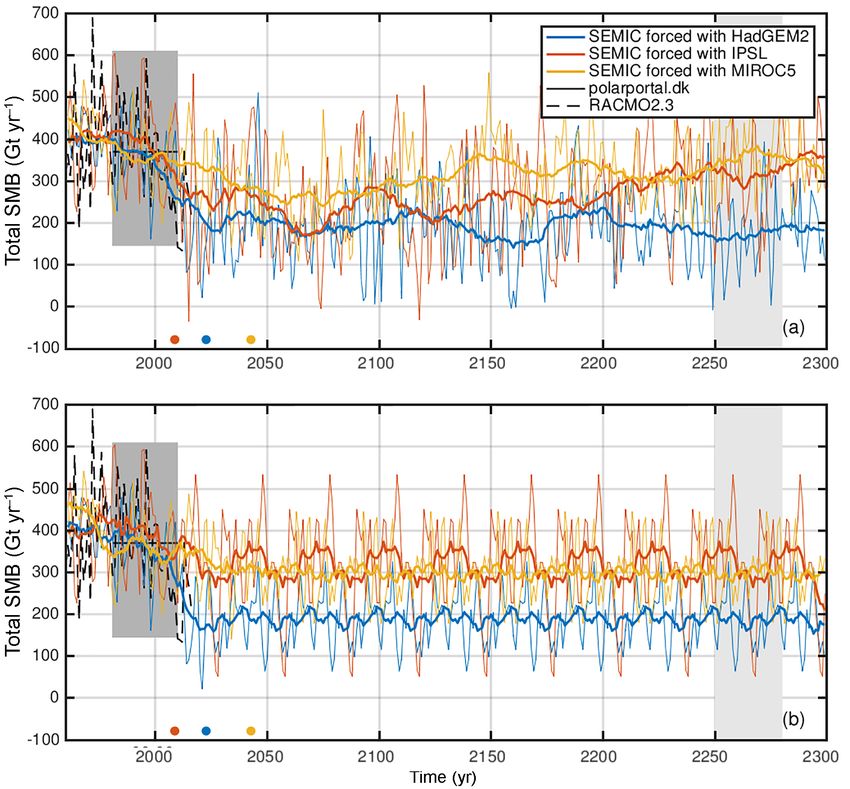
Figure 9 displays, as an example, the observed and simulated the ice sheet under the RCP2.6 scenario until 2100 and 2300
velocities for the year 2000 (defined here as present day) af- are shown in Fig. 11 for each GCM (solid lines) and Ta-
ter a period of forcing with SEMIC-HadGEM2 from 1960 ble 4. The simulated volume above floatation is converted
onwards. The resulting horizontal velocity field captures all into the total amount of global sea-level equivalent (SLE)
major features well, including the NEGIS. Outlet glaciers by assuming an ocean area of about 3.618 × 10⁸ km2 . Al-
terminating in narrow fjords in the south-eastern region are though the control run shows a small model drift in terms
resolved; however, slow-moving areas tend to retreat below of SLE (−1.4 and −0.7 mm for 2100 and 2300, respec-
Earth Syst. Dynam., 9, 1169–1189, 2018 www.earth-syst-dynam.net/9/1169/2018/M. Rückamp et al.: Effect of overshooting on Greenland mass loss 1181 Figure 8. Comparison of multi-year mean surface mass balance (SMB) differences between 2100–2000 (a–c) and 2300–2000 (d–f) for (a, d) SEMIC-HadGEM2, (b, e) SEMIC-IPSL, and (c, f) SEMIC-MIROC5. The black contour line depicts the present-day ice mask. Figure 9. Present-day velocities (year 2000) using SEMIC-HadGEM2: (a) observed velocities, (b) simulated velocities. Observed velocities: Rignot and Mouginot (2012). www.earth-syst-dynam.net/9/1169/2018/ Earth Syst. Dynam., 9, 1169–1189, 2018
1182                                                           M. Rückamp et al.: Effect of overshooting on Greenland mass loss

Figure 10. Scatter plots of the present-day state (year 2000) using the SMB forcing SEMIC-HadGEM2: (a) velocities, (b) ice surface
elevation. Blue and red dots in (a) represent floating and grounded points, respectively. Observed velocities: Rignot and Mouginot (2012);
observed surface elevation: Morlighem et al. (2014). The gray line is the identity line.

Figure 11. Sea-level equivalent (SLE, in millimetres) until the year 2100 (left panel) and 2300 (right panel) under RCP2.6 forcing (solid
lines) and RCP2.6 forcing without overshoot (dotted-dashed). Additionally, the control run (black dashed line) and the model mean and RMS
deviation from Fürst et al. (2015, Table B1) are shown. The coloured dots represent the onset years of overshooting 1.5 ◦ C in the global mean
near-surface air temperature in a 30-year moving window relative to pre-industrial levels.

tively), the RCP2.6 projected SLE is corrected by the control            mass; a change in trend with a minor increase between 2000
run. By 2100, the model range of Greenland sea-level con-                and 2015 and a steep increase from then on for SEMIC-
tributions is between 21.3 and 38.1 mm with an average of                HadGEM2 and SEMIC-IPSL; and the SLE increase for
27.9 mm and by 2300 between 36.2 and 85.1 mm with an av-                 SEMIC-MIROC5 is more gentle. The steep rise in SLE for
erage of 53.7 mm. Compared to Fürst et al. (2015) our mean               SEMIC-HadGEM2 and SEMIC-IPSL is linked to the steep
values are lower but still in their model range.                         reduction in SMB for both models at the same time. The kink
   The evolution of the mass change, expressed as sea-                   of SLE in SEMIC-HadGEM2 and SEMIC-IPSL around 2050
level equivalent (Fig. 11), shows distinct behaviours: be-               is caused by a positive SMB anomaly (compare Fig. 4).
tween 1960 and 2000 there is almost no change for SEMIC-                 SEMIC-MIROC5 also shows this peak in SMB, but slightly
HadGEM2 and SEMIC-IPSL, while SEMIC-MIROC5 gains                         later at around 2060. These short-term drops in SLE are

Earth Syst. Dynam., 9, 1169–1189, 2018                                                       www.earth-syst-dynam.net/9/1169/2018/
M. Rückamp et al.: Effect of overshooting on Greenland mass loss                                                                       1183

Table 4. Contribution of the Greenland ice sheet to global sea-level change by 2100 and 2300 in millimetres SLE under the RCP2.6 scenario
with and without overshoot.

                              Model/                          2100                               2300
                              study                    with            without            with            without
                                                     overshoot       overshoot          overshoot       overshoot
                              SEMIC-HadGEM2            38.1              29.6             85.1              66.9
                              SEMIC-IPSL               24.4               7.5             36.2               3.4
                              SEMIC-MIROC5             21.3              15.0             39.9              40.9
                              Average                  27.9              17.4             53.7              37.1
                              Fürst et al. (2015)   42.3 ± 18.0                –       88.2 ± 44.8             –

linked to positive anomalies in SMB. For SEMIC-HadGEM2
the ice sheet contribution until 2300 generally increases con-
tinuously, while for SEMIC-IPSL and SEMIC-MIROC5 the
increase levels off. This is an intriguing effect as SEMIC-
HadGEM2 and IPSL show a similar behaviour in terms of
warming over the GrIS (Fig. 1). In fact, the SMB of SEMIC-
IPSL recovers from 2050 onwards (Fig. 4), while the SMB
of SEMIC-HadGEM2 remains on a low level.
   For the RCP2.6 scenario without overshoot the behaviour
of SLE for SEMIC-HadGME2 is similar but with lower val-
ues. The SLE for SEMIC-MIROC5 is approximately 5 mm
lower by 2100 but approaches the same value at 2300 with-
out attaining a pronounced plateau. A striking feature is the
much lower SLE estimated from SEMIC-IPSL, which never
exceeds a value of 10 mm and gains mass from about 2225
onwards. The average SLE from all three GCMs is 17.4 mm
by 2100 and 37.1 mm by 2300, which is approximately one-
third less compared to the RCP2.6 scenario.                              Figure 12. Lag (j ) of projected sea-level rise per year under
   The observed sea-level contribution between 2002                      RCP2.6 forcing (coloured dots) and the modified RCP2.6 forcing
and 2014 is 0.73 mm a−1 (Rietbroek et al., 2016). In the                 without overshoot (coloured circles) as a mean for a time period
                                                                         similar to the observational period (2002–2014). The solid black
same period, the simulated contribution is only 0.16 mm a−1
                                                                         line indicates the observed value of 0.73 mm a−1 by Rietbroek et al.
for SEMIC-HadGEM2, 0.17 mm a−1 for SEMIC-IPSL, and
                                                                         (2016) and the dashed line the observed value of 0.40 mm a−1 cal-
the lowest for SEMIC-MIROC5 with 0.13 mm a−1 . In or-                    culated from RACMO2.3 for the period 2002–2014.
der to assess a potential temporal lag between the simu-
lated and observed value, mean values of similar periods
are calculated (Fig. 12). None of the models reaches the ob-
                                                                         3.4       Ice thickness change and dynamic response
served value (solid black line in Fig. 12); HadGEM2 reaches
a maximum value of 0.59 mm a−1 13 years later, SEMIC-                    Extensive marginal thinning is experienced by forcing the ice
IPSL a value of 0.48 mm a−1 12 years later, and SEMIC-                   sheet with SEMIC-HadGEM2 and SEMIC-IPSL (Fig. 13). In
MIROC5 a value of 0.36 mm a−1 40 years later. For the                    contrast to the mass loss near the margin, the interior shows
RCP2.6 scenario without overshoot, the values are smaller.               thickening; IPSL reveals more thickening in the interior.
Since a future ocean forcing and calving front retreat is not            Generally the large-scale pattern of marginal thinning and
considered here, the response of the ice sheet is likely un-             central thickening correlates with observations (Helm et al.,
derestimated. Comparing the sea-level contributions of each              2014) except that Petermann and Kangerlussuaq glaciers
SEMIC-GCM to the sea-level contribution of 0.4 mm a−1                    show an opposite trend. With a forcing of MIROC5 the pat-
calculated from RACMO2.3 for the same period (dashed                     tern of the elevation change is different with thinning in the
black line in Fig. 12) reveals a better agreement. SEMIC-                southern centre of the ice sheet; the northern centre experi-
HadGEM2 reaches this value 8 years later for the RCP2.6                  enced thickening. Although thinning occurs at the margin it
scenario with overshoot and 9 years later for the RCP2.6                 is less extensive compared to the other GCMs.
scenario without overshoot; SEMIC-IPSL reaches this value                   The response of ice velocities to RCP2.6 forcing is pre-
10 years later for RCP2.6 with overshoot.                                sented in Fig. 14, in which the change in horizontal sur-

www.earth-syst-dynam.net/9/1169/2018/                                                         Earth Syst. Dynam., 9, 1169–1189, 2018
You can also read