The PAU Survey: An improved photo-z sample in the COSMOS field
←
→
Page content transcription
If your browser does not render page correctly, please read the page content below
MNRAS 000, 1–20 (2020)                                                Preprint 23 July 2020             Compiled using MNRAS LATEX style file v3.0

                                               The PAU Survey: An improved photo-z sample in the COSMOS field

                                               Alex Alarcon1,2,3? , Enrique Gaztanaga2,3 , Martin Eriksen4 †, Carlton M. Baugh5,6 ,
                                               Laura Cabayol4 , Ricard Casas2,3 , Jorge Carretero4 †, Francisco J. Castander2,3 ,
                                               Juan De Vicente7 , Enrique Fernandez4 , Juan Garcia-Bellido8 , Hendrik Hildebrandt9 ,
                                               Henk Hoekstra10 , Benjamin Joachimi11 , Giorgio Manzoni5,6,12 , Ramon Miquel4,13 ,
                                               Peder Norberg5,6,12 , Cristobal Padilla4 , Pablo Renard2,3 , Eusebio Sanchez7 ,
arXiv:2007.11132v1 [astro-ph.GA] 21 Jul 2020

                                               Santiago Serrano2,3 , Ignacio Sevilla-Noarbe7 , Malgorzata Siudek4 , Pau Tallada-Crespí7 †
                                               (Author affiliations are listed after the references)

                                               23 July 2020

                                                                                      ABSTRACT
                                                                                      We present – and make publicly available – accurate and precise photometric redshifts in
                                                                                      the 2 deg2 COSMOS field for objects with iAB ≤ 23. The redshifts are computed using a
                                                                                      combination of narrow band photometry from PAUS, a survey with 40 narrow bands spaced
                                                                                      at 100Å intervals covering the range from 4500Å to 8500Å, and 26 broad, intermediate, and
                                                                                      narrow bands covering the UV, visible and near infrared spectrum from the COSMOS2015
                                                                                      catalogue. We introduce a new method that models the spectral energy distributions (SEDs) as a
                                                                                      linear combination of continuum and emission line templates and computes its Bayes evidence,
                                                                                      integrating over the linear combinations. The correlation between the UV luminosity and the
                                                                                      OII line is measured using the 66 available bands with the zCOSMOS spectroscopic sample,
                                                                                      and used as a prior which constrains the relative flux between continuum and emission line
                                                                                      templates. The flux ratios between the OII line and Hα , Hβ and OIII are similarly measured and
                                                                                      used to generate the emission line templates. Comparing to public spectroscopic surveys via
                                                                                      the quantity ∆z ≡ (zphoto −zspec )/(1+zspec ), we find the photometric redshifts to be more precise
                                                                                      than previous estimates, with σ68 (∆z ) ≈ (0.003, 0.009) for galaxies at magnitude iAB ∼ 18
                                                                                      and iAB ∼ 23, respectively, which is 3× and 1.66× tighter than COSMOS2015. Additionally,
                                                                                      we find the redshifts to be very accurate on average, yielding a median of the ∆z distribution
                                                                                      compatible with |median(∆z )| ≤ 0.001 at all redshifts and magnitudes considered. Both the
                                                                                      added PAUS data and new methodology contribute significantly to the improved results. The
                                                                                      catalogue produced with the technique presented here is expected to provide a robust redshift
                                                                                      calibration for current and future lensing surveys, and allows one to probe galaxy formation
                                                                                      physics in an unexplored luminosity-redshift regime, thanks to its combination of depth,
                                                                                      completeness and excellent redshift precision and accuracy.
                                                                                      Key words: photometric redshifts – galaxy evolution – cosmology

                                               1   INTRODUCTION                                                             cision. However, these are expensive to obtain: they require know-
                                                                                                                            ing the position of the object beforehand and a large exposure time,
                                               Redshift galaxy surveys can be broadly divided into two categories:
                                                                                                                            which makes it observationally inefficient to observe faint objects
                                               spectroscopic surveys and imaging surveys. The former obtains a
                                                                                                                            over a large area. Such surveys also suffer from incompleteness both
                                               high resolution spectra of the object within some wavelength cov-
                                                                                                                            because not all objects in the field are always targeted and also since
                                               erage, which is used to identify sharp features like emission and
                                                                                                                            a fraction of the measured spectra fail to provide an accurate redshift,
                                               absorption lines to nail the redshift of the object with very high pre-
                                                                                                                            for example for the lack of obvious emission or absorption features
                                                                                                                            in low signal-to-noise spectra, when only one line is observed, or
                                               ?
                                                                                                                            when there is a line confusion. In contrast, imaging surveys are
                                                  E-mail: alexalarcongonzalez@gmail.com (AA)                                able to obtain measurements of every object in the field of view at
                                               † Also at Port d’Informació Científica (PIC), Campus UAB, C. Albareda
                                               s/n, 08193 Bellaterra (Cerdanyola del Vallès), Spain
                                                                                                                            the same time from a set of bandpass filtered images, which allows

                                               © 2020 The Authors
2 A. Alarcon et al.
to cover large areas faster and to a greater depth. This happens at developed over the years to estimate their redshift distributions.
the expense of getting flux measurements with very poor spectral These can be broadly grouped as those which use angular cross-
resolution since the width of typical broad band filters is larger correlations with an overlapping tracer sample with well charac-
than 100nm, which makes the photometric redshift (i.e. photo-z) terised redshifts (clustering redshifts, see Newman 2008; Ménard
determination much less precise and sometimes inaccurate. et al. 2013; Schmidt et al. 2013; Gatti et al. 2018; Davis et al. 2017;
The precision of photometric redshift surveys can be improved Hildebrandt et al. 2017), those that model the galaxy spectral energy
with narrower bands and with a broader wavelength range coverage, distribution (SED) of each galaxy to connect their observed colours
and in recent years a new generation of multi-band photometric to redshift (e.g. Benítez 2000; Arnouts & Ilbert 2011; Tanaka 2015;
imaging surveys have emerged, for example, spanning from the Hoyle et al. 2018) and those that model the colour redshift rela-
ultraviolet to infrared (COSMOS, Ilbert et al. 2009), using sets of tion empirically using calibration samples (e.g. Cunha et al. 2012;
intermediate bands (ALHAMBRA, Molino et al. 2014) or a number De Vicente et al. 2016; Bonnett et al. 2016; Buchs et al. 2019;
of narrow band filters (PAUS, Eriksen et al. 2019). From the more Wright et al. 2019a). Each of these methods present different intrin-
precise photometric redshifts one can extract better measurements sic systematics and potential biases, and are typically best used in
of galaxy properties (luminosity, stellar mass, star formation rate) combination (e.g. Hildebrandt et al. 2017; Hoyle et al. 2018).
to probe and understand galaxy formation and galaxy evolution Direct or empirical calibration methods rely on galaxy sam-
physics with a denser sample, at higher redshifts, and with little ples where abundant redshift information is available, either through
selection effects. One can measure galaxy clustering in thin redshift spectroscopy or many band photometric redshifts. The former can
shells as a function of these intrinsic galaxy properties, measure be very accurate, but estimates are only available for a subset of
luminosity functions and star formation histories, or use galaxy- the sample, and the targeting strategy, quality selection and incom-
galaxy lensing to constrain the galaxy to halo connection in an less pleteness can introduce a statistical redshift bias with respect to the
explored luminosity-redshift regime. In particular, the Physics of the redshift of the full sample (Bonnett et al. 2016; Gruen & Brim-
Accelerating Universe Survey (PAUS) is an ongoing narrow band ioulle 2017; Speagle et al. 2019; Hartley et al. 2020; Wright et al.
imaging survey that intends to cover 100deg2 using 40 narrow band 2020). On the other hand, multi-band photometric surveys provide
filters, increasing the number of objects with subpercent redshift a complete redshift sample at the expense of degrading the redshift
precision by two orders of magnitude (Eriksen et al. 2019). The precision, and can be biased if the galaxy SED modelling is incor-
role of environment in structure formation is limited by the poor rect. The COSMOS field (Scoville et al. 2007) contains the most
redshift precision in broad band surveys and by the tiny area or widely used multiband redshift calibration survey, which provides
low density in spectroscopic surveys. The unique combination of a unique combination of deep photometric observations ranging
area, depth and redshift resolution from PAUS allows to sample from the UV to the infrared over an area of ∼ 2 deg2 , and several
with high density several galaxy populations, with which studies photometric redshift catalogues have been produced over the years
targeting nonlinear galaxy bias, intrinsic alignments, magnification (Ilbert et al. 2009, 2013; Laigle et al. 2016).
or density field reconstruction can be developed. Here, we combine the multiband photometry from Laigle et al.
On the other hand, imaging weak lensing galaxy surveys have (2016), hereafter COSMOS2015, with 40 narrow band filters from
entered the era of precision cosmology and have become one of the the PAUS survey (Padilla et al. 2019) which span the wavelength
most powerful probes for the ΛCDM cosmological model by mea- range from 4500Å to 8500Å. The unique PAUS photometric set is
suring the shape and position of hundreds of millions of galaxies. able to determine very precise photometric redshifts thanks to its
Current and future surveys such as the Dark Energy Survey (DES, exquisite wavelength sampling, which specifies precisely the loca-
Troxel et al. 2018; Abbott et al. 2018a,b), the Kilo-Degree Survey tion of the very sharp features in the galaxy SED (Eriksen et al.
(KiDS, Hildebrandt et al. 2017, 2020; Wright et al. 2019b, 2020), 2019, 2020). To estimate the photometric redshifts we develop an
Hyper Suprime-Cam survey (HSC, Aihara et al. 2018; Hikage et al. algorithm that models the galaxy SED as a linear combination of
2019), the Legacy Survey of Space and Time (LSST, LSST Dark continuum and emission line templates, and marginalises over dif-
Energy Science Collaboration 2012), or the Euclid mission (Lau- ferent combinations computing a Bayesian integral. Furthermore,
reijs et al. 2011) are reaching or will reach a point where systematic we calibrate priors between the continuum and emission line tem-
uncertainties limit the full exploitation of their statistical power. plates using a subsample with spectroscopic redshifts and the multi-
Among these, one of the most challenging systematic uncertainties band photometry. In Eriksen et al. (2019) a similar model (bcnz2)
is the characterisation of the redshift distribution of the weak lens- was used, where the best fitting linear combination of templates
ing tomographic samples, which contain millions of faint galaxies was calculated for each galaxy and model instead of the Bayesian
with a few colours measured using broad band filters. A correct integral. There, bcnz2 was used to measure redshifts using the 40
description of such redshift distributions is crucial to avoid intro- narrow bands from PAUS and a subset of 6 broad bands from COS-
ducing a bias in the cosmological inference (Huterer et al. 2006; MOS2015, for objects with iAB ≤ 22.5 until redshift zmax = 1.2.
Hildebrandt et al. 2012; Cunha et al. 2012; Benjamin et al. 2013; Here, we use a total of 66 bands which include 40 narrow bands
Huterer et al. 2013; Bonnett et al. 2016; Joudaki et al. 2017; Hoyle from PAUS and a combination of 26 narrow, intermediate, and
et al. 2018; Hildebrandt et al. 2017; Joudaki et al. 2019) and to broad bands from COSMOS2015, and we extend the magnitude
allow a robust comparison between cosmological parameters from and redshift limits to iAB ≤ 23 and zmax = 3. We make the redshift
weak lensing analysis and from the cosmic microwave background catalogue publicly available, including the redshift distribution of
(CMB, Planck Collaboration et al. 2018), especially when a number each object.
of recent studies suggest a mild tension between the values of cos- This paper is organised as follows. In section 2 we describe
mological parameters inferred for the early and late time universe the photometric data catalogues and the spectroscopic redshift cat-
(Joudaki et al. 2019; Asgari et al. 2019; Wright et al. 2020). alogue used in this work. Section 3 describes the methodology
The really large area and depth covered by these surveys makes used to describe the galaxy SED and infer the photometric red-
it unfeasible to measure spectroscopic redshifts for each galaxy of shift. Section 4 presents the primary photometric redshift results of
interest, which is why a number of alternative techniques have been this work. In section 5 we discuss more details of the analysis and
MNRAS 000, 1–20 (2020)PAUS+COSMOS photo-z sample 3
possible extensions for future work. We conclude and summarise in with sigma clipping. Cosmic rays are identified using a Laplacian
section 6. There are five appendices, which contain details of how to edge detection (van Dokkum 2001) and masked from the image.
download the catalogue (Appendix A), details of how we combine An astrometric solution is added to align the different expo-
heterogeneous data (Appendix B), details of the photo-z algorithms sures using scamp (Bertin 2011) by comparing to GAIA DR1 (Gaia
(Appendix C), the calibration of zero point offsets (Appendix D), Collaboration et al. 2016). The Point Spread Function (PSF) is
and the population prior on the models (Appendix E). modelled using psfex (Bertin 2011) in stars, where the star-galaxy
separation is done with morphological information using photome-
try from space observations of the COSMOS Advanced Camera for
Surveys (ACS, Leauthaud et al. 2007; Koekemoer et al. 2007). Pho-
2 DATA tometric calibration uses Sloan Digital Sky Survey (SDSS) stars
In this section we describe the data we are going to use through- that have been previously calibrated (Castander in preparation).
out. We will use narrow band photometry from the PAU Survey, a Each star brighter than iAB < 21 is fitted to obtain a probability for
combination of narrow, intermediate and broad bands coming from each SED in the Pickles stellar library (Pickles 1998) and Milky
various instruments publicly released by the COSMOS Survey, and Way extinction value using the u, g, r, i, and z broad bands (Smith
a spectroscopic redshift catalogue including measurements from et al. 2002). We generate synthetic narrow band observations from
several public redshift surveys. several star SEDs and weight them by their probability and compare
to the observations to obtain the zero point per star. All star zero
points are combined to obtain one zero point per image and narrow
2.1 PAUCam narrow band photometry band. This procedure also corrects for Milky Way extinction as the
synthetic narrow band fluxes are generated excluding the measured
The Physics of the Accelerating Universe Survey (PAUS) is an on- Milky Way extinction.
going imaging survey using a unique instrument, PAUCam (Padilla Narrow band photometry is obtained using the memba pipeline
et al. 2019), mounted at the William Herschel Telescope (WHT) (Multi-Epoch and Multi-Band Analysis, Serrano in preparation,
and located in the Observatorio del Roque de los Muchachos (La Gaztanaga in preparation). We rely on deep overlapping observa-
Palma, Canary Islands, Spain). PAUCam carries a set of 40 narrow tions from lensing surveys to provide a detection catalogue with
band (NB) filters with 12.5nm FWHM that span the wavelength high quality shape measurements to perform forced aperture pho-
range from 450nm to 850nm, in steps of 100nm. PAUS has been tometry. In the COSMOS field positions and shape measurements
collecting data since 2015 during several observing runs imaging from ACS are used. The half light radius, r50 , is used along with el-
five different fields: the COSMOS field (Scoville et al. 2007) and lipticity measurements from Sargent et al. (2007) and the PAUS PSF
the CFHT W1, W2, W3 and W4 fields1 . The PAU/CFHT fields are FWHM to determine the aperture size and shape to target 62.5% of
larger and represent the main survey, which is intended to observe the light, set to optimize the signal to noise. A flux measurement is
up to 100 deg2 , while the COSMOS field (2 deg2 ) has been targeted obtained for each individual exposure using this aperture measure-
as a calibration field since many photometric observations already ment and a background subtraction estimated from a fixed annulus
exist, ranging from ultraviolet all the way to far infrared, as well as of 30 to 45 pixels around the source, where sources falling in the an-
spectroscopic surveys with relatively high completeness and depth. nulus get sigma clipped (for more details of the annulus background
In this work we use the data collected in the COSMOS field from subtraction see Cabayol et al. 2019). Fluxes measured in different
campaigns between 2015 and 2017. exposures are corrected with the estimated image zeropoints and
get combined with a weighted average to produce a narrow band
coadded flux measurement.
2.1.1 Data reduction overview The data reduction pipeline propagates flags for each individual
At the end of each observing night, the data taken at WHT is exposure and object, and flagged measurements (indicating prob-
sent to Port d’InformaciÃş CientÃŋfica (PIC) for its storage and lems in the photometry) are not included in the weighted average.
processing (Tonello et al. 2019). The data reduction process starts We remove objects with fewer than 30 narrow band measurements.
with initial de-trending, where a number of signatures from the
instrument are removed from the images, using the nightly pipeline
(see Serrano in preparation, Castander in preparation for details). 2.2 COSMOS survey photometry
This includes removing electronic bias with an overscan subtraction, Along with the narrow band data described in the previous section,
correcting the gain from the different amplifiers and compensation we include photometry from several filters from the released COS-
from readout patterns using bias frames. A master flat is created MOS2015 catalog2 (Laigle et al. 2016), with filters from ultraviolet
from exposures of the dome with homogeneous illumination that to near infrared. Here we list the bands we use in this work, along
are taken every afternoon before the observation. It is used to correct with the original instrument/survey: NUV data from GALEX; u∗
the vignetting of the telescope corrector, among other effects such from the Canada-France Hawaii Telescope (MegaCam); (B, V, r, i + ,
as dead and hot pixels. Each individual narrow band filter is only z ++ ) broad bands, (I A427, I A464, I A484, I A505, I A527, I A574,
covering a single CCD, instead of a unique broad band that covers all I A624, I A679, I A709, I A738, I A767, I A827) intermediate bands
the focal plane, and the visible edges of the filters in the supporting and (N B711, N B816) narrow bands from Suprime-Cam/Subaru; Y
grid of the filter tray produced scattered light in the image edges. An broad band from HSC/Subaru; (Y , J, H, Ks ) from VIRCAM/VISTA
adjustment to the camera in 2016 significantly reduced this effect, (UltraVISTA-DR2); and (H, Ks ) data from WIRCam/CFHT.
which is partly mitigated by the pipeline by using a low pass filter We point the reader to (Laigle et al. 2016) and references
therein for a detailed overview of these observations and the data
1 http://www.cfht.hawaii.edu/Science/CFHLS/
cfhtlsdeepwidefields.html 2 ftp://ftp.iap.fr/pub/from_users/hjmcc/COSMOS2015/
MNRAS 000, 1–20 (2020)4 A. Alarcon et al.
reduction. We use the 3 00 diameter PSF homogenised coadded flux 8
×10−28 Example galaxy with iAB = 20.44, zspec = 0.231
Flux [erg s−1 cm−2 Å−1]
measurements available in COSMOS2015 and apply several cor-
rections as described and provided in the catalogue release. In par- 6
ticular, we correct for Milky Way dust extinction using the E(B −V) 4
value available for each galaxy and an effective factor Fx for each
2
filter x (see Table 3 and Equation 10 in Laigle et al. 2016) using
magcorrected = maguncorrected − E(B − V) ∗ Fx , (1) 5000 10000 15000 20000
Wavelength [Å] (Observer frame)
where the factors Fx are derived from the filter response function ×10−28
8
Flux [erg s−1 cm−2 Å−1]
and integrated against the galactic extinction curve (for a sense Narrow bands
of scale, FNUV ≈ 8.6 and Fz ++ ≈ 1.5). In addition, we remove 6 Intermediate bands
Broad bands
masked objects by using the flag parameter FLAG_PETER=0, as well 4
as objects identified as stars with TYPE!=1.
2
2.3 Combined photometric catalogue 4000 5000 6000 7000 8000 9000
Wavelength [Å] (Observer frame)
We combine the narrow band catalogue from PAUS and the photom-
etry from COSMOS2015 by matching objects by (ra, dec) position,
keeping objects within 1 00 radius. We restrict the analysis to objects Figure 1. The 66 photometric bands used in this work for an example galaxy
with an AUTO i band magnitude brighter than iAB ≤ 23, which we from the catalogue which has magnitude iAB = 20.44 and spectroscopic
redshift zspec = 0.231. Bands with qualitatively similar FWHM have the
obtain from Ilbert et al. (2009) (iAB is also the reference magnitude
same colour: broad bands in green, intermediate bands in yellow and narrow
in the PAUS data reduction). For objects fainter than this magnitude
bands in red. The horizontal width of the violin plots shows the FWHM of
the PAUS narrow band photometry has a typical signal to noise each filter, while the violin plot is a Gaussian distribution centered at the
well below 5 in all bands (see Figure 2 in Eriksen et al. 2019), measured flux and with variance equal to the measured flux variance plus an
but emission lines can still be significantly detected in the narrow extra systematic variance. Two blocks of emission lines are clearly visible in
band filters. We defer to future work how including PAUS NBs can the narrow bands, one containing the redshifted Hα line around λ ∼ 8100Å,
improve the photo-z performance in this fainter regime. The final and another containing the OIII doublet and H β around λ ∼ 6100Å.
unmasked catalogue contains 40672 galaxies.
The combination of heterogeneous photometry from different
instruments can be complicated and ultimately degrade the photo- of the catalogue has measurements available for all 66 bands, while
metric redshift performance of the catalogue if it is not performed 92% of objects have at least 65 bands measured. All objects have
consistently. While in the case of PAUS the flux measurement is measurements for the 12 intermediate bands and the four Y , J, H,
obtained from a variable aperture that targets 62.5% of the total Ks UltraVista NIR bands. All bands have measurements available
light of each galaxy, adapting to the galaxy’s apparent size and in at least 98% of the catalogue, except for the GALEX NUV band
taking into account the PSF of each individual image, the COS- which is missing in 23% of the objects.
MOS2015 photometry measures flux with a fixed aperture of 3 00 We make the photometric redshift catalogue publicly available
on PSF homogenised images. Therefore, each survey measures a along with the redshift distribution of each object (for details of the
different fraction of the light for each galaxy, which depends on its catalogue and how to download it see Appendix A).
apparent size. To deal with this effect, we have developed a self cali-
bration algorithm that benefits from the overlap between the Subaru
2.4 Spectroscopic data
r-band and the PAUS narrow bands. We introduce a synthetic Sub-
aru r-band flux, defined as a linear combination of narrow band flux To measure the precision and accuracy of the photometric red-
measurements, and find a rescaling factor for each object that we shifts we compare to spectroscopic redshifts. We use a compilation
apply to its narrow band photometry. In this way we homogenise the of public spectroscopic surveys (courtesy of Mara Salvato, private
photometry across surveys. We describe this method in Appendix B. communication) and we apply a quality flag to keep only objects
Finally, we note that the colours measured by each survey could also with a very reliable measurement. This compilation includes red-
be slightly different, but we will consider this is a negligible effect. shifts from the following instruments or surveys: zCOSMOS DR3
In addition, we add a systematic error to each band for all ob- (Lilly et al. 2009), C3R2 DR1&DR2 Masters et al. (2017, 2019),
jects, which accounts for any residual error that remains either from 2dF (Colless 1999), DEIMOS (Casey et al. 2017; Hasinger et al.
inaccuracies in the galaxy modelling, errors in the data reduction or 2018; Masters et al. 2019), FMOS (Kashino et al. 2019), LRIS (Lee
from joining inconsistent heterogeneous photometry from different et al. 2018), MOSFIRE (Kriek et al. 2015), MUSE (Rosani et al.
surveys. We add a 2% error to every band except for the UltraVista 2019), Magellan (Calabrò et al. 2018), VIS3COS (Paulino-Afonso
broad bands Y , J, H, Ks (5% error) and for the GALEX NUV band et al. 2018). Whenever more than one redshift measurement is avail-
(10% error), similar to those used by COSMOS2015 (priv. comm.). able for the same object we take the mean of all observations, and if
Figure 1 shows an example galaxy with the 66 photometric the multiple observations disagree by more than 0.002 in redshift,
bands we use in this work, coloured according to their width (broad we do not assign any spectroscopic redshift to that object (which
bands in green, intermediate bands in yellow and narrow bands in removes 95 objects in the spectroscopic catalogue). The spectro-
red). The horizontal width of the violins show the FWHM of each scopic catalogue has a total of 12112 objects with iAB ≤ 23 that
filter, while the violin is showing a Gaussian distribution centered match to the photometric catalogue. Figure 2 shows a summary of
at the measured flux and with variance equal to the measured flux the spectroscopic completeness of the catalogue as a function of iAB
variance plus the previously described extra systematic variance. magnitude, which stays above 40% for bright magnitudes and de-
Regarding the photometric band completeness, after flagging, 68% creases below 10% for the fainter objects considered, at iAB > 22.5.
MNRAS 000, 1–20 (2020)PAUS+COSMOS photo-z sample 5
the model at each redshift. The probability p( f |z, M) is given by
0.8
Spectroscopic completeness
∫
p( f |z, M) = p( f , α |z, M)dα
α
∫ (4)
0.6 = α, z, M)p(α
p( f |α α |z, M)dα
α
which is commonly referred as the Bayes evidence. We assume the
0.4 α, z, M) is given by a normal multivariate distribu-
likelihood p( f |α
tion,
0.2 α, z, M) = p
p( f |α
1
×
k σ( fk )
d
Î
(2π)
2 (5)
n
0.0
1 Õ © fk Õ t jk ª
17 18 19 20 21 22 23 exp −
− αj ®
2 k σ( fk ) j=1 σ( fk )
iAB « ¬
where k runs over the bands, j runs over the templates in the model
M, t jk is the flux for band k and template t j in the model, and σ( fk )
Figure 2. The spectroscopic completeness of the spectroscopic catalogue
used in this work as a function of iAB magnitude. The completeness is defined
is the measured flux error for band k.
as the fraction of objects in the catalogue which have a spectroscopic redshift The integral in Equation 4 requires that we specify a prior on
measured. The iAB magnitude is the reference magnitude in the PAUS data the model parameters p(α α |z, M). We distinguish between continuum
reduction, and is the AUTO i band magnitude from the Ilbert et al. (2009) and emission line SEDs in the prior,
catalogue.
α |z, M) =p(α0Cont |z, M)×
p(α
p(α1Cont |z, M)× (6)
Since the spectroscopic redshifts in this catalog come from high res-
p(α EL
|α0Cont, α1Cont, z, M)
olution instruments, we expect their precision error to be negligible
compared to the photo-z precision. However, there could be a sam- where we choose p(α0Cont, z, M) and p(α1Cont, z, M) to be top hat
ple of outlier spectroscopic measurements that we cannot flag, since functions,
the amount of duplicate spectroscopic measurements is very small.
p(α0Cont |z, M) ∝ Θ α0Cont Θ ∆0 − α0Cont
(7)
p(α1Cont |z, M) ∝ Θ α1Cont Θ ∆1 − α1Cont
3 METHODOLOGY
with Θ the Heaviside step function. Ideally, the prior for the contin-
In this section we describe the methodology used to model the uum amplitudes (Equation 7) should contain information about the
spectral energy distribution of a galaxy and obtain its redshift dis- luminosity function. We use a top hat prior between 0 and a max-
tribution. imum flux of (∆0, ∆1 ), which regards values outside these bounds
as unphysical. The values (∆0, ∆1 ) are set such that the maximum
flux does not exceed a given maximum luminosity threshold in the
3.1 Redshift distribution Subaru i-band, and the thresholds are calculated from the Subaru
i-band absolute magnitude which is derived from the data and the
We want to obtain the redshift probability distribution of a galaxy best model (see Section 3.3).
p(z| f ) from some flux observations f . To model the relation be- The prior probability term p(αEL |α0Cont, α1Cont, z, M) is one of
tween redshift and f we introduce a set of models denoted by {M } the key ingredients of our modeling, which constrains the colours
that can predict the fluxes f as a function of redshift. Therefore, we that arise from emission lines with respect to continuum flux. We
write estimate this prior using data, modeling a relation between the
Õ Õ
p(z| f ) = p(z, M | f ) ∝ p( f |z, M)p(z, M). (2) luminosity in the ultraviolet and the luminosity of the OII line,
{M } {M } which we describe in detail in Section 3.3.
We note that the Bayesian integral of Equation 4 is a gener-
Each model M is defined as a linear combination with parameters alization of previous work (see EAZY or BCNZ2 codes Brammer
{α j } of a particular set of spectral energy distributions {t} (SEDs), et al. 2008; Eriksen et al. 2019), which approximate the integral
Õ with the maximum likelihood
M(z) = α j (z) t j (z). (3)
j α max, z, M)
p( f |z, M) ≈ p( f |α (8)
The SED templates {t} can either be continuum templates of dif- where α max are the maximum likelihood values of the parameters
ferent galaxy populations or the flux from emission lines. In this within the positive orthant. We will use this approximation only
work we will use two continuum templates and one emission line when calibrating the prior for the emission lines and in the zero
template, so α = {α0Cont, α1Cont, αEL }. For details on the SED tem- point calibration step (see Section 3.3&3.4). To find the maximum
plates see the next subsections. We predict the colours at different likelihood values α max we will use the minimization algorithm
redshifts by redshifting the restframe SEDs and convolving with from bcnz2 (Eriksen et al. 2019). We reproduce this algorithm in
each filter accordingly. The amplitudes α are the free parameters of Appendix C1.
MNRAS 000, 1–20 (2020)6 A. Alarcon et al.
Groups of Continuum templates Extinction Laws Line λ[Å]
0) BC(0.008, 10), BC(0.008, 13) None Lyα 1215.7
1) BC(0.008, 8), BC(0.008, 10) None OII 3726.8
2) BC(0.008, 6), BC(0.008, 8) None OIII1 4959
3) BC(0.008, 4.25), BC(0.008, 6) None OIII2 5007
4) BC(0.008, 2.6), BC(0.008, 4.25) None Hα 6562.8
5) BC(0.02, 10), BC(0.02, 13) None Hβ 4861
6) BC(0.02, 8), BC(0.02, 10) None NII1 6548
7) BC(0.02, 6), BC(0.02, 8) None NII2 6583
8) BC(0.02, 4.25), BC(0.02, 6) None SII1 6716.4
9) BC(0.02, 2.6), BC(0.02, 4.25) None SII2 6730.8
10) Ell1, Ell4 None
11) Ell4, Ell7 None Table 2. List of emission lines included in the SED modeling. The lines are
12) Ell7, Sc None modeled with a Gaussian distribution with a width of 10Å centered around
13) Sc, SB0 None, Prevot the air wavelengths shown in the second column.
14) SB0, SB4 None, Prevot
None, Calzetti, Calz.+Bump1,
15) SB4, SB8 patrick & Massa 1986, 2007). We use two different amplitudes of
Calz.+Bump2
None, Calzetti, Calz.+Bump1, the bump following Laigle et al. (2016); Eriksen et al. (2019). We
16) SB8, SB11
Calz.+Bump2 generate a grid of templates with different E(B − V) values ranging
Table 1. List of continuum synthetic templates considered in different mod-
from 0.05 to 0.5 in steps of 0.05. We implement the IGM absorption
els M. We use continuum templates used in Laigle et al. (2016). The elliptical using the analytical correction from Madau (1995).
(Ell) and spiral (Sc) templates were generated by Polletta et al. (2007), while As mentioned in the previous section, each model M used in
the starburst models (SB) were generated by Bruzual & Charlot (2003). The this work contains two continuum templates. The complete list of
additional BC03 templates (BC) have their metallicity (Z) and age (Gyr) groups of two continuum templates is shown in Table 1. Some of
specified in parentheses, and were introduced in Ilbert et al. (2013). We the groups exist with different extinction laws created with a range
apply reddening to the continuum SEDs using extinction laws for spiral and of different E(B − V) values, as indicated in the table. We have
starburst templates, using a grid with 10 different E(B − V ) values spaced tested some combinations of three continuum templates but found
by 0.05 from 0.05 to 0.5 (see text for further details). In total, there are it to have little impact on the probability. The Bayes evidence has
97 combinations of continuum templates with different extinction laws and
preference for simpler models (an effect often named as Bayesian
extinction values.
Occam’s Razor, e.g. Ghahramani 2012) so that models with more
templates than needed to describe the data naturally get a lower
To efficiently compute the integral from Equation 4 we have im- probability. A group of at least two continuum templates guarantees
plemented a code based on a Gaussian integral algorithm from Genz a more continuous coverage in color space. We leave an exploration
(1992). Details of the algorithm are explained in Appendix C2&C3. of other combinations of templates, and the addition of different
synthetic templates to future work.
3.2 Galaxy SED
3.2.2 Emission lines
3.2.1 Continuum templates
All the models M include a third template which models the flux
Here we describe the continuum galaxy SED templates used in this
from emission lines. Table 2 shows a list of the lines we include and
work. We will use a library of synthetic SED templates generated
the wavelength on which they are centered. We model each line with
using recipes from Bruzual & Charlot (2003) and Polletta et al.
a Gaussian distribution of 10Å width (similar to lephare, Arnouts
(2007). This library, which is similar to the ones used in Arnouts
& Ilbert 2011, which accounts for some Doppler broadening due to
& Ilbert (2011); Ilbert et al. (2009, 2013); Laigle et al. (2016);
the galaxy’s rotational velocity). Therefore, our model will integrate
Eriksen et al. (2019), contains a set of Elliptical, Spiral and Starburst
over different combinations of continuum flux and emission line
synthetic templates. The templates in this library do not account
flux, with a greater ability to describe the observed flux of each
for the light attenuation due to the internal dust present in each
object than if we fixed these quantities.
galaxy. Generally, this effect varies in each galaxy. Following the
We build the emission line template tEL as
aforementioned references we model extinction using an extinction
law k(λ) and a color excess E(B − V) that adds this effect to the tEL ≡ ψ OII + βOIII ψ OIII + βHα ψ Hα + βHβ ψ Hβ (10)
template as
where
Fobserved (λ) = Fno dust (λ) × 10−0.4 E(B−V ) k(λ) . (9)
ψ OII ≡ OII + 2Lyα ;
We include this effect by modifying our default templates and gen- 1
erating new ones with different amounts of dust attenuation, since ψ OIII ≡ OIII1 + OIII2 ;
3 (11)
we cannot parametrize it linearly. For the starburst galaxies we will 1
use the extinction law from Calzetti et al. (2000), while for spirals ψ Hα ≡ Hα + 0.35( NII1 + NII2 + SII1 + SII2 );
3
we will model dust attenuation using the Prevot et al. (1984) law.
ψ H β ≡ Hβ ,
We will not add extinction to the reddest galaxy templates, like el-
lipticals templates. We include two modifications of the Calzetti law The notation OII, for example, in the above equation means a Gaus-
with an additional bump around 2175Å which was not prominent sian distribution centred at λ = 3726.8Å and 10Å width whose flux
in the original calibration of the law, but which has later been found integrates to 10−17 erg s−1 cm−2 , and similar for the other lines us-
in starburst galaxies (Stecher & Donn 1965; Xiang et al. 2011; Fitz- ing the wavelength values from Table 2. The parameters βOIII , βHα
MNRAS 000, 1–20 (2020)PAUS+COSMOS photo-z sample 7
and βHβ indicate the relative amount of flux between (ψ OIII , ψ Hα , From step (ii) we can also obtain absolute magnitudes for every
ψ Hβ ) and ψ OII and are determined from data (see section 3.3). galaxy, which we can correct for internal dust extinction using the
The term ψ OII contains the OII and Lyα lines. We include the best model (and the best extinction parameters). Of interest for us
Lyα line following previous photo-z analysis in the COSMOS field are the absolute magnitudes MNUV , MI , which stand for the GALEX
(Ilbert et al. 2009; Laigle et al. 2016) which used a fixed ratio of 2 NUV and Subaru i bands. In summary, this algorithm provides the
parameters (hαgEL i, hβgOIII i, hβgHα i, hβg β i,MNUV , MI ) for each of
between Lyα and OII. The Lyα line has a small impact since it only H
changes the flux of the Galex NUV filter for most of the galaxies the aforementioned galaxies.
in this analysis, which has the smallest signal to noise, and it only The distribution of MI peaks around magnitude -22 in our
enters the CFHT u band above redshift 2. The term ψ OIII contains sample, and we find no galaxies brighter than -26. We assume this
the OIII doublet, where the factor 13 comes from atomic physics (e.g. value to be the brightest magnitude a galaxy could be in this band,
Storey & Zeippen 2000). The term ψ Hα contains the Hα line and and set the upper limit of the top hat prior of the continuum templates
the NII and SII doublets, where the factor 13 also comes from atomic (∆0, ∆1 ) (Equation 7) to fulfil this condition at all redshifts.
physics (Storey & Zeippen 2000). Note that the Hα and NII lines are Figure 3 shows a density plot of the estimated mean values
hβg i, hβgHα i, hβg β i. For many of the galaxies, the measured
essentially blended together in our filter set, and we assign a fixed OIII H
ratio of 0.35 to the NII lines with respect to Hα , although this ratio signal-to-noise ratio on these parameters is low. Therefore, the den-
is smaller for lower stellar mass galaxies (e.g. Faisst et al. 2018). Hα sity plot is a convolution of some underlying distribution convolved
and SII doublet are distinguishable in different narrow bands until with this noise. We do not attempt to recover the true distribution
z ∼ 0.3, where they get redshifted outside of the PAUS narrow band in this work, but instead just measure the median and σ68 of the
coverage and become blended, so we model them together to have marginal noisy distribution, finding:
an homogeneous modeling at all redshifts. The Hβ line is modeled
separately in ψ Hβ . The emission line modeling presented here can be log10 (βgOIII ) = −0.50 ± 0.35
log10 (βg β ) = −0.56 ± 0.34
improved further using known relations: the BPT diagram (Baldwin H
(12)
et al. 1981) which establishes relations between the OIII, NII, Hα
and Hβ lines; the intrinsic case B recombination Balmer decrement log10 (βgHα ) = −0.08 ± 0.24
(Hα /Hβ ) = 2.86 (Storey & Hummer 1995; Moustakas et al. 2006); For each pair of continuum SEDs we add one emission line model
or modeling SII and Hα differently below and above z ∼ 0.3. with parameters βOIII , βHα , βHβ equal to the median values from
We defer a thorough exploration of these possibilities for future Equation 12. In order to account for the breadth of the distribution
work. Finally, we apply the same extinction law for the continuum we include 6 additional models per continuum group, each with one
templates and the emission line template, and modify the ratio of the β parameters set at a value two times the σ68 with respect
values according to the attenuation from extinction. to its median4 . In total, we have 679 different models M, each with
different continuum or emission line templates.
It is worth noting that step (i) in this section requires an initial
3.3 Prior on template parameters
assumption about the values of (βOIII , βHα , βHβ ) and the prior
In this section we describe how we estimate several parameters p(αEL |α0Cont, α1Cont, z, M). We initially fix these values to the line
in the model using spectroscopic data. To recap, we need to esti- flux ratio values from Ilbert et al. (2009). After the initial run, we
mate the parameters (∆0, ∆1 ) introduced in the continuum templates repeat the process to measure all of these parameters and calibrate
prior (Equation 7), describe the prior on the emission line tem- the prior (which is described later in this section). We repeat this
plate p(αEL |α0Cont, α1Cont, z, M) (Equation 6) and set the parameters process a couple of times, after which we find the values do not
(βOIII , βHα , βHβ ) from Equation 11. change. All the values reported in this section are the final values,
For each galaxy with a confident3 spectroscopic redshift in the which are used in the remainder of this work.
zCOSMOS-Bright spectroscopic catalog (see section 2.4), we carry
out the following steps 3.3.1 Prior p(αEL |α0Cont, α1Cont, z, M)
(i) Find the model M with the largest Bayes evidence at the Our model requires a prior on the emission line template free am-
galaxy’s spectroscopic redshift (Equation 4). plitude αEL . We will use the known correlation between the UV
(ii) For the most probable model M max , we find the maxi- luminosity of a galaxy and its OII emission line flux, which has been
mum likelihood parameters α max using the minimization algorithm used before in photometric redshift estimation (Kennicutt 1998; Il-
(Equation 8). bert et al. 2009), to build a model between αEL and the absolute
(iii) Subtract from the data the estimated continuum using the magnitude MNUV . We assume the following relation,
continuum α max parameters.
(iv) Produce Gaussian realizations centered at the subtracted flux p(η|MNUV ) ∼N (µ = aMNUV + b, σ = c),
(13)
using the measured flux error. For each realization, find the best fit η ≡ − 2.5 log10 (αEL ) − DM,
values for that galaxy: (αgEL , βgOIII , βgHα , βg β ). Note that since we
H
where DM is the distance modulus, N is a Gaussian distribution,
separately model additional internal dust reddening, these values and a, b, c are parameters to be determined from data. The pa-
are extinction free by definition. rameter η can be interpreted as an emission line absolute mag-
(v) Estimate the mean and standard deviation of the parameters nitude. Therefore, we assume there is a linear relation between
(αgEL , βgOIII , βgHα , βg β ) from the previous step.
H
4 These six additional models can be expressed as ([2,0,0],[0,0,2],[0,2,0],[-
2,0,0],[0,0,-2],[0,-2,0]), where for example [2,0,0] would mean (βg β , βgHα )
H
3 For this exercise we use only galaxies in the zCOSMOS-Bright DR3
release with a confidence flag c in the set: [3.x, 4.x, 2.4, 2.5, 1.5, 9.3, 9.4, are set at their median value, while βgOIII is set at at its median value plus
9.5, 18.3, 18.5] two times the measured σ68 .
MNRAS 000, 1–20 (2020)8 A. Alarcon et al.
−40
2
−42
η = −2.5 log10(αEL) − DM
log10(β Hα )
1
−44
0
−46
−1
−48
−2 0
−50
1 −52
1
0
log10(β Hβ )
0 −54
−28 −26 −24 −22 −20 −18 −16 −14 −12
−1 MNUV
−1
−2
−2
Figure 4. This figure shows the correlation between the OII line flux and the
−3
UV light as a density plot of the measured values of η ≡ −2.5 log10 (αEL ) −
−2 0 −1 0 1 DM and MNUV (Equation 13) for a subset of objects with spectroscopic
log10(β OIII) log10(β Hα ) redshift, where DM is the distance modulus. We expect these variables to be
correlated since the OII line flux is correlated with the ultraviolet luminosity
of a galaxy. We model this as a linear relation with an intrinsic Gaussian
Figure 3. This figure shows the line flux ratio between (mainly) the OIII, scatter, and find the most likely parameters of this model to calibrate the
Hα and H β lines with respect to the OII line, as the density plot of the log- prior between continuum and emission line templates, which is one of
arithmic measured values of β OIII , β Hα and β Hβ (Equation 10) which give the key ingredients in our redshift estimation model (see section 3.3). The
the relative amount of flux between different emission lines, as defined by measurements have been corrected for internal extinction.
Equation 11. The combined photometry of COSMOS and PAUS is used to
make the measurement for each object. We fit models of the emission lines
fore, we can hierarchically express the model as
to a continuum subtracted measured flux for a subset of objects with spec-
troscopic redshift, correcting for internal dust extinction (see section 3.3). Mg ∼ p(Mg |ξ)
ηg |Mg ∼ N (aMg + b, c) (14)
η̂g, M̂g |ηg, Mg ∼ N (ηg, σ(η̂)) × N (Mg, σ(M̂g )))
The likelihood function of the measured data p(η̂g, M̂g |θ, ξ) can
be obtained by integrating the complete data likelihood over the
missing data ηg, Mg
η and MNUV with an intrinsic scatter perpendicular to the cor- ∫ ∫
relation given by a normal distribution. In the model, the abso- p(η̂g, M̂g |θ, ξ) = p(η̂g, M̂g, ηg, Mg |θ, ξ) dηg dMg
lute magnitude MNUV is a function of the three free amplitudes, ∫ ∫
MNUV = MNUV (α0Cont, α1Cont, αEL ). Therefore Equation 13 de- = p(η̂g, M̂g |ηg, Mg )p(ηg |Mg, θ) (15)
scribes the probability of αEL given (α0Cont, α1Cont, z) which is our
probability p(αEL |α0Cont, α1Cont, z, M) for a given model M. × p(Mg |ξ) dηg dMg .
Figure 4 shows the relation between η and MNUV as a density In this work we will model p(Mg |ξ) with a mixture of K Gaussian
plot of the measured values for each galaxy, with αEL expressed distributions,
in units of 10−17 erg s−1 cm−2 . Similar to Figure 3, the plot does K
( )
Õ πk 1 (Mg − µk )2
not show the relation directly, since it is convolved with the mea- p(Mg |ξ) = exp − , (16)
τk2
q
2
surement noise of both variables. The inference of the parameters k=1 2πτk2
(a, b, c) in Equation 13 has to be done carefully to avoid introducing
where k πk = 1. Defining π ≡ (π1, . . . , πK ), µ ≡ (µ1, . . . , µK )
Í
a bias since the data is noisy in both axes (for more details see Kelly
2007; Hogg et al. 2010). and τ ≡ (τ1, . . . , τK ), note that we have ξ = (π, µ, τ). This mixture
We will infer the parameters θ ≡ (a, b, c) by writing the model is flexible enough to describe a wide variety of distributions,
likelihood of the observations given the parameters, following a and it is also convenient since it simplifies the mathematics for writ-
model similar to Kelly (2007). Let ηg , Mg be the true values ing the likelihood of the measured data (see Kelly 2007). Assuming
of the variables η, MNUV for galaxy g, and η̂g , M̂g be their the data for different galaxies is statistically independent, the full
noisy observational counterparts. We will assume Mg follows from data likelihood is the product of the measurement likelihood of each
a probability distribution p(Mg |ξ), where ξ are the parameters galaxy
of the distribution. The joint distribution of ηg and Mg is then n Õ
Ö K
πk
p(ηg, Mg |θ, ξ) = p(ηg |Mg, θ)p(Mg |ξ). We will assume a Gaus- p({η̂g }, {M̂g }|θ, ξ) =
2π|Vg,k | 1/2
sian and independent measurement error in η̂g and M̂g , so that g=1 k=1 (17)
p(η̂g, M̂g |ηg, Mg ) = p(η̂g |ηg )p(M̂g |Mg ) are two Gaussian distri-
1 −1 z
× exp − (zz g − ζk )Vg,k (z g − ζk )| ,
butions with means (ηg, Mg ) and variances (σ 2 (η̂), σ 2 (M̂g )). There- 2
MNRAS 000, 1–20 (2020)PAUS+COSMOS photo-z sample 9
with in the population can be jointly and hierarchically inferred along
zg = (M̂g, η̂g ), with the population’s distribution over different redshifts and mod-
els (e.g. Leistedt et al. 2016). This can be further extended to include
ζk = (aµk + b, µk ), a dependence of galaxy density on the line of sight position due to
(18)
a τk + c2 + σ 2 (η̂g )
2 2
aτk2 galaxy clustering (see Sánchez & Bernstein 2019; Alarcon et al.
Vg,k = .
aτk2 τk2 + σ 2 (M̂g )) 2019).
The redshift posterior of a galaxy is not unique since it depends
We fix the number of mixture Gaussians to K = 2 (although we on the population to which it belongs, or in other words different
have verified that the results for θ do not change if K = {2, 3, 4, 5}). galaxy sample selections will yield different p(z, M), and thus a
We maximize the likelihood in Equation 17 and find the most likely different posterior p(z| f ) for each galaxy. One proposed applica-
parameters θ ML to be tion of this redshift sample is to empirically calibrate the redshift
aML = 0.750 bML = −33.38 cML = 0.327 (19) distribution of galaxy samples from weak lensing surveys. Various
techniques exist (Wright et al. 2019a; Sánchez & Bernstein 2019;
We will use these values for all the results in this work. Finally, we Buchs et al. 2019; Alarcon et al. 2019; Sánchez et al. 2020) which
numerically integrate the prior, Equation 6, to compute the prior write a probability relation between the weak lensing galaxies and
normalisation, which is needed for the Bayes evidence, using a the galaxies from the calibration samples. The most correct output
Metropolis-Hastings integration algorithm. for such studies would be to produce and release the full likelihood
p(z, M | f ) for each galaxy, so that the redshift posterior and popu-
3.4 Systematic zero points offsets lation distribution can be inferred correctly for any galaxy sample.
This is impractical since the likelihood contains over a million val-
A common approach in the literature is to find systematic relative ues for each galaxy. Instead, we will compute and release a pseudo
(not global) zero-points between different bands before running the probability p̃(z| f ) defined as
photo-z algorithm (e.g. Benítez 2000; Coe et al. 2006; Hildebrandt Õ Õ
et al. 2012; Molino et al. 2014; Laigle et al. 2016; Eriksen et al. p̃(z| f ) = p(z, M | f ) ≈ p( f |z, M)p(M) (21)
2019). This attempts to optimise the colours predicted by the model {M } {M }
in comparison to the observed colours in the data. A zero point where we marginalize over the 679 models M, explicitly assuming
offset does not need to come from the zero point estimation itself, a uniform prior in redshift p(z|M). This probability can be inter-
but can also be due to an incorrect PSF modelling (Hildebrandt preted as an effective likelihood of a unique pseudo model, since it
et al. 2012), and from incorrect or missing templates. is a weighted likelihood over different models and has no explicit
We calibrate the systematic offsets with the same spectroscopic redshift prior. This effective likelihood p̃ can be used to infer the
catalogue described in section 3.3. We also use a similar algorithm. redshift distribution of a given population, and it is a good approx-
For every galaxy, we find the model M with the largest Bayes imation when all the p( f |z, M) which contribute significantly are
evidence M max and its most likely parameters α max . We build the similar, and given that p(M) is close to the real distribution of the
most likely fluxes Ti according to M max and α max . target population.
We assume the measured and predicted fluxes to be statistically We calibrate p(M) using a subset of the broad band colours
independent for every galaxy and band, and find the offsets {κ j } that we have available in data and the same colours predicted by each
maximise the likelihood model. The details are given in Appendix E.
ÖÖ
p({ fg }, {σg }, {Tg,k }|{κ j }) ≈ p( fg, σg, Tg,k |κ j )
k g
ÖÖ (20) 3.6 Comparison to previous models
= N ( fg κ j − Tg,k , κ j σg ).
The flux model developed here shares several elements with those
k g
implemented in bcnz2 (used in Eriksen et al. 2019, Er19) and le-
We apply the offsets (or factors for fluxes) to the data and run again, phare (used in Laigle et al. 2016, COSMOS2015), and it is worth
repeating the process until convergence. We exclude galaxies with highlighting some differences between them. Regarding the SED
a very bad fit ( χ2 > 120, with ∼ 63 degrees of freedom). The templates, the galaxy continuum templates and dust extinction laws
values of the offsets can be found in Appendix D, in Table D1 used are the same in all models, but the emission line templates
and Figure D1. It is worth noting that the calibration of the prior implementation differs. Er19 and COSMOS2015 create emission
described in section 3.3 and the offset calibration described in this line templates using fixed line flux ratios between several lines and
section depend on each other. We hierarchically run each part of the OII line, as measured by different spectroscopic surveys, and
the calibration, using the prior parameters and the zero point offsets originally collected in Ilbert et al. (2009). Here, we use a few differ-
from the previous step. We perform this a couple of times. ent values for the line flux ratios of line templates that contain the
OII, Hα , Hβ and OIII emission lines (Equations 10,11&12), mea-
sured directly from the 66 photometric bands and the best model.
3.5 Population prior and redshift posterior
In COSMOS2015 the emission line template was combined with
To obtain the redshift posterior p(z| f ) for each galaxy we need to the continuum template at three fixed amplitudes with respect to the
calculate Equation 2, which requires us to know the population’s continuum template, which were given by the correlation between
distribution over different redshifts and models, p(z, M). This quan- the UV luminosity and the OII line from Kennicutt (1998). Er19
tity is unknown a priori, and previous template codes and analysis left the amplitudes of the templates free (with a nonnegativity con-
have made different assumptions, such as assuming it is uniform, straint), and allowed for setups where the OIII doublet was an extra
or introducing analytical functions with hyperparameters calibrated template, separated from the other lines. Here, each model contains
with a spectroscopic population. Once a target population has been one emission line template, and its amplitude is marginalized with a
identified, the posterior on the redshift and model of each galaxy prior that also accounts for the distribution between UV luminosity
MNRAS 000, 1–20 (2020)10 A. Alarcon et al.
0.016 COSMOS2015 (Laigle et.al.)
This work: PAUS+COSMOS
0.014
0.012
0.010
σ68
0.008
0.006
0.004
0.002
18 19 20 21 22 23
Subaru iAB
3.0%
Outlier rate (|∆z| > 0.10)
2.5%
2.0%
1.5%
1.0%
0.5%
0.0%
18 19 20 21 22 23
Subaru iAB
Figure 5. The precision of the photo-z point estimates from this work (orange
lines) with respect to the spectroscopic redshift catalog. The top panel shows
the σ68 (Eq. 22) of the ∆ z ≡ (zphot − zspec )/(1 + zspec ) distribution as a
function of iAB magnitude, while the bottom panel shows the percentage of
galaxies classified as photo-z outliers, defined as objects that fulfill |∆ z | >
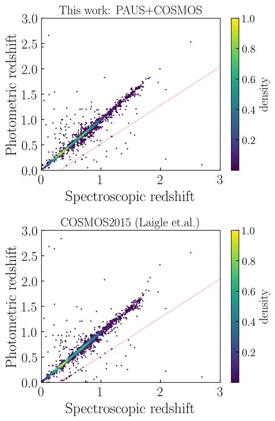
Figure 6. The scatter plot of the spectroscopic redshifts and the photo-z
0.1, also as a function of iAB magnitude. We compute the same statistics
point estimates of this work (top panel) and the photo-z point estimates
using the photo-z estimate from the COSMOS2015 public catalog (blue
from COSMOS2015 (bottom panel). Points are colored according to the
lines). We find a significant improvement in the redshift precision (lower
proximity (or density) of other nearby objects in this space. We find fewer
σ68 ) at all magnitudes considered in this work. The error bars are found by
outliers at ∆ z ≈ −0.24 (highlighted with a faint red line in both panels),
computing the dispersion of each metric when bootstrapping the objects in
which are consistent with a confusion between the OIII and Hα lines, where
each magnitude bin.
∆ z ≡ (zphot − zspec )/(1 + zspec ).
and the OII line, which we measure from the 66 photometric bands compare the redshift estimates with the spectroscopic catalog de-
(Equation 19). Additionally, COSMOS2015 included templates of scribed in section 2.4.
quasars and stars, unlike Er19 and this work.
Finally, in COSMOS2015 one single template which com-
bined continuum and emission line flux was fitted to the data, and 4.1 Photometric redshift precision
the best fitting amplitude was used to infer the likelihood at each
We define our photo-z point estimate zphot as the mode of the redshift
redshift; in Er19 the combination of several continuum templates (6
distribution of each galaxy p̃(z| f ) (Equation 21). When comparing
to 10) and several emission line templates (0 to 2) were maximized,
to the COSMOS2015 photo-z we will use the column PHOTOZ from
and the best fitting combination was used for the redshift inference;
their public catalog.
here, we marginalize over the amplitudes of two continuum tem-
To assess the accuracy and precision of the photo-z point esti-
plates and one emission line template with priors and compute the
mates with respect to the spectroscopic point estimates, we consider
Bayesian integral for the redshift inference.
the distribution of the following quantity: ∆z ≡ (zphot − zspec )/(1 +
zspec ). We define two metrics to assess the photo-z precision. One
is the central dispersion of the ∆z distribution, σ68 , defined as
4 RESULTS P[84] − P[16]
σ68 ≡ (22)
In this section we present the photometric redshift measurements 2
obtained using the model described in section 3, with the photom- where P[x] is the value of the distribution ∆z for the percentile x,
etry from PAUS and COSMOS described in section 2. We will which is more robust to outliers than the standard deviation of the
MNRAS 000, 1–20 (2020)You can also read