The global long-term microwave Vegetation Optical Depth Climate Archive (VODCA) - Earth System Science Data
←
→
Page content transcription
If your browser does not render page correctly, please read the page content below
Earth Syst. Sci. Data, 12, 177–196, 2020
https://doi.org/10.5194/essd-12-177-2020
© Author(s) 2020. This work is distributed under
the Creative Commons Attribution 4.0 License.

            The global long-term microwave Vegetation Optical
                     Depth Climate Archive (VODCA)
          Leander Moesinger1 , Wouter Dorigo1 , Richard de Jeu2 , Robin van der Schalie2 , Tracy Scanlon1 ,
                                     Irene Teubner1 , and Matthias Forkel1
            1 Department
                      of Geodesy and Geoinformation, Technische Universität Wien, Gußhausstraße 27–29,
                                               1040 Vienna, Austria
                       2 VanderSat, Wilhelminastraat 43A, 2011 VK Haarlem, the Netherlands

          Correspondence: Leander Moesinger (leander.moesinger@geo.tuwien.ac.at, vodca@geo.tuwien.ac.at)

                                  Received: 8 March 2019 – Discussion started: 15 April 2019
                     Revised: 12 November 2019 – Accepted: 1 December 2019 – Published: 30 January 2020

      Abstract. Since the late 1970s, space-borne microwave radiometers have been providing measurements of ra-
      diation emitted by the Earth’s surface. From these measurements it is possible to derive vegetation optical depth
      (VOD), a model-based indicator related to the density, biomass, and water content of vegetation. Because of
      its high temporal resolution and long availability, VOD can be used to monitor short- to long-term changes
      in vegetation. However, studying long-term VOD dynamics is generally hampered by the relatively short time
      span covered by the individual microwave sensors. This can potentially be overcome by merging multiple VOD
      products into a single climate data record. However, combining multiple sensors into a single product is chal-
      lenging as systematic differences between input products like biases, different temporal and spatial resolutions,
      and coverage need to be overcome.
         Here, we present a new series of long-term VOD products, the VOD Climate Archive (VODCA). VODCA
      combines VOD retrievals that have been derived from multiple sensors (SSM/I, TMI, AMSR-E, WindSat, and
      AMSR2) using the Land Parameter Retrieval Model. We produce separate VOD products for microwave obser-
      vations in different spectral bands, namely the Ku-band (period 1987–2017), X-band (1997–2018), and C-band
      (2002–2018). In this way, our multi-band VOD products preserve the unique characteristics of each frequency
      with respect to the structural elements of the canopy. Our merging approach builds on an existing approach that
      is used to merge satellite products of surface soil moisture: first, the data sets are co-calibrated via cumulative
      distribution function matching using AMSR-E as the scaling reference. To do so, we apply a new matching tech-
      nique that scales outliers more robustly than ordinary piecewise linear interpolation. Second, we aggregate the
      data sets by taking the arithmetic mean between temporally overlapping observations of the scaled data.
         The characteristics of VODCA are assessed for self-consistency and against other products. Using an auto-
      correlation analysis, we show that the merging of the multiple data sets successfully reduces the random error
      compared to the input data sets. Spatio-temporal patterns and anomalies of the merged products show consis-
      tency between frequencies and with leaf area index observations from the MODIS instrument as well as with
      Vegetation Continuous Fields from the AVHRR instruments. Long-term trends in Ku-band VODCA show that
      since 1987 there has been a decline in VOD in the tropics and in large parts of east-central and north Asia, while
      a substantial increase is observed in India, large parts of Australia, southern Africa, southeastern China, and
      central North America. In summary, VODCA shows vast potential for monitoring spatial–temporal ecosystem
      changes as it is sensitive to vegetation water content and unaffected by cloud cover or high sun zenith angles. As
      such, it complements existing long-term optical indices of greenness and leaf area.
         The VODCA products (Moesinger et al., 2019) are open access and available under Attribution 4.0 Interna-
      tional at https://doi.org/10.5281/zenodo.2575599.

Published by Copernicus Publications.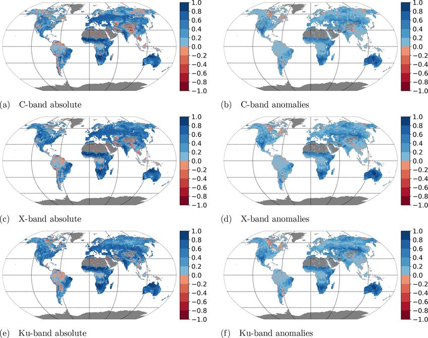
178                                                   L. Moesinger et al.: Vegetation Optical Depth Climate Archive (VODCA)

1   Introduction                                                    (TMI), and the Advanced Microwave Scanning Radiometer
                                                                    – Earth Observing System (AMSR-E) through the Land Pa-
                                                                    rameter Retrieval Model (LPRM; Owe et al., 2008). Their
Vegetation attenuates microwave radiation that is emitted or        methodology was inherited from the methodology used to
reflected by the Earth surface. The degree of attenuation can       produce the first long-term satellite-based climate data record
be derived from passive and active microwave satellite ob-          of soil moisture within the Climate Change Initiative of the
servations and is commonly referred to as vegetation op-            European Space Agency (ESA CCI Soil moisture; Dorigo
tical depth (VOD) (Jackson and Schmugge, 1991; Vreug-               et al., 2017, 2012; Liu et al., 2011c, 2012; Gruber et al.,
denhil et al., 2016). The amount of attenuation depends on          2019). In their methodology, all available observations were
various factors, e.g. the density, type, and water content of       harmonized with respect to C-band (6.9 GHz) VOD obser-
vegetation and the wavelength of the sensor (Jackson and            vations from AMSR-E, which was assumed to provide the
Schmugge, 1991; Owe et al., 2008). Short wavelengths ex-            highest-quality observations (Liu et al., 2012). Only in peri-
perience a higher attenuation by vegetation (and hence re-          ods where AMSR-E C-band observations were not available,
late to higher VOD values) than longer ones (Liu et al.,            were other products used instead. This approach ignores the
2009; Owe et al., 2008; Rodríguez-Fernández et al., 2018).          fact that in a statistical sense a high-quality product can be
As a consequence, VOD estimates from long wavelengths               fused with a low-quality product to create a product with a
are generally more sensitive to deeper vegetation layers (e.g.      higher quality than either of the original products. This was
stem biomass) while VOD estimates from short wavelengths            systematically demonstrated for the merging of two level 2
are more sensitive to leaf moisture content (Chaparro et al.,       soil moisture products (Gruber et al., 2017). Since the re-
2018; Tian et al., 2018; Fan et al., 2018; Konings et al., 2019).   lease of the multi-satellite VOD product by Liu et al. (2011a),
VOD increases with the vegetation water content (VWC)               significant progress has been made towards a better under-
(Jackson and Schmugge, 1991) and therefore is related to the        standing of the VOD signal. It was shown that the individ-
above-ground dry biomass (AGB) (Liu et al., 2015) and its           ual bands also carry valuable information for different appli-
relative water content (RWC) (Momen et al., 2017).                  cations (Teubner et al., 2018; Chaparro et al., 2018), which
   Satellite-derived VOD has a wide range of potential ap-          demonstrates the need for frequency-specific VOD data sets.
plications, including biomass monitoring (Liu et al., 2015;         In addition, new sensors were launched, allowing the obser-
Brandt et al., 2018b), drought monitoring (Liu et al., 2018),       vational VOD records to be extended to the running present.
phenology analyses (Jones et al., 2011), and estimating the            In this paper, we present a new series of long-term, har-
likelihood of wildfire occurrence (Fan et al., 2018; Forkel         monized VOD climate data records, called the VOD Cli-
et al., 2017, 2019). VOD also correlates with various optical       mate Archive (VODCA), which are derived from multiple
remote sensing indicators of vegetation greenness like nor-         single-sensor level 2 products. VODCA uses a similar core
malized difference vegetation index (NDVI), enhanced vege-          methodology as in Liu et al. (2011a) and in ESA CCI Soil
tation index, normalized difference water index (Grant et al.,      Moisture (Gruber et al., 2019) but incorporates the latest in-
2016), and leaf area index (LAI) (Vreugdenhil et al., 2017)         sights into VOD and climate data record production gath-
and hence also relates to plant productivity (Teubner et al.,       ered during the last few years, and it introduces recent satel-
2018, 2019). VOD has some distinct advantages over opti-            lite missions. We combine VOD observations from SSM/I,
cal vegetation indexes for vegetation monitoring, such as a         TMI, AMSR-E, WindSat, and AMSR2 into global, harmo-
slower saturation and the resulting higher sensitivity to high      nized long-term VOD products at a 0.25◦ spatial sampling
biomass (Liu et al., 2015) or the ability to be retrieved de-       and covering the period 1987–2018. First, we describe the
spite cloud cover (Liu et al., 2011a) which are both advanta-       input VOD data sets, followed by an overview of the fusion
geous for monitoring tropical forest regions (van Marle et al.,     methodology. We then describe the main characteristics of
2016).                                                              the merged data sets in terms of spatial and temporal cover-
   VOD products have been derived from multiple space-              age and patterns and their random error characteristics. We
borne microwave sensors that have been in orbit since the           check the spatio-temporal characteristics for plausibility by
late 1970s (Owe et al., 2008). These sensors have varying           comparing them to those of related satellite-derived biogeo-
lifetimes and characteristics, resulting from differences in        physical products and complement the data set assessment
microwave frequency used, measurement incidence angles,             by a trend analysis. We conclude the paper with a discussion
orbit characteristics, radiometric quality, and spatial foot-       on current limitations and ways forward.
prints. This complicates their joint use in studying long-term
VOD dynamics. To overcome this issue, Liu et al. (2011a)
proposed a long-term (1987–2008) harmonized multi-sensor
VOD data set by merging VOD products derived from the
Special Sensor Microwave/Imager (SSM/I), the Microwave
Imager on board the Tropical Rainfall Measuring Mission

Earth Syst. Sci. Data, 12, 177–196, 2020                                             www.earth-syst-sci-data.net/12/177/2020/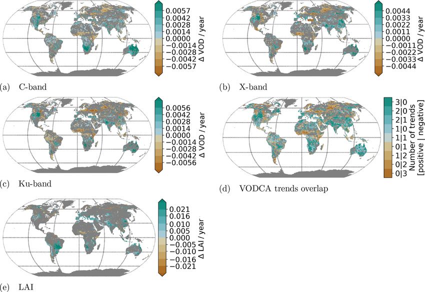
L. Moesinger et al.: Vegetation Optical Depth Climate Archive (VODCA)                                                       179

2     Input data                                                   2.1.2   Sensor specifications

2.1     Vegetation optical depth data sets                         The used VOD data sets were derived from brightness tem-
                                                                   perature measurements of various space-borne sensors active
2.1.1    The Land Parameter Retrieval Model (LPRM)
                                                                   since 1987 (Table 1).
LPRM v6 (van der Schalie et al., 2017; Owe et al., 2008;              The Advanced Microwave Scanning Radiometer (AMSR-
Meesters et al., 2005) is based on a radiative transfer model      E) on board Aqua retrieved microwave observations from
first proposed by Mo et al. (1982), and it simultaneously re-      2002 to 2011 in six bands, of which we only consider
trieves soil moisture and VOD from vertical and horizontal         the C-, X-, and Ku-bands. Their spatial footprints are
polarized microwave data. The model assumes that the Earth         75 km × 43 km, 51 km × 29 km, and 27 km × 16 km respec-
emits microwave radiation depending on its surface temper-         tively. AQUA is on a sun-synchronous circular orbit, passing
ature Ts and emissivity e, which is a function of its dielectric   the Equator at 13:30 ascending and 01:30 descending mode
constant k, which in turn is dependent on the surface soil         (Knowles et al., 2006; Kawanishi et al., 2003).
moisture. Part of this radiation is then absorbed or scattered        The Advanced Microwave Scanning Radiometer 2
by water in the vegetation depending on its transmissivity         (AMSR2) is an improved version of AMSR-E on board
0 and single-scattering albedo w, while the vegetation itself      GCOM-W1 continuing AMSR-E’s measurements since
also emits radiation depending on its temperature Tv . The re-     2012 with similar bands, orbit, and overpass times but
sulting brightness temperature Tb measured at the sensor can       with a slightly higher spatial resolution: 62 km × 35 km,
then be modelled as                                                42 km × 24 km, and 22 km × 14 km, for the C-, X-, and Ku-
                                                                   bands respectively. In addition, AMSR2 also contains a sec-
Tbp =                                                              ond C-band (7.3 GHz) that can be used to cover areas where
Ts ep 0 + (1 − 0)Tv (1 − w) + (1 − ep )(1 − w)Tv (1 − 0)0,         radio-frequency interference (RFI) is present in the primary
                                                                   C-band channel (6.9 GHz) (Meier et al., 2018). During pre-
                                                             (1)
                                                                   liminary analysis, we discovered that the AMSR2 Ku-band
where the subscript p denotes either a vertical or horizontal      VOD retrievals have an apparent break in late 2017. Since
polarization. Further, VOD (τ ) is related to 0 and the inci-      then, the values observed are globally systematically lower
dence angle u by                                                   than before, indicating a possible calibration error in Ku-
                                                                 band brightness temperatures. While the exact reasons are
            −τ                                                     unknown to us, until the matter is resolved we do not include
0 = exp             .                                     (2)
           cos(u)                                                  Ku-band data after 1 August 2017 in VODCA. This short-
                                                                   ens the Ku-band VOD product by 16 months. VOD retrievals
Since observations from the sensors used in this study are         from X- and C-band AMSR2 seem unaffected and are used
available in both horizontal and vertical polarization, Eq. (1)    until the end of 2018.
is used to open a system of linear equations. While the ab-           The Special Sensor Microwave Imager (SSM/I) is on
solute measured TbH is lower than TbV , it is more sensitive       board a series of DMSP satellites. We use the VOD data re-
to changes in soil moisture while TbV is more sensitive to         trieved from F-8, F-11, and F-13. From the seven available
vegetation and surface soil temperature. This relationship in      bands of SSM/I we use only VOD from the Ku-band which
combination with the application of a separate retrieval al-       has a resolution of 69 km × 43 km. The equatorial crossing
gorithm to determine the temperature from 37 GHz vertical          time varies between the DMSP satellites, but all are on sun-
polarization measurements (Holmes et al., 2009) allows us to       synchronous orbits (Wentz, 1997).
solve the system analytically as described in Meesters et al.         Among other sensors, the Tropical Rainfall Measuring
(2005).                                                            Mission (TRMM) carried the TRMM Microwave Imager
   The actual temperatures are difficult to estimate dur-          (TMI). TRMM is the only satellite used which has a non-
ing daytime due to surface heating, while during night-            near-polar orbit with an inclination of 35◦ . Up to 2001
time, soil and vegetation are nearly in thermal equilib-           it had an altitude of 350 km, which then got boosted
rium. This implies that nighttime retrievals are expected          to 400 km, leading to a slight decrease in spatial reso-
to have a lower temperature-related error than daytime re-         lution. TMI was active from 1997 to 2015. Of the nine
trievals (Owe et al., 2008). Therefore, to minimize error          channels we only use its X- and Ku-bands, which have
sources, only nighttime retrievals are used in VODCA. While        a spatial resolution of 63 km × 37 km/72 km × 43 km and
LPRM v6 is not publicly available, older versions are avail-       30 km × 18 km/35 km × 21 km pre-/post-boost respectively
able at https://disc.gsfc.nasa.gov/datasets/LPRM_AMSR2_            (Kummerow et al., 1998).
D_SOILM3_001/summary (last access: 9 January 2020).                   WindSat on board Coriolis was launched in 2003 on a
                                                                   sun-synchronous orbit providing radiometric measurements
                                                                   in five bands, of which the C-, X-, and Ku-band were used
                                                                   to derive VOD. The spatial resolution is 39 km × 71 km,

www.earth-syst-sci-data.net/12/177/2020/                                            Earth Syst. Sci. Data, 12, 177–196, 2020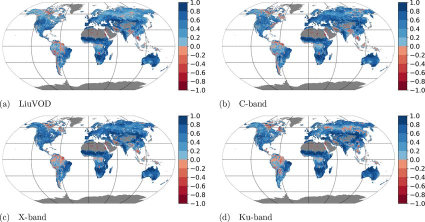
180                                                    L. Moesinger et al.: Vegetation Optical Depth Climate Archive (VODCA)

Table 1. The input VOD data sets used with their temporal coverage, local ascending equatorial crossing times (AECT), and used frequencies
(GHz) for each product.

          Sensor       Time period used        AECT                C-band      X-band    Ku-band    Reference
          AMSR-E       Jun 2002–Oct 2011       13:30                   6.93     10.65       18.70   van der Schalie et al. (2017)
          AMSR2        Jul 2012–Jan 2019       13:30             6.93, 7.30     10.65       18.70   van der Schalie et al. (2017)
          SSM/I F08    Jul 1987–Dec 1991       18:15                                        19.35   Owe et al. (2008)
          SSM/I F11    Dec 1991–May 1995       17:00–18:15                                  19.35   Owe et al. (2008)
          SSM/I F13    May 1995–Apr 2009       17:45–18:40                                  19.35   Owe et al. (2008)
          TMI          Dec 1997–Apr 2015       Asynchronous                     10.65       19.35   Owe et al. (2008)
          WindSat      Feb 2003–Jul 2012       18:00                  6.80      10.70       18.70   Owe et al. (2008)

25 km × 38 km, and 16 km × 27 km. Due to some periods of               2.2.3    AVHRR Vegetation Continuous Fields
non-operation, WindSat contains temporal data gaps (Gaiser
et al., 2004). Unfortunately we were unable to gain access to          We use the Vegetation Continuous Fields (VCF) version 1
data past July 2012, even though WindSat is still operational.         derived from data of Advanced Very High Resolution Ra-
                                                                       diometer (AVHRR) instruments (Hansen and Song, 2018;
                                                                       Song et al., 2018). The VCF product shows the fractional
2.2     Evaluation data                                                cover of bare ground, short vegetation, and tree canopy,
2.2.1    Vegetation optical depth product from Liu et al.,             where trees are defined as all vegetation taller than 5 m in
         VOD_Liu                                                       height, and short vegetation is defined as vegetation smaller
                                                                       than 5 m. VCFs are provided as yearly files from 1982 to
We compared the VODCA data sets with the previously                    2016, indicating the fractional coverage during the local an-
created multi-sensor, multi-band VOD data set (Liu et al.,             nual peak of growing season. The VCF product is retrievable
2011b, 2015), hereafter called VOD_Liu. VOD_Liu covers                 from the online NASA Earthdata Search at https://search.
the period from January 1993 to December 2012 and is based             earthdata.nasa.gov (last access: 9 January 2020).
on VOD retrieved via LPRM from SSM/I (Ku-band), TMI                       Given the relation of VOD with vegetation height and
(X-band), and AMSR-E (C-/X-band) observations. The val-                biomass (Giardina et al., 2018; Liu et al., 2015), it seems
ues are scaled to AMSR-E and methods are in place to fill              sensible to assume that VOD would increase from areas with
gaps due to frozen ground and to correct for large-scale open          bare ground and short vegetation to areas with high tree
water bodies. We expect that the data that are publicly avail-         cover. Hence, we use the VCF data to calculate the mean
able were subject to some temporal smoothing since the data            VCF from 2002 to 2016 and compare them to the mean of
are mostly gap-free. The smoothing is not described in Liu             the VODCA products from 2002 to 2017 (Sect. 4.1). Further-
et al. (2011b, 2015) and the Supplement.                               more, we calculate the VCF trends from 1987 to 2016 and
                                                                       compare it to the trends in the merged Ku-band VOD over the
2.2.2    MODIS leaf area index                                         same period (Sect. 4.4.2). Song et al. (2018) also calculated
                                                                       VCF trends by first determining whether there is a signifi-
To verify the plausibility of VODCA we compare it to
                                                                       cant trend with a Mann–Kendall test and then calculating the
MODIS leaf area index (LAI), MOD15A2H version 6 (My-
                                                                       slope with a Theil–Sen estimator. Both are non-parametric
neni et al., 2015). LAI is the ratio of one-sided leaf area
                                                                       tests that are robust to outliers, but using different methods
to ground area and is estimated from the solar-reflective
                                                                       to mask for significance and estimate the slope can lead to
MODIS bands using a look-up-table-based approach with a
                                                                       significant slopes that are still very small. To avoid this issue,
back-up algorithm that uses empirical relationships between
                                                                       we also calculate the slope using a Theil–Sen estimator and
NDVI, LAI, and fraction of photosynthetically active radia-
                                                                       use the Theil–Sen estimator to determine a 95 % confidence
tion (FPAR). Field studies with different crop types showed
                                                                       interval for the slope and remove any slopes where the zero
that VOD is closely related to LAI (Sawada et al., 2016),
                                                                       slope is within the confidence interval.
a relationship that has already been used to assess VOD
products derived from active sensors (Vreugdenhil et al.,
2017). The data are available globally since 2002 with an              3      Methods
8 d temporal resolution and are for comparison purposes spa-
tially downsampled from their native resolution of 500 m               For each of the VODCA products, we use almost exactly the
to a quarter-degree grid. The original data are available on           same methodology. Exceptions to this common methodology
https://doi.org/10.5067/MODIS/MOD15A2H.006.                            are described at the end of the respective subsection. Each
                                                                       product is computed without any influence of the others. The
                                                                       main difference between the three products is the time period

Earth Syst. Sci. Data, 12, 177–196, 2020                                                  www.earth-syst-sci-data.net/12/177/2020/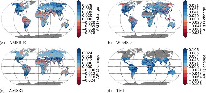
L. Moesinger et al.: Vegetation Optical Depth Climate Archive (VODCA)                                                       181

Figure 1. Time periods of the sensors used for each band.

spanned, resulting from the varying availability of input data         et al., 2009), which is found on all the multi-channel in-
(Fig. 1). The fusion process involves three main processing            struments used in VODCA, and was provided with the
steps: first, preprocessing involves masking for spurious ob-          level 2 VOD data.
servations and spatial and temporal collocation of the data
sets. Second, bias between the different sensors is removed        – Negative VOD values. VOD retrievals < 0 are physi-
by scaling them to AMSR-E VOD. Ultimately, the collocated            cally impossible and are therefore removed from the
and bias-corrected observations of all data sets are merged in       data sets. We also remove VOD values of 0.0 (floating
time and space.                                                      point zero). The reasoning is twofold: first, it is phys-
                                                                     ically only possible to get floating point zero VOD if
3.1   Preprocessing                                                  there is virtually no vegetation, making it very unlikely
                                                                     for most parts of the globe. Second, we also observed
Level 2 VOD data in swath geometry were first projected              that this case occurs surprisingly often in non-desert re-
onto a common regular 0.25◦ × 0.25◦ latitude–longitude grid          gions and that these values never fit well with the other
using nearest-neighbour resampling. The different sensors            observations. This indicates that most VOD values of
visit the same spot on the Earth surface at different times          zero are artefacts that have to be removed.
of the day. To facilitate further processing, we do not take
into account the exact time of observation. Instead, we se-      The above masking is applied independently to all sensors
lected the closest nighttime value in a window of ±12 h for      and bands. A special case is AMSR2, which has two chan-
every UTC midnight which is identical to in the ESA CCI          nels in the C-band, i.e. at 6.9 and 7.3 GHz. If possible, the
soil moisture processor (Dorigo et al., 2017). Since in sub-     observations from the 6.9 GHz band are used, but if the ob-
sequent processing steps the values of different sensors with    servation in this channel is masked, the 7.3 GHz observation
different measurement times will be merged, one can con-         is used instead (if unmasked) to fill gaps. This only causes a
sider the resulting values to be nightly averages.               minor reduction in quality, as the two C-bands are strongly
   Basic masking operations were applied to remove poten-        correlated (Fig. S1). A flag indicating the channel ultimately
tially spurious observations. Specifically we mask for RFI,      used in the merged data set for each observation is provided
low land surface temperatures (LSTs), and VOD values ≤ 0         in the metadata.
as follows.
  – RFI. Artificial microwave emitters on the Earth’s sur-       3.2   Cumulative distribution function (CDF) matching
    face distort the signal received by the satellite, causing
    the resulting VOD values at those locations to be un-        We use a new implementation of the CDF-matching tech-
    reliable. RFI is typically frequency-specific. RFI flags     nique based on a combination of piecewise linear interpo-
    were already provided with the level 2 VOD data and          lation and linear least-squares regression. CDF matching is
    were based on de Nijs et al. (2015). Any observations        used to correct for systematic differences between the VOD
    affected by RFI are removed.                                 values of each sensor, which may result from the individual
                                                                 sensor designs, incidence angles, spatial footprints, and the
  – LST. Due to the different dielectric properties of ice and   slight differences in the frequencies used. The goal of CDF
    water, reliable retrievals can only be made if the ground    matching is to scale a source data set such that its empirical
    is not frozen. Therefore, we remove observations where       CDF becomes similar to the empirical CDF of the reference
    the LST is below 0 ◦ C. Masking for LST was based on         data set. CDF matching is applied on a per-pixel basis and
    the temperature retrievals from the Ka-band (Holmes          has been successfully used for similar tasks that require the

www.earth-syst-sci-data.net/12/177/2020/                                           Earth Syst. Sci. Data, 12, 177–196, 2020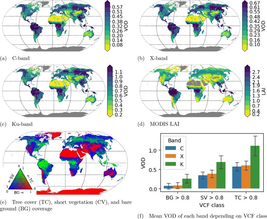
182                                                  L. Moesinger et al.: Vegetation Optical Depth Climate Archive (VODCA)

correction of higher-order differences between data sets (Liu
et al., 2009, 2011a, 2012; Dorigo et al., 2017).

3.2.1   Improvements to ordinary piecewise linear CDF
        matching

Ordinary piecewise linear CDF matching (Liu et al., 2009,
2011a; Dorigo et al., 2017) predicts for each [0, 5, 10, 20,
30, . . . , 80, 90, 95, 100] percentile of the source data the
same percentile of the reference data set. Values between the
nth and nth + 1 percentile are then scaled using linear inter-
polation. While the scaling parameters are determined only
                                                                   Figure 2. Variance of the derived slope, depending on the num-
from temporally overlapping observations, during prediction        ber of observations and the percentile bin for both piecewise linear
there can be values outside the training range. These values       CDF-matching techniques. The colour is log-normalized.
are scaled by extrapolating the first or last percentile inter-
val. This method preserves the ranks of the source and com-
putes rather fast. However, the first and last percentiles are     parameters. For each evenly spaced percentile bin, we deter-
defined by the lowest and highest observations respectively        mine the slope in radians. This is repeated a few thousand
in both source and reference time series. Hence, a single out-     times for various numbers of values (representing time series
lier can greatly affect the parameters of these percentiles,       with a varying number of observations), each time drawing
making them unreliable. Here we propose improvements to            new values. If a CDF-matching method is robust, the deter-
this method to derive more robust scaling parameters that are      mined slopes should have low variance due to the values al-
not specific to VOD data but rather should be generally ap-        ways being drawn from the same distribution.
plicable in similar situations.                                       We run this with both piecewise linear CDF matching and
   The first improvement is to fit a linear model using the        our new method. However, for this simulation we do not dy-
sorted observations smaller than the second percentile with        namically decrease the number of bins, as we are solely in-
an intercept through the second percentile. This gives more        terested in the performance of the linear regression scaling
reliable scaling parameters for low values since all the data      the first and last percentiles. Both methods are tested with
between the lowest and second-lowest percentiles are used          the same randomly drawn data.
instead of just the lowest value. In case a different number          The resulting variances in the slope, for each percentile
of observations exists in the source and reference, the data       bin, for both methods, depend on the number of observa-
with fewer observations are padded by linear interpolation         tions used for the parameter determination. This is shown in
during training. In a similar fashion, a model is fitted for ob-   Fig. 2. The results in the middle bins are exactly the same,
servations above the penultimate percentile. We further in-        as the same methodology is used for these bins. However, in
crease the robustness of the CDF-matching parameters by            the case of linear piecewise interpolation, the slope param-
dynamically increasing the step size of the percentiles if only    eters of the first and last bins have a much higher variance
a few observations are available. The number of observations       than the middle bins as they are affected by outliers. In con-
varies greatly from grid point to grid point and from sensor       trast, the slopes determined by the least-squares method have
to sensor. If too few observations exist between two subse-        a much lower variance. In both cases we can also see that
quent matching percentiles (a “bin”), the CDF matching may         the more observations we have, the lower the variance of the
overfit, leading to unreliable parameters. To counteract this,     slope parameter is, showcasing the reasoning behind reduc-
we dynamically reduce the number of bins and increase the          ing the number of bins dynamically if too few observations
size of the bins based on the number of observations.              are available.

3.2.2   Stability of parameters                                    3.2.3   Practical implementation
To evaluate whether the new matching technique is more ro-         While there is no “true” reference to scale to, AMSR-E has
bust to outliers than the original piecewise linear CDF match-     almost global coverage and has a long temporal overlap with
ing method, we simulate the variances of the derived parame-       all other sensors but AMSR2. Hence, the empirical CDFs of
ters of each bin for a varying number of training observations     WindSat, TMI, and SSM/I are directly scaled to the one of
using artificial values. The use of artificial values allows us    AMSR-E, similar to Dorigo et al. (2015). To preserve any
to test the method without being influenced by the artefacts       potential trends in both source and reference data, only dates
inherent to real data. To achieve this, we sample a set of         when both have a valid observation are used. If at a certain
source and reference values from a standard normal distri-         location fewer than 20 temporal overlapping observations ex-
bution, and then we determine the resulting CDF-matching           ist, no reliable scaling parameters can be determined and the

Earth Syst. Sci. Data, 12, 177–196, 2020                                             www.earth-syst-sci-data.net/12/177/2020/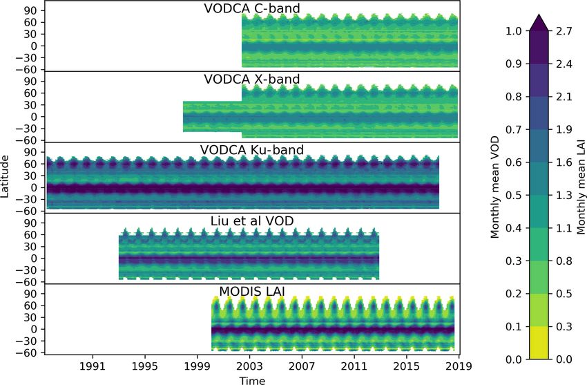
L. Moesinger et al.: Vegetation Optical Depth Climate Archive (VODCA)                                                           183

source time series is dropped. A bin size of 20 was chosen
as a compromise between data coverage and often-used bin
sizes. A bin size of 50 observations is often used as a rule
of thumb for univariate regression to get robust estimates
(Green, 1991). However, our main goal was rather to prevent
time series with very few observations from learning spuri-
ous scaling parameters and we also did not want to lose all
time series with fewer than 50 values. As such 20 was chosen
as a compromise.
   AMSR2 does not share any temporal overlap with AMSR-
E and therefore cannot be directly scaled based on overlap-
ping observations. Instead, for the X- and Ku-bands, scaled
observations of TMI can potentially be used to bridge this
gap. This is done according to the following logic: if possi-
ble, AMSR2 is scaled to the rescaled TMI. Should there not
be enough overlapping observations, the scaling parameters
are determined from all observations of the first 2 years of
AMSR2 and the last 2 years of AMSR-E. While this removes
any potential trends in the first 2 years of the AMSR2 period,
these trends are still assumed to be smaller than the removed
bias. Last, if there are also not enough AMSR2 or AMSR-
E observations available in those years, the whole AMSR2
time series is dropped. For the C-band, which is not cov-
ered by TMI, the AMSR2 data are always matched directly
to AMSR-E by using the last and first 2 years of both sensors.
The published data sets contain a flag indicating the match-
ing method, allowing the user to remove the AMSR2 obser-
vations matched directly to AMSR-E if desired.
   Since the scaling parameters are determined using only a       Figure 3. (a–c) Example X-band time series for a grid cell in Aus-
subset of all observations, during prediction there can be val-   tria (15.125◦ E, 48.125◦ N, mostly farmland with about 20 % forest)
ues outside the training range. The regression is therefore not   at different processing steps. Time series of the original VOD data
forced to go through the origin if the predicted values can po-   of all available sensors are shown in (a), the CDF-matched series
tentially be smaller than 0. These values are deemed unreli-      in (b), and the final merged VOD (VODCA) together with MODIS
able and are removed. However, this occurs very rarely, only      LAI in (c). In (c) VOD and LAI are both normalized, and VOD is
a fraction of about 1/106 to 1/108 of values are lost this way.   downsampled by moving average to match the temporal 8 d resolu-
                                                                  tion of LAI. (d) Violin plot showing the effect of CDF matching on
                                                                  the statistical distribution of VOD.
3.3   Merging
For all bands, the CDF-matched time series of all individual
                                                                  have been proposed to merge multiple satellite observations
sensors are merged into a single long continuous time series.
                                                                  (Gruber et al., 2017, 2019), estimating these weights, i.e. in-
For a certain pixel at a certain time step, three possible sce-
                                                                  dicators of the relative quality of the individual data sets, is a
narios can occur:
                                                                  non-trivial task. This particularly applies to VOD, for which
 1. If on a certain date no sensor has an observation, a data     no appropriate independent reference data exist. However, in
    gap will result in the final product.                         most cases, the arithmetic mean appears to be a robust ap-
                                                                  proximation of optimal merging (Liu et al., 2012).
 2. If only one sensor has an observation, the CDF-matched           Alternatively, one could also take the median instead of the
    value will be directly integrated in the final product.       mean. This would likely be more robust to outliers but would
 3. If multiple sensors have an observation on a certain date,    only make a difference if three or more concurrent values
    their arithmetic mean is taken.                               exist. As such the difference would likely be very small and
                                                                  thus this is not explored in detail.
  This means that the number of sensors contributing to
each observation within a time series can vary greatly. For
each observation in the final product there is a flag indicat-
ing which sensors have contributed to it. Although more so-
phisticated weighted merging methods based on least squares

www.earth-syst-sci-data.net/12/177/2020/                                             Earth Syst. Sci. Data, 12, 177–196, 2020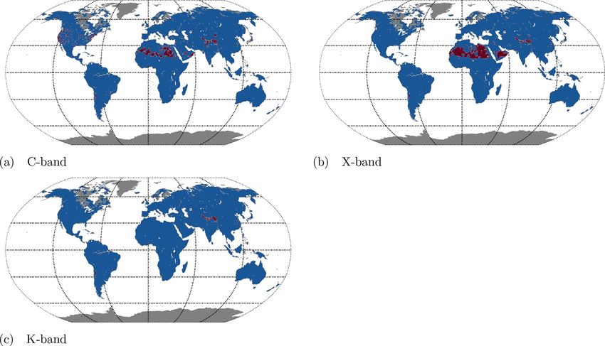
184                                                    L. Moesinger et al.: Vegetation Optical Depth Climate Archive (VODCA)

Figure 4. Global spatial patterns of average multi-sensor VOD from each band (2002–2017), average MODIS LAI (2002–2017), and average
VCF (2002–2016) and distribution of VOD for locations with high tree cover (TC), short vegetation (SV), and bare ground (BG) greater than
0.8. The error bars indicate the standard deviation within each group.

4     Properties of the long-term vegetation optical                   temporally overlapping observations. The merged VOD time
      depth data sets                                                  series shows comparable seasonal dynamics like LAI.
                                                                          The global spatial patterns of average VOD between
4.1    Spatial patterns and temporal dynamics                          June 2002 and June 2017 are shown for each band in Fig. 4a–
                                                                       c. This period was selected because all bands have global
Figure 3 shows an example of X-band VOD time series in                 coverage in this time period. All bands show similar spa-
Austria at different stages of merging procedure together              tial patterns, matching the ones of the VCF land covers
with MODIS LAI. The original VOD time series have vis-                 (Fig. 4e), with high VOD in tropical and northern forests and
ible systematic differences between each sensor. The CDF-              lower VOD in grassland and desert regions. The same pat-
matched VOD time series have been scaled to AMSR-E and                 tern is also visible in canopy height (Simard et al., 2011) and
visually do not show systematic differences between sensors.           MODIS LAI (Fig. 4d), even though the LAI in the tropical
The statistical distributions of VOD from the sensors are sim-         forests is much higher than in the boreal forests, while VOD
ilar after matching (Fig. 3b). This example grid point is north        is similarly high in both regions.
of 38◦ N and thus outside the spatial coverage of TMI; there-             Based on the principle that the penetration of microwaves
fore AMSR2 has been scaled to AMSR-E directly using non-               increases with wavelength, the maximum VOD is highest at

Earth Syst. Sci. Data, 12, 177–196, 2020                                                 www.earth-syst-sci-data.net/12/177/2020/
L. Moesinger et al.: Vegetation Optical Depth Climate Archive (VODCA)                                                        185

Figure 5. Hovmöller diagrams showing the monthly mean VOD per latitude for each band of VODCA and VOD_Liu and for LAI.

shorter wavelengths (Ku-band) and smallest at longer wave-       anomalies should represent either natural variability or arte-
lengths (C-band). This can also be seen in Fig. 4f), which       facts due to shifts in available sensors. In the latter case, one
shows the average VOD of each band for locations domi-           would expect global anomalies to be visible due to either bias
nated by high tree cover (vegetation height > 5 m), short veg-   or differing spatial extent.
etation (< 5 m), or bare ground. Similarly to previous find-        Most anomalies are limited in both space and time and
ings based on the L-band (Konings and Gentine, 2017), this       their start or end does not coincide with a change in sensors,
figure also shows that on average VOD is highest in forests      indicating that they are due to natural causes. Anomalies in
and lowest over bare ground.                                     MODIS LAI show patterns similar to VODCA anomalies,
   The temporal dynamics of VOD across different latitudes       showing that surface events manifest in both in a similar way.
shows plausible seasonal patterns of vegetation phenology        The VOD_Liu anomalies are very similar to the VODCA
(Fig. 5). In general, summer months have the highest VOD:        anomalies, the biggest difference being that the texture is less
in the tropics and subtropics due to increased precipitation     coarse due to the temporal smoothing present.
during that time, and in northern–southern regions due to the       To further assess the stability of VODCA, the correlation
increased temperature and consequent vegetation growth and       of VOD with LAI was calculated for different blending peri-
(leaf) biomass gain.                                             ods similar to in Dorigo et al. (2015) (Fig. 7). The blending
   The VOD time series do not show any visible artificial        periods are chosen for each band such that each period corre-
breaks, indicating that the biases have overall been success-    sponds to a different set of input sensors (Fig. 1) and that each
fully removed from the individual sensors before merging.        period is long enough to calculate reliable coefficients. Both
To make potential artificial breaks more visible, we inves-      the correlation between the raw time series and the anoma-
tigated the seasonal anomalies per latitude (Fig. 6). The        lies indicate that the temporal dynamics are consistent over
anomalies are calculated by collecting all the observations      the whole length of the time series.
of a latitude, calculating the monthly mean, subtracting the
multi-year monthly average, and removing any potential lin-
ear trends using ordinary least-squares regression. Hence the

www.earth-syst-sci-data.net/12/177/2020/                                           Earth Syst. Sci. Data, 12, 177–196, 2020
186                                                 L. Moesinger et al.: Vegetation Optical Depth Climate Archive (VODCA)

Figure 6. Hovmöller diagrams showing anomalies of the monthly means per latitude for each band of VODCA and VOD_Liu and for LAI.

4.2   Spatio-temporal coverage                                       In some locations the merged VOD products have fewer
                                                                  observations than in the original products. This data loss can
The temporal and spatial coverage of the merged VOD time
                                                                  be caused by a failure of the merging procedure, in detail
series for each band is shown in Fig. 8. The coverage of the
                                                                  explained in Sect. 3.2.3. Matching failures are always a re-
merged products is defined by the spatial and temporal cov-
                                                                  sult of insufficient AMSR-E data, and hence the data loss
erage of sensors (Fig. 1). For any band in any time span with
                                                                  occurs in similar regions for all sensors of one band. The
at least one sensor, most parts of the globe have an observa-
                                                                  lack of AMSR-E data is in most cases due to either RFI or
tion for at least 40 % of all days, while in any time period
                                                                  low temperatures in mountainous regions. As an example,
with at least two sensors about 70 % of all days have a valid
                                                                  Fig. 9 shows, for all bands, where the CDF matching failed
observation. TMI is the only sensor with a non-polar orbit
                                                                  for WindSat data. The Ku-band is the least affected (Fig. 9c),
of 35◦ N and S, leading to an increased coverage in that re-
                                                                  where only about 2 % of the grid points are lost, mostly in the
gion in the Ku- and X-bands from 1997 to 2015. The latitude
                                                                  Himalayas. In the X-band the matching fails for about 5 % of
affects the coverage in multiple ways: northern regions are
                                                                  the grid points, mostly in large parts of the Sahara (Fig. 9b).
generally more often covered by the polar-orbiting satellites,
                                                                  The C-band is most affected by data loss (10 %), mostly in
but on the other hand frozen grounds and snow cover inhibit
                                                                  some parts of the USA where additional RFI prevents accu-
the retrieval of VOD in winter. The low coverage band near
                                                                  rate retrievals (Fig. 9a) (Njoku et al., 2005).
23◦ N is the result of LPRM not converging on a valid so-
lution in very arid regions due to the extreme soil dielectric
constants in these regions (de Jeu et al., 2014).
                                                                  4.3   Random error characteristics

                                                                  To validate the performance of our merging approach, we
                                                                  evaluate the change in autocorrelation as an indicator for
                                                                  precision. Merging overlapping observations from multiple
                                                                  sensors is supposed to result in data that have a higher pre-
                                                                  cision than the data of any of the individual sensors. But

Earth Syst. Sci. Data, 12, 177–196, 2020                                           www.earth-syst-sci-data.net/12/177/2020/
L. Moesinger et al.: Vegetation Optical Depth Climate Archive (VODCA) 187
Figure 8. Hovmöller diagrams showing the fraction of days per
month with observations for each latitude and month. The number
of observations of a latitude and month are counted and then divided
by the number of days per month and the number of land grid points
at that latitude.
ucts would lead to an increase in autocorrelation that is re-
lated to the temporal resolution rather than to the precision.
Therefore the temporal resolution is kept unchanged by us-
ing only observation dates existing in both the pre-merge and
post-merge data set.
The autocorrelation differences for the X-band are shown
in Fig. 10. The other bands show similar results and are avail-
able in Figs. S4–S6. The autocorrelation of the merged time
series is on average higher than the autocorrelation of the in-
put series, indicating an overall decrease in noise. However,
sometimes the gain in autocorrelation of one sensor mirrors
the loss of the autocorrelation of the other, likely due to the
former sensor being more noisy than the latter, e.g. in Alaska
or east Russia in the X-band of AMSR-E vs. WindSat. This
means that locally sometimes a single sensor has a higher
Figure 7. Correlation between VODCA and MODIS LAI, raw time precision than VODCA. But there are also regions where the
series, and anomalies, for different blending periods. merged VOD autocorrelation is higher than any of the in-
put time series, e.g in Europe or central North America. This
is likely to occur when all sensors have a similar precision,
without a higher-quality external reference data set, assess- meaning that none of them are dragging the precision of the
ing the change in precision is non-trivial. However, we can others down.
assume that there is supposed to be a high degree of tempo- A noteworthy case is TMI where the autocorrelation of the
ral autocorrelation between subsequent observations because merged time series is almost always higher. This could mean
VOD is related to gradual changes in plant water content and that the TMI data are very noisy and are dragging the overall
biomass (Momen et al., 2017; Konings et al., 2016). There- quality of the merged data down. We investigated this possi-
fore we calculated the difference between the first-order tem- bility by experimentally not including TMI in VODCA. This
poral autocorrelation before and after merging. resulted on average in a lower gain in autocorrelation for the
The autocorrelation coefficient is strongly dependent on other data sets, indicating that the TMI data are still posi-
the temporal resolution. As seen in Sect. 4.2, the temporal tively contributing to the precision of the merged products
resolution of VODCA increases if multiple sensors are avail- by reducing the noise of the end product.
able. Therefore directly comparing the autocorrelation coef-
ficients between the individual sensors and the merged prod-
www.earth-syst-sci-data.net/12/177/2020/ Earth Syst. Sci. Data, 12, 177–196, 2020188 L. Moesinger et al.: Vegetation Optical Depth Climate Archive (VODCA) Figure 9. Data loss during CDF matching of different WindSat bands. CDF matching failed for the red grid points and therefore the data of WindSat at that location are dropped. Very similar looking maps exist for the other sensors in Figs. S7–S9. Figure 10. First-order autocorrelation change due to merging of X-band data for each sensor. Earth Syst. Sci. Data, 12, 177–196, 2020 www.earth-syst-sci-data.net/12/177/2020/
L. Moesinger et al.: Vegetation Optical Depth Climate Archive (VODCA) 189
4.4 Comparison of VODCA with LAI, VOD_Liu, and dence interval do not have the same sign or either of them
Vegetation Continuous Fields is zero are regarded as non-significant and are not displayed
in Figs. 13, 15, and 14 . Figure 13a–c show the C-, X-, and
4.4.1 Correlation between vegetation optical depth and
Ku-band VODCA trends from 19 June 2002 to 19 June 2017
LAI
during which all bands have global coverage. The trends are
A direct validation of VODCA is not possible because of the visually very similar in all bands, confirmed by the spatial
lack of appropriate in situ measurements. Hence it is only Spearman correlation coefficients of 0.88 between the C- and
possible to assess dynamics in VOD with dynamics in re- X-band trends, 0.89 between the C- and Ku-bands, and 0.91
lated variables such as LAI or land cover. Globally, LAI and between the X- and Ku-bands, calculated using only loca-
VODCA time series and their seasonal anomalies are pos- tions where both bands have a significant trend. This further
itively correlated over large areas (Fig. 11). For all bands, reinforces that all bands react very similarly to vegetation
the highest correlations with LAI can be found in grassland- changes. The spatial overlap of trends is shown in Fig. 13d,
dominated regions such as in African savannahs, Australia, where each location is classified based on the sum of posi-
and parts of South America. Correlations are usually lower tive and the sum of negative trends. Locations with no signif-
in forested regions and even slightly negative in parts of icant trend in any band are not displayed. The three classes
tropical forests such as in the Amazon. The negative corre- with contradicting trends (1|1, 2|1, 1|2) are rare as together
lations in tropical forests could be caused by drought peri- they make up only 4.2 % of the displayed points. Conversely,
ods where vegetation water content and hence VOD should 48 % of the land points are covered by the four classes with at
decline but LAI possibly increases (Myneni et al., 2007; least two agreeing trend directions without any contradicting
Saleska et al., 2007), although a green-up of the Amazon un- trend (2|0, 3|0, 0|2, 0|3). The agreement in trends between
der drought is highly debated (Samanta et al., 2010, 2012; frequencies indicates that the longer Ku-band series can be
Morton et al., 2014). However, this comparison of VODCA used as an indicator of the shorter X- and C-band series in
and LAI demonstrates that VODCA reflects plausible sea- trend analyses. Further, the LAI trends of the same time pe-
sonal and short-term changes in vegetation and will likely riod (Fig. 13e) match the VOD trends very well overall, even
provide additional information on vegetation dynamics on though in detail the strength and location of the trends vary.
top of LAI and other related optical biophysical vegetation The trends of Ku-band VODCA and VOD_Liu were de-
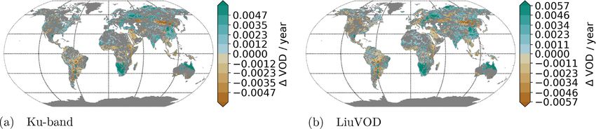
products from optical remote sensing. termined (Fig. 14) to assess whether studies that have been
To assess differences between the temporal dynamics of analysing VOD trends using VOD_Liu would get different
VODCA and VOD_Liu, we compared both to MODIS LAI. results if they were repeated using the VODCA Ku-band
Because VOD_Liu is temporally smoothed, comparing daily instead. The Ku-band VODCA is used because it has the
values is inadequate. Instead, we first resample both data longest overlap with VOD_Liu (1993–2012).
sets to monthly averages and calculate the Spearman corre- On a global scale, we see the almost exact same patterns
lation to the also monthly averaged MODIS LAI, only using in both VOD series; therefore studies performed at that scale
dates existing in all data sets. The downsampling leads to would get similar results for both data sets. However, on a lo-
slightly higher correlation coefficients (Fig. 12) than using cal scale the patterns differ sometimes; e.g. in most of Turkey
the daily values (Fig. 11) due to decreased noise, while the the Ku-band VODCA shows an increase, while VOD_Liu
spatial patterns stay the same. The highest correlation was shows a decrease in VOD. As such regional studies might
the VODCA X-band, with a global average of 0.42, followed get very different results case-by-case depending on which
by the VODCA Ku- and C-bands with 0.39 and 0.37 respec- data set is used.
tively. The lowest on average is VOD_Liu with 0.33. It could Taking advantage of the much longer length of the Ku-
be that the lower correlation is a result of being a mix of mul- band, another trend analysis is done for this band using the
tiple bands or because the VODCA products use more input data from 1987 to 2016 (Fig. 15g) to give a first impression of
data sets, resulting in more accurate values. Either way, this the changes within the last 30 years. Overall we see a decline
indicates that the VODCA products capture temporal dynam- in VOD in the tropics, likely due to deforestation, and in large
ics better. parts of Mongolia, attributed to variations in rainfall and sur-
face temperatures as well as increased livestock farming and
wildfires (Liu et al., 2013). VOD increased strongly in India
4.4.2 Trend analysis of VODCA, VOD_Liu, LAI, and
and large parts of China, mostly due to an increase in crop-
Vegetation Continuous Fields
lands in the former case and due to both an increase in for-
To evaluate the relationship between the C-, X-, Ku-band est and croplands in the latter (Chen et al., 2019). VOD also
VODCA, VOD_Liu, MODIS LAI, and VCF changes and to increased in northern parts of Australia, matching trends in
gain a first insight into the long-term changes in VOD, we FPAR and precipitation seen in Donohue et al. (2009). Other
assess linear trends in the data sets. Yearly averages are used regions with increasing VOD are southern Africa and central
to determine the trends and their confidence intervals via the North America. Of a questionable nature is the widespread
Theil–Sen estimator. Trends whose upper and lower confi- positive trend in the Sahara given LPRMs struggle to re-
www.earth-syst-sci-data.net/12/177/2020/ Earth Syst. Sci. Data, 12, 177–196, 2020190 L. Moesinger et al.: Vegetation Optical Depth Climate Archive (VODCA)
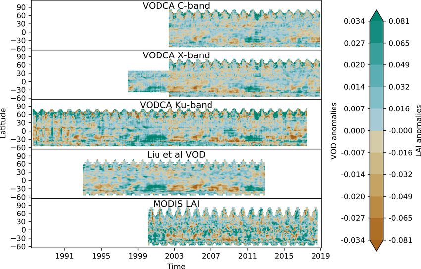
Figure 11. Spearman correlation coefficient between VODCA VOD and MODIS LAI for each band. Panels (a, c, e) show the correlation
for the absolute signal, and (b, d, f) for the anomalies from the long-term VOD climatology.
trieve VOD here. Most of the changes observed for VOD are 5 Current limitations and possible improvements
mirrored in the VCF changes from 1987 to 2016 (Fig. 15f;
see Sect. 2.2.3 for details). The large bare-ground losses in 5.1 AMSR2 scaling to TMI
India, China, and the north African shrubland manifest as
Upon closer inspection of the trends in Fig. 13, we can see a
positive VOD trends. Likewise, the deforestation in South
spatial break in North America in X- and Ku-band trends at
America and land degradation with hotspots in Mongolia,
35◦ N. North of this latitude AMSR2 data of 2012–2014 were
Afghanistan, or the southwestern USA coincide with a loss in
matched to the AMSR-E data of 2010–2012, while south
VOD. Also, the patterns of tree cover gain in eastern Europe
of this line temporally overlapping scaled TMI values were
and European Russia coincide with increased VOD. While
used to bridge the gap between the two sensors. Unusually
there do not seem to be any areas where VOD and VCF con-
low VOD values can be observed in this region in the years
tradict each other clearly, some trends are only visible in one
2012 to 2015 in both the X- and Ku-bands. This indicates
of the data sets. For example the strong increase in VOD in
that the CDF matching does not correct the bias between the
southern Africa cannot be observed in VCF.
sensors but artificially removes the difference that is due to
surface processes. Consequently, the matched AMSR2 data
have a slight positive bias north of 35◦ N in large parts of
North America. For users, we advise to be careful when us-
ing X- and Ku-band values after July 2012 north–south of
Earth Syst. Sci. Data, 12, 177–196, 2020 www.earth-syst-sci-data.net/12/177/2020/L. Moesinger et al.: Vegetation Optical Depth Climate Archive (VODCA) 191
Figure 12. Correlation of monthly VOD_Liu and the VODCA products with MODIS LAI. For this analysis, the data are first resampled to
monthly averages, and then only the months where all four data sets have values are used.
35◦ N and S as well as C-band values after July 2012 glob- very similar characteristics, the VOD signal at each location
ally as the AMSR2 data might induce a bias. Currently there may still have its unique features resulting from land surface
exists a flag indicating how AMSR2 has been CDF-matched. characteristics or vegetation species composition.
With ongoing AMSR-E vs. AMSR2 Level 1 intercalibration
efforts by JAXA we expect to reduce spurious observations 5.3 Data gaps in the input data sets leading to
in the AMSR2 period in the near future. increased noise
Averaging multiple temporally overlapping observations re-
5.2 Data loss while CDF matching duces noise (Sect. 4.3). However, this can only be done if
overlapping observations exist. While theoretically the max-
As described earlier, CDF matching failed because of miss- imum number of observations is defined by the number of
ing AMSR-E data in some regions, mostly in the Himalayas available sensors, in practise usually fewer observations are
(Fig. 9). One possible solution to avoid this data loss would available due to gaps in the individual time series. Hence,
be to substitute the CDF-matching parameters of these lo- filling short gaps in the original time series of each sensor
cations with the parameters from locations with similar dy- could potentially increase the precision of VODCA. Since
namics in VOD. This could be done by clustering the time VOD changes slowly over time (Konings et al., 2016), it is
series and using the parameters of another location within intuitively clear that even if a sensor has no valid observa-
the same cluster. Taking this one step further, one could also tion on a certain date, the value is expected to be similar to
investigate the possibility of using all the data in one clus- the value of the dates before and after. Therefore one could
ter to derive a single set of CDF-matching parameters and fill short gaps with a model that at least implicitly uses au-
use these to scale all the source time series within it. Not tocorrelation for its predictions, such as Gaussian processes
only would this allow us to scale all the data without loss, (Camps-valls et al., 2017).
but the increased number of values available for each pa-
rameter determination would also lead to more robust CDF
5.4 L-band product
parameters. However, generating meaningful clusters from
hundreds of thousands of long time series containing miss- An L-band product would be of great use to the scien-
ing values while keeping the computational cost at bay is tific community, as L-band VOD has been instrumental in
anything but trivial (e.g. Mikalsen et al., 2018). In addition, analysing vegetation patterns (e.g. Brandt et al., 2018a; Tian
even though clusters may be composed of time series with et al., 2018; Brandt et al., 2018b; Chaparro et al., 2018). Al-
www.earth-syst-sci-data.net/12/177/2020/ Earth Syst. Sci. Data, 12, 177–196, 2020192 L. Moesinger et al.: Vegetation Optical Depth Climate Archive (VODCA) Figure 13. Trends of various bands between 2002 and 2017 of VOD (a–c) and LAI (e). Non-significant trends are not displayed; the trends are calculated by Theil–Sen regression using yearly mean values. Panel (d) shows trend classes based on the number of VOD bands exhibiting a positive|negative trend. For example, 2|1 indicates that two VOD bands show a significant positive trend, while one band shows a significant negative trend. Their order and colour are indicative of the likelihood of the trend. Figure 14. Trends between 1993 and 2012 of Ku-band VODCA (a) and VOD_Liu (b). Non-significant trends are not displayed; the trends are calculated by Theil–Sen regression using yearly mean values. though we produced an experimental L-band product based terms of temporal extent nothing is gained. Second, the tem- on LPRM-SMAP and LPRM-SMOS using the same method- poral coverage is highly unbalanced, with the SMAP period ologies as for the other bands, the evaluation of this L-band having a much higher density. This carries the high risk that product showed that it is not yet fit for release for a number of users might apply unfitting methods to the data. Third, the au- reasons. First, merging SMOS and SMAP does not result in a tocorrelation analysis indicated that VODCA-L has a higher time series that is longer than just SMOS alone; therefore in level of noise than pure LPRM-SMAP. Nevertheless, given Earth Syst. Sci. Data, 12, 177–196, 2020 www.earth-syst-sci-data.net/12/177/2020/
You can also read