Modelling landslide hazards under global changes: the case of a Pyrenean valley - Natural Hazards and Earth System Sciences
←
→
Page content transcription
If your browser does not render page correctly, please read the page content below
Nat. Hazards Earth Syst. Sci., 21, 147–169, 2021
https://doi.org/10.5194/nhess-21-147-2021
© Author(s) 2021. This work is distributed under
the Creative Commons Attribution 4.0 License.

Modelling landslide hazards under global changes:
the case of a Pyrenean valley
Séverine Bernardie1 , Rosalie Vandromme1 , Yannick Thiery1 , Thomas Houet2 , Marine Grémont3 , Florian Masson1 ,
Gilles Grandjean1 , and Isabelle Bouroullec4
1 BRGM,  3 avenue Claude Guillemin, 45060 Orléans, France
2 LETG-Rennes  UMR 6554 CNRS, Place du Recteur Henri Le Moal, 35043 Rennes CEDEX, France
3 SUEZ, 34078 Montpellier, France
4 BRGM, 31520 Ramonville-Saint-Agne, France

Correspondence: Séverine Bernardie (s.bernardie@brgm.fr)

Received: 20 September 2019 – Discussion started: 30 January 2020
Revised: 25 August 2020 – Accepted: 10 October 2020 – Published: 18 January 2021

Abstract. Several studies have shown that global changes             Therefore, even if future forest growth leads to slope sta-
have important impacts in mountainous areas, since they af-          bilization, the evolution of the groundwater conditions will
fect natural hazards induced by hydrometeorological events           lead to destabilization. The increasing rate of areas prone to
such as landslides. The present study evaluates, through an          landslides is higher for the shallow landslide type than for
innovative method, the influence of both vegetation cover            the deep landslide type. Interestingly, the evolution of ex-
and climate change on landslide hazards in a Pyrenean valley         treme events is related to the frequency of the highest water
from the present to 2100.                                            filling ratio. The results indicate that the occurrences of land-
   We first focused on assessing future land use and land            slide hazards in the near future (2021–2050 period, scenario
cover changes through the construction of four prospective           RCP8.5) and far future (2071–2100 period, scenario RCP8.5)
socioeconomic scenarios and their projection to 2040 and             are expected to increase by factors of 1.5 and 4, respectively.
2100. Secondly, climate change parameters were used to ex-
tract the water saturation of the uppermost layers, according
to two greenhouse gas emission scenarios. The impacts of
land cover and climate change based on these scenarios were          1   Introduction
then used to modulate the hydromechanical model to com-
pute the factor of safety (FoS) and the hazard levels over the       Global changes have impacts worldwide, but their effects
considered area.                                                     are even more exacerbated in particularly vulnerable areas,
   The results demonstrate the influence of land cover on            such as mountainous regions. In these areas, a range of so-
slope stability through the presence and type of forest. The         cioeconomic sectors (e.g. tourism, forest production, agro-
resulting changes are statistically significant but small and        pastoralism and natural resources) have experienced consid-
dependent on future land cover linked to the socioeconomic           erable changes in the last 2 centuries, resulting in pressures
scenarios. In particular, a reduction in human activity results      on natural resources and traditions that are imposed by in-
in an increase in slope stability; in contrast, an increase in an-   creasingly industrialized societies (Huber et al., 2005). Some
thropic activity leads to an opposite evolution in the region,       mountainous regions have been extensively transformed,
with some reduction in slope stability.                              converting them from inaccessible and relatively poor areas
   Climate change may also have a significant impact in some         into attractive destinations for the wealthy. In other cases,
areas because of the increase in the soil water content; the         outmigration and an ageing population have led to economic
results indicate a reduction in the FoS in a large part of           declines in the agro-pastoral and forestry sectors.
the study area, depending on the landslide type considered.             Climate change affected and will affect mountainous re-
                                                                     gions. An increase in the temperature in these areas has al-

Published by Copernicus Publications on behalf of the European Geosciences Union.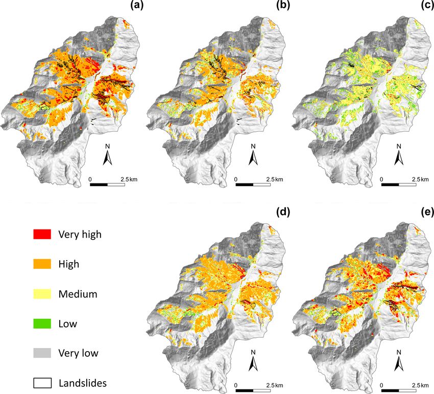
148                                                   S. Bernardie et al.: Modelling landslide hazards under global changes

ready been observed that is comparable to what has been ob-       al., 2018) and also in their seasonal temporality (Stoffel et
served in lowland regions (Kohler and Maselli, 2009). Some        al., 2014); these factors will evolve differently depending on
boundaries, such as the tree line, the limit of snow and the      the region of interest.
limit indicating the presence of glaciers and permafrost, start       Landslide hazards may also be affected by global change
to be modified. The hypothesis of global warming has now          with the evolution of the socioeconomic contexts, which may
been validated by various studies (IPCC, 2007, 2014). The         have some impacts on landslides through the evolution of
climate evolution have significant impacts of natural haz-        land cover, as demonstrated in several studies (Vanacker et
ards since most of them are induced by hydrometeorologi-          al., 2003; Van Beek and Van Ash, 2004; Promper et al., 2014;
cal events, such as floods and different types of landslide.      Reichenbach et al., 2014; Galve et al., 2015; Persichillo et
For example, the IPCC (Intergovernmental Panel on Climate         al., 2017; Pisano et al., 2017; Gariano et al., 2018). In par-
Change) notes that “There is high confidence that changes         ticular, the abandonment of agricultural practice and land
in heatwaves, glacial retreat, and/or permafrost degradation      management result in an increasing number of shallow land-
will affect slope instabilities in high mountains, and medium     slides (Persichillo et al., 2017; Pisano et al., 2017; Gariano et
confidence that temperature-related changes will influence        al., 2018).
bedrock stability. There is also high confidence that changes         Indeed, vegetation influences deep-seated landslides very
in heavy precipitation will affect landslides in some re-         little, but this influence exists for shallow landslides and re-
gions” (IPCC, 2014). In the Pyrenees, an OPCC-CTP re-             mains difficult to address. At the same time, the vegetation
port (2018) mentioned that “It is highly probable that the        cover increases the ground weight and thus tends to initiate
Pyrenees will see an increase in extreme weather phenom-          ruptures, but it also increases the shear strength and modi-
ena”. This may lead to more frequent floods, landslides,          fies the soil moisture content through evapotranspiration and
rockfalls and avalanches. Nevertheless, the quantification of     runoff processes. The relative importance of these two con-
the impacts of climate change on natural hazards related to       trary effects varies according to the localization of the vege-
hydro-geohazards remains a complex issue. Among hydro-            tation cover on the slope. The stability is increased if the veg-
geohazards, landslides are very sensitive to the hydrometeo-      etation is present on the toe of the slope (Genet et al., 2010;
rological conditions present in mountainous regions and are       Ji et al., 2012), but this stabilizing effect is reduced if the
complex. Gariano and Guzzetti (2016) indicate that several        vegetation is located on the upper part of the slope (Norris,
landslide-triggering parameters may be affected by climate        2008; Genet et al., 2010). As a result, the densification of
change. Indeed, climate change occurring in mountains may         forest areas may improve the slope stability (Reichenbach et
imply future modifications in temperature and precipitation       al., 2014).
patterns; this may lead to changes in the balance between             Many studies have been conducted based on historical ob-
snow, ice and rainfall, which ultimately will result in changes   servations; these analyses, which use empirical or numerical
in precipitation quantity and seasonality. Landslides are also    approaches, permit the analysis of the evolution of differ-
sensitive to the presence of water within the layers that are     ent features of landslides (frequency, type, evolution of the
susceptible to movement. As future trends in the climate may      mechanisms, etc.). The quantification of future scenarios is
imply some modifications of meteorological parameters such        a key challenge in estimating the future trends in landslide
as precipitation and temperature, the resulting underground       activity with the future evolution of climate change, and es-
water table level may evolve.                                     timating the uncertainties is necessary in these approaches.
   The sensitivity of landslides to climate change may de-        For this reason, modelling constitutes an approach that is be-
pend on their type, especially on the size and depth of the       ing increasingly developed in two different ways, depend-
landslide (Crozier, 2010). As shallow landslides are gener-       ing on the size of the investigated area: (a) physical mod-
ally governed by shorter-duration rainfall, they may be more      els and (b) statistical models. The majority of physical ap-
influenced by the evolution of parameters in the short-term       proaches are local and investigate a portion of a slope, a sin-
parameter evolution, such as changes in the intensity of rain-    gle slope or a single landslide (Buma and Dehn, 1998, 2000;
fall. In contrast, deep-seated landslides may be affected by      Dehn and Buma, 1999; Tacher and Bonnard, 2007; Bonnard
long-term hydrometeorological evolutions, such as changes         et al., 2008; Comegna et al., 2013; Rianna et al., 2014; Vil-
in the monthly rainfall, seasonal snow or groundwater. Sev-       lani et al., 2015; Collison et al., 2000; Chang and Chiang,
eral studies are related to the analysis of the impact of cli-    2011; Coe, 2012; Melchiorre and Frattini, 2012). In con-
mate change on landslide occurrence. The review conducted         trast, many studies based on statistical approaches analyse
on that topic, described in Gariano and Guzzetti (2016), indi-    future climate change impacts on landslides at regional scales
cates the increasing number of studies devoted to this issue.     (Jakob and Lambert, 2009; Jomeli et al., 2009; Turkington et
The future evolution of hydrometeorological conditions im-        al., 2016; Lee et al., 2014; Winter and Shearer, 2015; Cia-
plies that there will be some modification in the frequency       batta et al., 2016; Fan et al., 2013; Kim et al., 2015; Gassner
of landslide occurrence (Turkington et al., 2016; Gariano et      et al., 2015; Shou and Yang, 2015; Wu et al., 2015; Gariano
al., 2017; Rianna et al., 2017; Robinson et al., 2017; Alvi-      et al., 2017; Sangelantoni et al., 2018).
oli et al., 2018; Peres and Cancelliere, 2018; Sangelantoni et

Nat. Hazards Earth Syst. Sci., 21, 147–169, 2021                                   https://doi.org/10.5194/nhess-21-147-2021
S. Bernardie et al.: Modelling landslide hazards under global changes                                                              149

   The performance of statistical models versus physical                    pathways, according to the standards defined by the
models has been compared in several studies (e.g. Cervi                     IPCC) RCP4.5 and RCP8.5.
et al., 2010; Zizioli et al., 2013; Davis and Blesius, 2015;             The impacts of land cover and climate change are then ad-
Ciurleo et al., 2017; Bartelletti et al., 2017; Galve et al., 2017;   dressed through these different scenarios that provide the fu-
Oliveira et al., 2017). Some results indicate slightly bet-           ture evolution of hydromechanical parameter variations used
ter results with deterministic models (Ciurleo et al., 2017),         to compute the hazard levels. The hydromechanical model
whereas some others demonstrate the better performance of             is based on a large-scale slope stability assessment tool that
statistical ones (Galve et al., 2017; Bartelletti et al., 2017).      combines a mechanical stability model, a vegetation module
These variations can depend on the assumptions made on                that modulates the stability parameters to take into account
hydrogeological system model and on the knowledge of the              the effects of vegetation on the mechanical soil conditions
input parameters.                                                     (cohesion and overload) and a hydrogeological model that
   The advantages of physical models, in the case of accu-            provides the water table level computed from meteorologi-
rate characterization of the sites, are the quantification of the     cal temporal data. The main algorithm computes a spatially
effect of future climate scenarios on landslides at a regional        distributed factor of safety (FoS) for the two selected future
scale, permitting the consideration of the spatial variability of     periods (2040 and 2100) and the different LUCC models.
the environmental parameters, and the quantification of the
evolution of the hazard. However, it appears that there are           2.1   ALICE slope stability model
still few studies dedicated to the quantification of the impact
of future climatic and land cover scenarios on landslides.            ALICE (Assessment of Landslides Induced by Climatic
   In this study, the impacts of global change on landslide           Events) was developed by the French Geological Survey
hazards is analysed according to two features: (i) the evolu-         (BRGM) to support landslide susceptibility assessment and
tion of land cover, which can be analysed as the evolution of         mapping for areas ranging from individual slopes to re-
vegetation cover and its effects on landslides, and (ii) the evo-     gions (Sedan et al., 2013; Baills et al., 2011; Vandromme
lution of climatic conditions, which result in the evolution of       et al., 2015; Thiery et al., 2017; Vandromme et al., 2020).
the hydrogeological conditions. Different types of landslides         Developed in a GIS (geographic information system) envi-
are considered here, and the effects of global changes on each        ronment, it is a physically distributed model based on a limit
of them are analysed. This analysis is conducted within a             equilibrium method that computes FoS along 2D profiles
Pyrenean valley in a high-elevation context. We first intro-          over the entire area. It can integrate different landslide ge-
duce an overview of the method for evaluating the impact              ometries, the spatial and inherent heterogeneity of the surfi-
of global change on landslide hazards. Then, the mechanical           cial deposits and geology and their geotechnical parameters,
and hydrogeological models are briefly presented, as well as          triggering factors (i.e. water and seismicity), and land cover
the geological setting of the studied site. The socioeconomic         change. The 3D geometry of the studied area is entered as
and climatic scenarios and the way they are used in the me-           a dataset in raster format: topography and layer interfaces
chanical and hydrogeological models are described. The last           are represented with different DEMs (digital elevation mod-
section presents the results of the modelled scenarios and a          els). Geomechanical characteristics, namely, cohesion (c0 ),
final discussion of the results.                                      friction angle (φ 0 ) and volumetric weight (γ 0 ), are associated
                                                                      with each geologic and surficial-deposit layer. These param-
                                                                      eters can be implemented with a constant value or with prob-
2   Modelling method                                                  abilistic distributions to take into account the environmental
                                                                      variability of these parameters and the uncertainties associ-
The evaluation of the impacts of global change on landslide
                                                                      ated with the values of these parameters. Like the other ge-
activities is realized through the analysis of the effects of
                                                                      ometrical inputs of the model, the ground water table level
both vegetation cover and meteorological conditions on land-
                                                                      (GWL) is implemented in raster format, as a piezometric
slide activities; this analysis was conducted with the follow-
                                                                      map: a minimum level and a maximum level are required.
ing method (Bernardie et al., 2017; Grandjean et al., 2018):
                                                                      Then, the GWL can be implemented empirically between a
    - The assessment of future land cover is addressed                saturation level from 0 (dry conditions, minimum level) to
      through the construction of four prospective socioeco-          1 (saturated conditions, maximum ground water level). The
      nomic scenarios and their projection to 2040 and 2100,          2D profiles are automatically generated from a digital eleva-
      which are then spatially modelled with land use and             tion model using the local drain direction. A slope stability
      land cover change (LUCC) models.                                assessment is performed on each 2D profile, and each profile
                                                                      covers the whole studied area. The slope stability calculation
    - The climate change inputs for this study correspond to          is performed considering the forces applied on sliding bod-
      two greenhouse gas emissions scenarios. The simula-             ies along a potential slip surface that can be circular or along
      tions were performed with the greenhouse gas (GHG)              an interface. The rotational slip surfaces are characterized by
      emissions scenarios (RCP: representative concentration          length, a minimal depth and a maximal depth. The shallow

https://doi.org/10.5194/nhess-21-147-2021                                       Nat. Hazards Earth Syst. Sci., 21, 147–169, 2021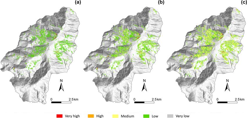
150                                                    S. Bernardie et al.: Modelling landslide hazards under global changes

translational slip surfaces are defined by an interface, a length      This method results in an analysis of the dynamic evolu-
and a scarp angle. The shear strength of the soil along the         tion of landslide susceptibility in the area of interest. Land-
potential failure plane is given by the Mohr–Coulomb failure        slide hazard assessment considers runout, the magnitude and
criterion. The Morgenstern and Price (1965, 1967) method            the return period for a given intensity (Varnes, 1984). As in
is used to calculate FoS. Once all parameters (geometrical,         many cases, the hazard analysis is not completed. Notably,
geotechnical, landslide type and triggering factor) are imple-      runout is not accounted for in this study. Nevertheless, the
mented in the model, several sliding surfaces are computed          landslide susceptibility assessment is converted into land-
along each profile. The sliding surface with the lower FoS is       slide hazard assessment by expert knowledge (Van Western
kept, and this value is attributed to every cell concerned by       et al., 2006, 2008; Corominas et al., 2014).
this sliding surface. Moreover, in the objective of improving
the accuracy of the calibration and the validation, a strategy      2.4    Validation of the model
for calibrating all the parameters has been developed (Van-
dromme et al., 2020).                                               Because this study is focused on the probability of slope fail-
                                                                    ure (i.e. initiation), the boundaries of active landslides are
2.2   GARDÉNIA hydrological model                                   classified into two zones: (i) the zone of depletion and (ii) the
                                                                    zone of accumulation (Varnes, 1978).
The hydrogeological model GARDÉNIA (modèle Global                      From the zone of depletion, and the very high and high
À Réservoirs pour la simulation de DÉbits et de NIveaux             hazard classes defined from the FoS values, several statistical
Aquifères; Thiéry, 2003) is a lumped hydrological model.            tests can be computed: the relative error (ξ ), receiving oper-
It simulates the main water cycle mechanisms in a catch-            ating characteristic curve and associated area under the curve
ment basin (rainfall, snowmelt, evapotranspiration, infiltra-       (ROC (AUC)), prediction rate (PR (AUC)), true positive rate
tion and runoff) by applying simplified laws of physics to          (TPr), and false positive rate (FPr). These classical evalu-
flows through successive reservoirs. It considers a system of       ation and validation tests are defined by Brenning (2005),
three tanks, reproducing the three-layer characteristics of the     Beguería (2006), Guzzetti et al. (2006), and Vandromme et
hydrological behaviour of the soil: (i) the top zone, i.e. the      al. (2020). They allow for the assessment of the predictive
first 10 cm, where evapotranspiration occurs; (ii) the unsatu-      power of the simulated maps (Brenning, 2005). ξ measures
rated zone, where runoff occurs; and (iii) the saturated zone.      the model performance; it is defined as the total proportion
Once calibrated, the model permits us to (i) calculate the bal-     of observations (i.e. the zones of depletion) correctly clas-
ance of rainfall, snowmelt, evapotranspiration, runoff and in-      sified in the very high and high hazard classes (Thiery et
filtration into the underlying aquifer; (ii) analyse the consis-    al., 2007). ROC (AUC) indicates the degree to which the
tency between meteorological observations and observations          zones of depletion are explained by the computed FoS. It
of flow rates or piezometric levels; (iii) recreate, for a given    is a tool for validating the different models by a threshold-
catchment basin, the flow rates of a river or spring and/or the     independent measure of discrimination between the propor-
piezometric levels at a given point in the aquifer during peri-     tion of correctly predicted positive cases and the proportion
ods when measurements are not available; and (iv) simulate          of correctly predicted negative cases (Brenning, 2005). The
flow rates resulting from dry periods or unusual precipitation      values fluctuate between 0.5 (no discrimination) and 1 (per-
sequences, groundwater piezometric levels, observed precip-         fect discrimination). The PR (AUC) is computed on the ba-
itation and precipitation resulting from scenarios (drought or      sis of the different FoS values and the zones of depletion.
high-water periods resulting from climate change scenarios).        It is obtained by varying the decision threshold and plotting
For our purpose, it allows for the estimation of the daily lo-      the respective sensitivities against the total proportions of the
cal piezometric level evolution based on the meteorological         zones of depletion. It provides a validation index of the sim-
parameters that might evolve due to climate change.                 ulated maps (Chung and Fabbri, 2003). Finally, TPr and FPr
                                                                    are the proportion of correctly classified observations and the
2.3   Linking slope stability and hydrological models               proportion of incorrectly classified observations, respectively
                                                                    (Thiery et al., 2007; Vandromme et al., 2020).
The spatialized piezometric level can then be integrated into
the slope stability assessment equations developed in AL-
ICE. In this approach, a significant approximation is made          3     The Cauterets basin, its geological setting and
by spatializing the piezometric level in the surficial forma-             available data
tions; the ground reality is much more complex. This so-
called piezometric level has to be considered an indicator of       The Cauterets municipality is representative of the climatic,
the water content of the soil, which will promote slope desta-      lithological, geomorphological and land cover conditions ob-
bilization. This indicator is called the “water filling ratio”: a   served in the French Central Pyrenees (Viers, 1987). The mu-
value of one means that the water table level is at its maxi-       nicipalities are highly affected by several natural hazards,
mum, and zero means that the level is at its minimum.               such as landslides, rockfalls, debris flows and flash floods,

Nat. Hazards Earth Syst. Sci., 21, 147–169, 2021                                     https://doi.org/10.5194/nhess-21-147-2021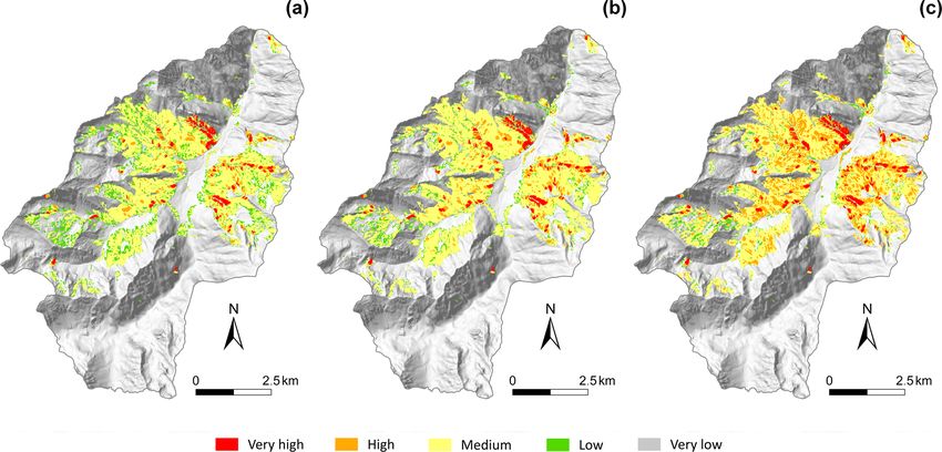
S. Bernardie et al.: Modelling landslide hazards under global changes                                                           151

and the area was restored by Restauration des Terrains de           to respect the modelling capabilities of ALICE, only land-
Montagne Survey (RTM) from the National Forests Office              slides with translational and rotational shear surfaces (ac-
(ONF) at the end of the 19th century (De Crécy, 1988). Dom-         cording to the classification from Cruden and Varnes, 1996)
inated by ridgelines, with a maximum elevation of approxi-          were selected in the inventory. Figure 1 and Table 1 depict the
mately 2500 m a.s.l., the municipality is subject to oceanic        morphology and morphometric–environmental characteris-
climatic influences, with an average rainfall of 1157 mm yr−1       tics of the different landslide types that have high confidence
and a thermal amplitude of 13 ◦ C, typical for a mountain           index values.
area (Gruber, 1991). However, under the oceanic influence,             We will consider the following four types (one transla-
the valley is marked by a mountainous climate with intense          tional and three rotational): (i) shallow translational land-
storms during summer and autumn and large snowfalls dur-            slides, which occur mainly in various colluviums and weath-
ing winter (it is often the snowiest resort area in France). This   ered materials (especially in weathered schist) from gentle
enclosed valley juxtaposes several types of fractured lithol-       to very steep slopes (from 12 to 47◦ ); (ii) shallow rotational
ogy and reliefs with different exposures and strong eleva-          landslides, which occur in thin moraine deposits (colluviums,
tion variations (Barrère et al., 1980). Consequently, the open      removed-moraine deposits or moraines in place) from mod-
slopes located above 1600 m a.s.l. with eastern exposure have       erately to very steep slopes (from 17 to 50◦ ), the majority of
more sunshine in summer and more snowfall in winter than            which are located near streams and are triggered by a basal
the valley bottom or the slopes exposed to the west.                incision caused by torrents; (iii) moderately deep rotational
   The test site is located in the middle part of the munici-       landslides; and (iv) deep rotational landslides, which have a
pality of Cauterets in an area of approximately 70 km2 and is       common rotational shear surface in the initiation zone. These
characterized by a large variety of landslides. It can be sub-      occur in materials such as moraine deposits and/or weathered
divided into three geomorphological units. The southern unit        materials at deeper depths. They are located on gentler slopes
is dominated by plutonic magmatic rocks (especially gran-           than shallow landslides (from 11 to 35◦ ).
ites) overlapped by limestones, while the western and eastern          Table 2 outlines the main predisposing factors affecting
units are composed of metamorphic rocks (especially schists         each landslide type. The different thematic data are derived
and sandstone) with intercalation of limestone. The lithol-         from (i) air-photo interpretation analysis, (ii) airborne lidar
ogy can be overlapped by morainic deposits on gentle slopes         surveys, (iii) satellite imagery analyses and (iv) field surveys.
and morainic colluviums on the steepest slopes (Barrère et          The DTM (10 m resolution) is derived from the airborne li-
al., 1980; Viers, 1987).                                            dar data. The slope gradient map and the flow accumula-
   A landslide inventory was compiled at a 1 : 10 000 scale         tion map are derived from the DTM. The lithological map is
through a diachronic interpretation of several data sources         based on the main lithological units described in a geological
(i.e. air-photo interpretation between 1950 and 2016, ortho-        map produced by the French Geological Survey (Barrère et
image analysis, landform analysis with an accurate DTM              al., 1980) at a 1 : 50 000 scale and is completed by fieldwork.
(digital terrain model) analysis and interpolation of triplets      The surficial-formation map is obtained by a geomorphologi-
obtained by lidar in 2016, literature analysis) completed by        cal approach with the segmentation of homogeneous areas of
field surveys. A total of 346 objects were identified, in-          the landscape associating surficial-formation type, their fa-
cluding landslides with rotational shear surfaces, landslides       cies and the processes following the approach developed by
with translational shear surfaces and deep-seated gravita-          Thiery et al. (2007). The surficial-formation thickness map is
tional slope deformations. The active one has only been se-         obtained from field observations of surficial-formation out-
lected for the study (each object was stored in a GIS database      crops along the stream and the slopes. The thickness of the
with its geometrical – perimeter, area, and maximal length          formations is closely associated with the slope degree. For in-
and width – and geomorphological characteristics – type,            stance, screes are located on steep slopes, whereas moraine
magnitude and state of activity based on morphological fea-         deposits or colluviums are located on gentler slopes. There-
tures combined with the age of the event; Wieczoreck, 1984).        fore, an exponential regression function obtained by plotting
A confidence mapping index (CMI) based on field recogni-            the thicknesses and the slope degrees derived from the DTM
tion, aerial photograph interpretation (API) and literature re-     is computed to obtain a spatial prediction and continuous val-
view (Thiery et al., 2007) is applied for each identified ob-       ues for each type of surficial formation (Thiery et al., 2017).
ject. Of the objects identified, 82.5 % have a high confidence
index score, 12.5 % have a moderate confidence index score
and 4 % have a low confidence index score. This type of in-         4     Scenarios
dex is necessary for selecting recently or currently unstable
objects and validating the failure simulations for recent and       4.1    Socioeconomic scenarios and LUCC mechanical
future periods.                                                            effects
   The majority of these landslides are translational or rota-
tional (346 out of 426), the others being complex landslides,       The overall methodological approach for constructing so-
which are more difficult to classify and understand. In order       cioeconomic scenarios is fully described in Houet et

https://doi.org/10.5194/nhess-21-147-2021                                     Nat. Hazards Earth Syst. Sci., 21, 147–169, 2021
152                                                    S. Bernardie et al.: Modelling landslide hazards under global changes

Figure 1. Landslide location and overview of the main variables introduced in the ALICE model: (a) geographical location, (b) landslide
inventory, (c) degree slope, (d) surficial deposits, (e) thickness of surficial deposit and (f) land cover.

Nat. Hazards Earth Syst. Sci., 21, 147–169, 2021                                       https://doi.org/10.5194/nhess-21-147-2021
S. Bernardie et al.: Modelling landslide hazards under global changes                                                                 153

Table 1. Characteristics of the different landslides with high confidence mapping index score.

   Landslide type                   Number   Depth       Mean slope     Mean size   Materials involved
                                       (n)    (m)           (◦ )            (m2 )
   Shallow translational               225    ≤2            35              2512    Colluviums and weathered materials
   Shallow rotational                   57    ≤2            32              4200    Moraine deposits (colluvium, removed moraines
                                                                                    and moraines in place)
   Moderately deep rotational            8    ≤6            24             16 695   Weathered schist and sandstone and moraine deposits
   Deep rotational                      56    >6            22             14 062   Weathered schist and sandstone and moraine deposits

Table 2. Main predisposing factors for each landslide.

           Factor                       Source of information and approach used to obtain data for this study
           Topography                   Lidar data
           Slope                        Derived from the topography
           Flow direction               Derived from the topography and slope (with an eight-direction flow model)
           Flow accumulation            Derived from the flow direction
           Lithology                    Defined geological map (1 : 50 000; Barrère et al., 1980) completed by field observations
           Surficial formations         Defined by field observations
           Thickness of different       Defined by field observation and the exponential relationship
           surficial formations         between thickness and slope
           Cohesion
           Angle of friction            Defined using related local literature based on field investigations
           Bulk unit weight
           GWL                          Defined by hydrogeological modelling (GARDÉNIA) computed with rainfall data
                                        and/or climate change scenarios
           Four land cover scenarios    Defined by remote sensing analysis and prospective scenarios (LUCC)

al. (2017). It consists of working with stakeholders to co-               (Fig. 2) are the most representative of the period 2021–2050
construct fine-scale socioeconomic scenarios based on ex-                 and 2071–2100:
isting national or regional sector pathways to produce spa-
tially explicit local LUCC maps. The method relies on two                    - Sc1: abandonment of the territory,
participatory workshops aiming first to define the narrative
                                                                             - Sc2: sheep and woods,
scenarios and second to validate the narrative scenarios and
pre-identify the areas of future LUCC. Meanwhile, the use                    - Sc3: a renowned tourism resort,
of the LUCC model allows for the simulation of the land
cover changes induced by the future land use changes which,                  - Sc4: the green town.
in turn, can have feedback effects on land cover. Thus, the
narrative scenarios are defined to produce relevant inputs for               Land cover can have a significant influence on slope sta-
the LUCC model, while the model itself is developed to be                 bility through different processes: (i) the vegetation can re-
able to represent the likely land cover changes identified in             inforce the surficial stability with reinforcement from roots;
the narrative scenarios and to provide quantitative outcomes              (ii) the vegetation adds weight to the slope; and (iii) the vege-
to illustrate the narratives. Four scenarios have been defined            tation modifies the hydraulic system. We state here that a sin-
according to this method, resulting in future land cover maps             gle mechanical action can encompass these processes by con-
for the four scenarios. Among the few maps obtained through               sidering the contribution of the cohesion offered by the roots,
this method, we have considered that those of 2040 and 2100               which is the predominant effect of vegetation on slope stabil-
                                                                          ity (Kokutse and al., 2016; Norris et al., 2008). The influence

https://doi.org/10.5194/nhess-21-147-2021                                           Nat. Hazards Earth Syst. Sci., 21, 147–169, 2021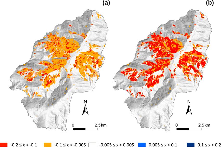
154                                                      S. Bernardie et al.: Modelling landslide hazards under global changes

Figure 2. Maps of existing and future land cover for the four scenarios in 2040 and 2100 (Houet et al., 2017).

of the roots is therefore taken into account as an additional            Table 3. Additional cohesion from each type of forest.
cohesion value. As roots can vary according to their orien-
tation, most studies consider their influence on the friction                Classification                 Principal type   Additional
angle of the material to be negligible (Norris et al., 2008).                (Houet et al., 2017)           of forest in      cohesion
Different models can be found for estimating cohesion; their                                                the area             (kPa)
quality varies and requires several types of biological input                No forest                      No forest                0
data (root resistance, root density and root morphology). Site
effects are also significant, making it impossible to find a sin-            Coniferous forest              Coniferous               8
gle value for cohesion for each species in the literature. When              Deciduous forest               Deciduous               12
the site conditions are not limiting, tree root systems are clas-
                                                                             Recolonization of the forest   Open                     5
sically categorized into three types: taproots, heart roots and
                                                                             (open and sparse)
flat roots. Wu et al. (1979) investigated how the three root
morphologies lead to breaks during a landslide and found
that pivoting systems are likely to mobilize the full potential
of root resistance because the stresses are concentrated on the             The depth of the influence of vegetation is limited by the
main root. On the other hand, for fasciculate and plate sys-             maximum extension of the roots; Bischetti et al. (2009) quote
tems, the stresses are distributed over the set of roots that are        Schiechtl (1980), who estimates that in mountainous terrain,
thinner and yield one after the other, which does not mobilize           the roots do not exceed 1 m in depth. This value is compa-
the full resistance potential of resistance of the system.               rable with those indicated by Crow (2005), who found that
   In the context of Cauterets, the presence or absence of a             90 % to 99 % of the root mass is less than 1 m deep. In this
forest constitutes the main parameter that may modify the                study, we considered the influence of vegetation to be limited
slope stability. This study considers four land cover types              to 1 m below the DTM.
that may have a significant influence on slope stability:                   Figure 3 shows the changes in the area of the four cate-
(a) no trees (urban areas, shrublands, natural grasslands, agri-         gories of land cover (coniferous, deciduous, open forest and
cultural areas and mineral surfaces), (b) coniferous forest,             no forest) for 2040 and 2100 in the fourth scenario; in 2010,
(c) deciduous forest and (d) encroachment (open forest).                 a majority of the area was composed of forest (52.0 %), with
   Table 3 summarizes the additional cohesion provided by                a balance between coniferous (19.3 %) and deciduous forests
each type of forest considered in the study area. The cohe-              (21.7 %) and a smaller open-forest area (11.0 %). The future
sion value for each type of forest is determined from Wu et              changes show a slight increase in the forested area in 2040
al. (1979) and Norris et al. (2008).                                     and a larger increase in 2100, regardless of the scenario. Con-
   The land cover in the current and future land cover maps              sidering the proportions of the different types of forest, the
were categorized according to these classifications.                     most important changes concern the scenarios of the aban-
                                                                         donment of the territory and sheep and woods. There is a de-

Nat. Hazards Earth Syst. Sci., 21, 147–169, 2021                                           https://doi.org/10.5194/nhess-21-147-2021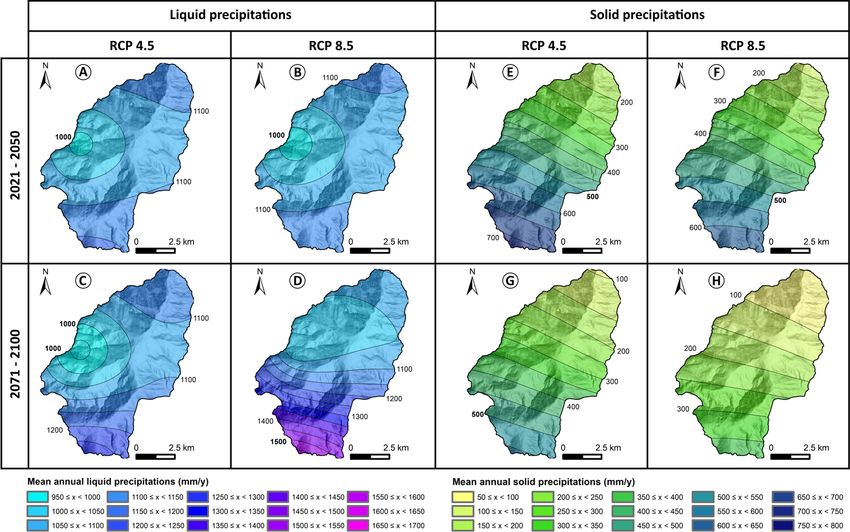
S. Bernardie et al.: Modelling landslide hazards under global changes 155
and (iii) long-term period, 2071–2100. A 30-year duration
is commonly used for meteorological parameters (e.g. pre-
cipitation) and defined according to WMO criteria (World
Meteorological Organization, 2018).
From a general point of view, the climate models show a
tendency toward an increase of the intensity of extreme pre-
cipitation events and annual cumulative precipitation in the
short and long term. The model results depend on the eleva-
tion of the area of interest. In the highest areas, the models
show an increase in cumulative precipitation. At the lowest
points, they indicate a slight increase in the short term and
a small decrease in the long term. Concerning the tempera-
ture, the models clearly indicate a significant increase in the
temperatures in the short (+1.54 ◦ C) and long term (+4 ◦ C),
resulting in large changes in the precipitation pattern (the
balance between snow and rainfall). Figure 4 shows that
both scenarios indicate the same tendency in the short term,
but they show some significant differences in the long term.
Moreover, there is a strong increase in liquid precipitation in
the long-term RCP8.5 scenario, coupled with a decrease in
solid precipitation over the same period. For the long-term
RCP4.5 scenario, liquid precipitation increases slightly com-
pared to that in the short term. The solid precipitation also
decreases for the same period.
With the GARDÉNIA model, which transforms precipi-
tation rates into water table variations, the daily water table
level is computed from the daily meteorological parameters.
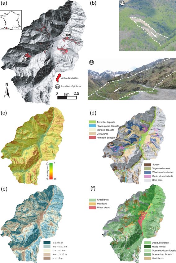
In this way, it is possible to obtain the distribution of the wa-
ter table level between low and high piezometric levels that
reflect the minimum and maximum indicators of the soil wa-
Figure 3. Evolution of land cover in 2010, 2040 and 2100 for the ter content (i.e. filling ratio). The piezometric level series,
four scenarios.
when converted into the water filling ratio, allows calcula-
tions to determine the water level class (WLC) and the as-
crease in open forest in the scenario of the abandonment of sociated frequency of occurrence, f (WLC), for each WLC.
the territory, whereas open forest increases for the scenario of Figure 5 shows the frequency distribution of the WLC of wa-
sheep and woods; in the scenario of the green town, the pro- ter level filling ratios for the current period (1981–2010), two
portions of the different land cover in 2040 remain similar future periods (2021–2050 and 2071–2100) and two climatic
to those in 2010, and the coniferous-forest surface increases scenarios (RCP4.5 and RCP8.5). This figure demonstrates
in 2100. Finally, the scenario of a renowned tourism resort the significant increase in the mean water table level in fu-
shows an increase in the area of coniferous and deciduous ture periods, especially between 2071 and 2100 under the
forests. most extreme scenario (RCP8.5).
4.2 Climate change scenarios and hydrogeological
inferences
5 Results
To take climate change into account, we selected two green-
house gas emissions scenarios, labelled in DRIAS (2014) 5.1 Landslide hazards in 2010
as RCP4.5 and RCP8.5 and computed using the ALADIN-
Climate model (ALADIN international team, 1997; Aire The objective of Fig. 6 is to demonstrate the sensitivity of the
Limitée Adaptation Dynamique Développement Interna- model to the evolution of the water filling ratio; thus for each
tional; International development for limited-area dynamical landslide type, 10 simulations were performed according to
adaptation) of Météo-France. the 10 ground water filling ratios (from 0 to 1). Figure 6 de-
Three periods were defined that are considered to be rep- picts the surface occupied by the different classes of hazards
resentative of the current year, 2050 and 2100: (i) refer- (according to FoS thresholds conventionally used for stabil-
ence period, 1981–2010; (ii) short-term period, 2021–2050; ity analyses; Kirsten, 1983; Pack et al., 2001; Table 4)
https://doi.org/10.5194/nhess-21-147-2021 Nat. Hazards Earth Syst. Sci., 21, 147–169, 2021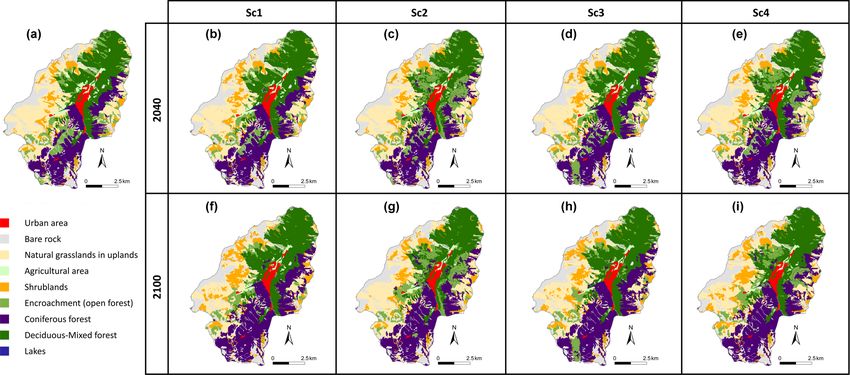
156                                                     S. Bernardie et al.: Modelling landslide hazards under global changes

Figure 4. Mean annual liquid and solid precipitation in the short and long term for RCP4.5 and RCP8.5 scenarios (from DRIAS, 2014).
For liquid precipitation: (a) 2021–2050 period, RCP4.5 scenario; (b) 2021–2050 period, RCP8.5 scenario; (c) 2071–2100 period, RCP4.5
scenario; and (d) 2071–2100 period, RCP8.5 scenario. For solid precipitation: (e) 2021–2050 period, RCP4.5 scenario ; (f) 2021–2050
period, RCP8.5 scenario; (g) 2071–2100 period, RCP4.5 scenario; and (h) 2071–2100 period, RCP8.5 scenario.

Figure 5. Frequency of the water table filling ratio.

Nat. Hazards Earth Syst. Sci., 21, 147–169, 2021                                     https://doi.org/10.5194/nhess-21-147-2021
S. Bernardie et al.: Modelling landslide hazards under global changes                                                              157

Table 4. Classes of hazards retained for the different computed       when the water table is high. This situation corresponds to
landslide hazard maps.                                                the different field observations. For shallow rotational land-
                                                                      slides, the simulated map does not recognize current unsta-
        Landslide hazard    Value of simulation expressed             ble surfaces very well; the relative error is high, ξ = 0.79.
        class                                      in FoS             However, the ROC (AUC) and PR (AUC) indexes show high
        Very high                               FoS ≤ 0.9             values. This is partly due to the low surface area of this
        High                              0.9 < FoS ≤ 1.1             type of landslide. For moderately deep rotational landslides,
        Moderate                         1.1 < FoS ≤ 1.35             the zones of depletion are well simulated by the model (i.e.
        Low                              1.35 < FoS ≤ 1.5             ξ = 0.37 and TPr = 66 %). Finally, for deep rotational land-
        Null                                    FoS > 1.5             slides, the relative error is relatively low (i.e. ξ = 0.35), and
                                                                      the ROC (AUC) and the prediction rate are high (i.e. ROC
                                                                      (AUC) = 0.82; PR (AUC) = 0.75). This means that the mod-
                                                                      els with such a water table level are able to simulate this par-
   As seen in Fig. 6, this analysis shows that the highly sus-        ticular type of landslide, which has a deep shear surface, well
ceptible surface areas are the largest for deep landslides and        and that the models are discriminating.
the smallest for shallow landslides.
   The relationship of the evolution of the hazard to the water
table level depends on the type of landslide.                         5.2     Future evolution of landslide hazards
   For the translational type (Fig. 6a), the graph indicates that
the area of the high hazard class is insignificant until a 0.6        5.2.1    Impacts of future land cover on landslide hazards
water filling ratio is reached; the hazard is then highly am-
plified with a strong increase in the areas of very high and
high landslide hazards. Similarly, for shallow rotational land-       Figure 9 shows maps of the differences in FoS values be-
slides (Fig. 6b), the area susceptible to landslides is very low      tween the current and future periods for the four socioeco-
at lower water filling ratios until the 0.5 value. At a water fill-   nomic scenarios and the two future periods, with the ob-
ing ratio of 0.8, there is a change in the evolution of the very      jective of specifically analysing the influence of future land
high and high hazard classes.                                         cover on landslide hazards. Climate conditions are consid-
   In contrast, the behaviour of moderately deep (Fig. 6c) and        ered equal between current and the two future periods and set
deep (Fig. 6d) landslides indicates a larger area of high haz-        to the actual conditions. This analysis was performed on shal-
ards: indeed, the area that is susceptible to landslides remains      low rotational landslides; this landslide type might be sensi-
higher than that for the shallow rotational landslides. The           tive to the evolution of land cover. In contrast, the stability of
area prone to landslides increases linearly with the lower wa-        deeper landslides is influenced by the effects of vegetation.
ter filling ratio values. The area then increases substantially          These maps indicate some differences between the current
at higher water filling ratios.                                       and future landslide hazards. These differences are character-
   In summary, a threshold of behaviour appears in the re-            ized by local increases and decreases in slope stability. These
sults, changing from low hazard levels and linear evolution           confined contrasts are significant, although they remain lim-
to higher hazard levels and exponential evolution with the            ited, as the change in the FoS ranges from −0.1 to +0.1,
water filling ratio; this threshold depends on the type of the        which is quite small.
landslide.                                                               When considering the impacts of future land cover on haz-
   Figure 7 illustrates landslide hazard maps for a conserva-         ard level changes in detail, we observe the following.
tive scenario based on a GWL of 0.9 to explain the land-                 In the scenario of the abandonment of the territory, we ob-
slide events observed in 1992 over the ski resort (Fig. 1B2)          serve a general increase in slope stability, which is in good
and over the Grange de Pan (Fig. 1B1). This type of situa-            accordance with the reduction in open forest highlighted in
tion, which corresponds to slope destabilization, is currently        Fig. 4. In the same way, the scenario of a renowned tourism
observed in moraine deposits overlapping weathering mate-             resort is characterized by an increase in stability, linked with
rials either in the French Pyrenees (Lebourg et al., 2003b)           the increase in deciduous and coniferous forests and very
or in the southern French Alps with similar geomorphologi-            limited areas of decreasing slope stability. In contrast, the
cal conditions (Thiery et al., 2017; Vandromme et al., 2020).         scenario of sheep and woods results in the destabilization
Each map shows the initiation areas of the different invento-         of some areas because of the development of open forest.
ried active landslides.                                               This scenario shows contrasting spatial evolution, as other
   The performance of the model is demonstrated through               areas become more stable. Finally, the scenario of the green
several statistical tests provided in Fig. 8. For shallow transla-    town results in more localized destabilization areas than the
tional landslides, the relative error is low (i.e. ξ = 0.21), and     scenario of sheep and woods, with patches of open forests
the true predictive rate is high (i.e. TPr = 0.80), indicating        and some improvement in stability in areas where coniferous
that the zones of depletion are well recognized by the model          forests are predicted to increase.

https://doi.org/10.5194/nhess-21-147-2021                                        Nat. Hazards Earth Syst. Sci., 21, 147–169, 2021
158 S. Bernardie et al.: Modelling landslide hazards under global changes
Figure 6. Evolution of the hazard level according to the water table level for the four types of landslides (2010): (a) translational, (b) shallow
rotational, (c) moderately deep rotational and (d) deep rotational.
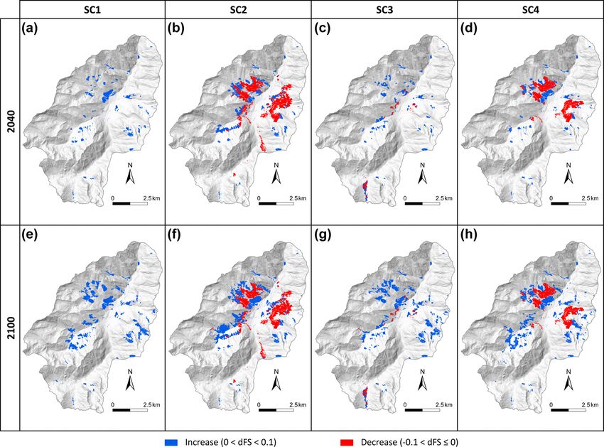
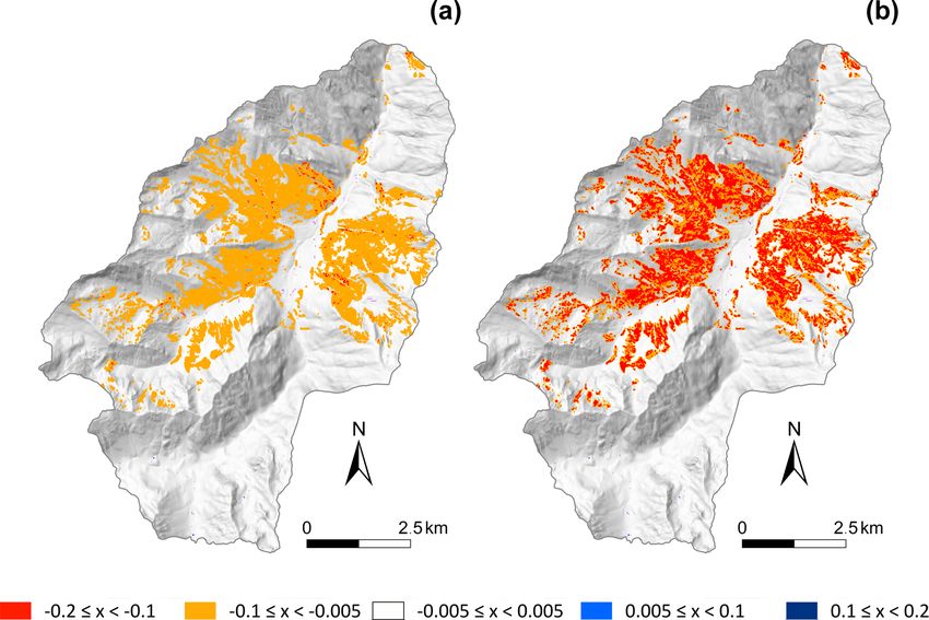
5.2.2 Impacts of future land cover and climate on Figures 10 and 11 show maps of the difference in the FoS
landslide hazards between the future (long term) and current periods for the
“shallow rotational” and “deep rotational” landscape types
We integrated climate change into the analysis of future land- under the two climate scenarios, RCP4.5 and RCP8.5. Even
slide hazards. Various analyses can be performed on the re- if all combinations of socioeconomic and climate scenarios
sults. In this paper, one of the indicators that we intend to have been computed, only one socioeconomic scenario is
quantify is the tendency of future hazard evolution. To this presented in this paper. Indeed, the results show that the ef-
end, we computed a “mean” of future landslide hazards. We fect of climate on landslide hazards is more significant than
computed the FoSMEAN indicator, which is the mean FoS the land cover. In these figures, the socioeconomic scenario
value for each cell in the studied area: of the abandonment of the territory is considered.
Xn Regardless of the scenario considered, there is a decrease
FoSMEAN = f (WLC) · FoS (WLC) ,
WLC=1 in slope stability. The FoS change ranges between −0.1 and
where WLC is the water level class; f (WLC) is the fre- −0.2. Therefore, even in a case where the future evolution of
quency of having the filling ratio equal to the WLC, as de- the forest stabilizes the slopes, the evolution of the ground-
termined in Fig. 5; and n is the number of filling ratio level water table destabilizes the area more.
classes, which is, in this case, is equal to 11 (see Fig. 5). In These figures can be more precisely analysed, as seen in
other words, we summed the hazard maps corresponding to Fig. 12, which provides the surface percentage for each haz-
the water table ratio, weighted according to the distribution ard class in the whole study area for each type of landslide,
of the water level filling ratio classes for the analysed period each climatic scenario and the two future periods. For clarity,
shown in Fig. 5. The final result of the process is a single the area corresponding to the very low hazard class has been
map that represents the mean landslide hazard over a given removed from the figures.
period.
Nat. Hazards Earth Syst. Sci., 21, 147–169, 2021 https://doi.org/10.5194/nhess-21-147-2021S. Bernardie et al.: Modelling landslide hazards under global changes 159
Figure 7. Landslide hazard map for 2010: (a) shallow translational, (b) shallow rotational, (c) moderately deep rotational, (d) deep rotational
and (e) all landslide types.
For the shallow rotational landslides, there is a strong in- 5.94 % in 2010 to 8.81 in 2040 (RCP8.5) and 8.84 % in 2100
crease of the medium hazard class, from 0.29 % to 3.23 % in (RCP8.5).
2040 for the RCP4.5 scenario; the high and very high classes
remain at the same very low level. Thus, the sum of the
surface classified in the three highest levels increases from 6 Discussion
0.34 % in 2010 to 2.12 % in 2040 (RCP8.5) and 2.78 % in
2100 (RCP8.5). This study analyses the evolution of future landslide hazards
For the translational landslides, the most important in- under the effects of land cover and climate changes. An ac-
crease occurs in the high hazard class, whereas there is a curate map provides a reference for establishing a compari-
decrease in the low hazard class, indicating that there is a son with the current state of landslide hazards. The criteria
transfer from low to medium and high classes. The total area computed to quantify the accuracy of the model permit the
classified in the three highest levels increases from 5.95 % validation of the model. For the four landslide types, the dif-
in 2010 to 8.04 % in 2040 (RCP8.5) and 8.49 % in 2100 ferent models computed for 2010 are considered represen-
(RCP8.5). The very high class remains at a very low level. tative of this Pyrenean mountainous context. The triggering
For the moderately deep landslides, some significant conditions used in the model are similar to those observed
changes are evident, with a large area of the low hazard class in the field and proposed by Fabre et al. (2002) and Lebourg
changing to the medium hazard class. The total area classi- et al. (2003a). The statistical results are satisfactory for each
fied in the three highest levels increases from 4.83 % in 2010 landslide type (e.g. the relative error ξ = 0.21 for the shallow
to 9.48 % in 2040 (RCP8.5) and 10.27 % in 2100 (RCP8.5). translational, ξ = 0.79 for the shallow rotational, ξ = 0.37
The deep landslides evolve differently, as the medium, for the moderately deep rotational and ξ = 0.35 for the deep
high and very high hazard levels increase significantly, from rotational). Even if the ξ for shallow rotational landslides is
slightly lower, we consider the results valid, as the majority
https://doi.org/10.5194/nhess-21-147-2021 Nat. Hazards Earth Syst. Sci., 21, 147–169, 2021160 S. Bernardie et al.: Modelling landslide hazards under global changes Figure 8. Statistic indicators between initiation areas and the very high and high hazard classes for (a) shallow translational, (b) shallow rotational, (c) moderately deep rotational and (d) deep rotational. of these landslides occur near torrents due to basal incision In contrast, apart from the impacts of land cover change on from the torrents. Hence, ALICE is not dedicated to simulat- landslide hazards, the quantification of future changes caused ing this specific mechanism, and the results do not indicate a by climate change indicates more significant changes in the high level of landslide hazards in these particular areas. size of the area that is susceptible to landslides; the size of All the results show that future global change scenarios this area depends on the landslide type considered. Com- imply significant evolution in landslide hazards, regardless of pared to the current period, the size of the area that is prone the climate scenario or the period considered. Generally, the to deep landslides is larger in the future than the area prone strongest effects on landslide hazards are linked to the evolu- to shallow landslides (both rotational and translational). On tion of the climate rather than the evolution of land cover; in- the other hand, the increase rate of areas prone to landslides deed, we have previously seen that, despite the incorporation is higher for the shallow landslide type than for the deep of the effects of land cover in the models, its impact remains landslide type; indeed, the area classified in the three highest quite limited, with an evolution of the FoS ranging from −0.1 hazard levels is projected to increase approximately 6-fold to +0.1. These limited changes are, however, significant, de- from 2010 to 2040 (RCP8.5) and 8-fold from 2010 to 2100 pending on the future land cover linked to the socioeconomic (RCP8.5) for shallow rotational landslides, whereas the area scenarios. In particular, the reduction in human presence (e.g. classified in the 3 highest hazard levels is projected to in- scenario of the abandonment of the territory) results in an in- crease approximately 1.5-fold from 2010 to 2040 (RCP8.5) crease in slope stability. In contrast, the increase in anthropic as well as to 2100 (RCP8.5) for deep rotational landslides. activity implies some contrasting evolutions of the area, with This result confirms the analyses of McInnes et al. (2007), some reduction in slope stability. The scenario of sheep and Moore et al. (2007), and Crozier (2010), which suggested woods illustrates this aspect, with the destabilization of ar- that the future evolution of landslide hazards in any environ- eas due to the development of open forest. These scenarios, ment depends on the type of landslide and in particular on its which represent four possible land cover evolution trajecto- depth and volume. ries, indicate contrasting spatial evolution patterns. Nat. Hazards Earth Syst. Sci., 21, 147–169, 2021 https://doi.org/10.5194/nhess-21-147-2021
S. Bernardie et al.: Modelling landslide hazards under global changes 161
Figure 9. Map of differences in FoS between current and future periods for the four scenarios and the two future periods: (a) abandonment
of the area in 2040, (b) sheep and woods in 2040, (c) a renowned tourism resort in 2040, (d) the green town in 2040, (e) abandonment of the
area in 2100, (f) sheep and woods in 2100, (g) a renowned tourism resort in 2100 and (h) the green town in 2100. The water table is constant.
Figure 12 reflects the mean tendency of the future scenar- corresponding to the 2071–2100 period (scenario RCP8.5)
ios within a 30-year period. Another feature to be analysed is (Figs. 13c, 14c and 15c) will increase 4-fold.
the occurrence frequency of landslide events. Indeed, as the These significant results have to be analysed in consider-
hydrogeological model considers the antecedent water con- ation of the tested hypotheses. Indeed, we have previously
tent, an increase in total rainfall implies that there will be seen that the effects of land cover on landslide hazards re-
an increase in the frequency of the highest water table level, mains quite limited. This may be inconsistent with some
as indicated in Fig. 5. As a result, when the antecedent wa- authors which explain that anthropic activities have a high
ter content is high, less water is required to trigger move- impact on the stability of slopes (Glade, 2003; Remondo
ment (Crozier, 2010). Therefore, landslides will occur more et al., 2005). Moreover, Crozier (2010) states “Changes re-
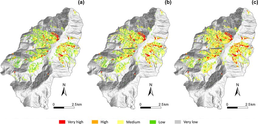
frequently. Figures 13, 14 and 15 correspond to the highest sulting from human activity are seen as a factor of equal,
frequency of the water filling ratio for each period (0.5 for if not greater, importance than climate change in affecting
the 1980–2010 period; 0.6 for the 2021–2050 period, sce- the temporal and spatial occurrence of landslides”. Several
nario RCP 8.5; and 0.7 for the 2071–2100 period, scenario features could explain such differences. Indeed, some land
RCP8.5). These results indicate that the highest frequency cover effects are considered in this study but not all. The ef-
of landslide hazards corresponding to the 2021–2050 period fects of the roots on slope stability is considered in the anal-
(scenario RCP8.5) (Figs. 13b, 14b and 15b) will increase ysis, but it could be more accurate to consider the effects of
1.5-fold, whereas the highest frequency of landslide hazards vegetation (suction and evapotranspiration) linked with the
runoff–infiltration balance, which is not spatially realized in
https://doi.org/10.5194/nhess-21-147-2021 Nat. Hazards Earth Syst. Sci., 21, 147–169, 2021You can also read