Sensitivity of the Antarctic ice sheets to the warming of marine isotope substage 11c
←
→
Page content transcription
If your browser does not render page correctly, please read the page content below
The Cryosphere, 15, 459–478, 2021
https://doi.org/10.5194/tc-15-459-2021
© Author(s) 2021. This work is distributed under
the Creative Commons Attribution 4.0 License.

Sensitivity of the Antarctic ice sheets to the
warming of marine isotope substage 11c
Martim Mas e Braga1,2 , Jorge Bernales3 , Matthias Prange3 , Arjen P. Stroeven1,2 , and Irina Rogozhina4
1 Geomorphology   and Glaciology, Department of Physical Geography, Stockholm University, Stockholm, Sweden
2 BolinCentre for Climate Research, Stockholm University, Stockholm, Sweden
3 MARUM – Center for Marine Environmental Sciences, University of Bremen, Bremen, Germany
4 Department of Geography, Norwegian University of Science and Technology, Trondheim, Norway

Correspondence: Martim Mas e Braga (martim.braga@natgeo.su.se)

Received: 20 April 2020 – Discussion started: 25 May 2020
Revised: 17 December 2020 – Accepted: 18 December 2020 – Published: 28 January 2021

Abstract. Studying the response of the Antarctic ice sheets          at intermediate depths, which leads to a collapse of the West
during periods when climate conditions were similar to the           Antarctic Ice Sheet if sustained for at least 4000 years.
present can provide important insights into current observed
changes and help identify natural drivers of ice sheet retreat.
In this context, the marine isotope substage 11c (MIS11c) in-
terglacial offers a suitable scenario, given that during its later   1   Introduction
portion orbital parameters were close to our current inter-
glacial. Ice core data indicate that warmer-than-present tem-        Lasting for as much as 30 kyr (thousand years), between
peratures lasted for longer than during other interglacials.         425 and 395 ka (thousand years ago), marine isotope sub-
However, the response of the Antarctic ice sheets and their          stage 11c (hereafter MIS11c) was the longest interglacial of
contribution to sea level rise remain unclear. We explore the        the Quaternary (Lisiecki and Raymo, 2005; Tzedakis et al.,
dynamics of the Antarctic ice sheets during this period using        2012). It also marked the transition from weaker to more
a numerical ice sheet model forced by MIS11c climate con-            pronounced glacial–interglacial cycles (EPICA Community
ditions derived from climate model outputs scaled by three           Members, 2004). Its long duration is attributed to a modu-
glaciological and one sedimentary proxy records of ice vol-          lation of the precession cycle, resulting in CO2 levels that
ume. Our results indicate that the East and West Antarctic ice       were high enough to suppress the cooling of the climate sys-
sheets contributed 4.0–8.2 m to the MIS11c sea level rise. In        tem due to the low eccentricity and thus reduced insolation
the case of a West Antarctic Ice Sheet collapse, which is the        (Hodell et al., 2000). Moreover, ocean sediment cores (e.g.
most probable scenario according to far-field sea level recon-       Hodell et al., 2000) and climate models (e.g. Rachmayani
structions, the range is reduced to 6.7–8.2 m independently          et al., 2017) show that the MIS11c global overturning cir-
of the choices of external sea level forcing and millennial-         culation was at an enhanced state, resulting in asynchronous
scale climate variability. Within this latter range, the main        warming of the southern and northern high latitudes (i.e. they
source of uncertainty arises from the sensitivity of the East        did not reach their warming peak at the same time; Steig and
Antarctic Ice Sheet to a choice of initial ice sheet configura-      Alley, 2002). However, Dutton et al. (2015) point out that cli-
tion. We found that the warmer regional climate signal cap-          mate modelling experiments with realistic orbital and green-
tured by Antarctic ice cores during peak MIS11c is crucial to        house gas forcings fail to fully capture this MIS11c warming
reproduce the contribution expected from Antarctica during           despite the fact that orbital parameters were almost identical
the recorded global sea level highstand. This climate signal         to present day (PD) during its late stage (EPICA Commu-
translates to a modest threshold of 0.4 ◦ C oceanic warming          nity Members, 2004; Raynaud et al., 2005). Earlier studies
                                                                     (e.g. Milker et al., 2013; Kleinen et al., 2014) have shown
                                                                     that climate models also tend to underestimate climate vari-

Published by Copernicus Publications on behalf of the European Geosciences Union.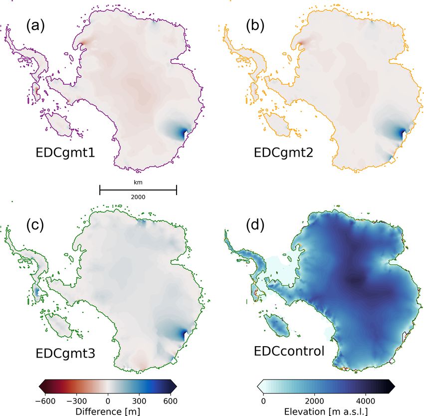
460          M. Mas e Braga et al.: Sensitivity of the Antarctic ice sheets to the warming of marine isotope substage 11c

ations during MIS11c, for which ice core reconstructions
show the mean annual atmospheric temperature over Antarc-
tica to have been about 2 ◦ C warmer than pre-industrial (PI)
values.
   A better understanding of the climate dynamics during
Quaternary interglacials, especially those that were warmer
than today, is critical because they can help assess Earth’s
natural response to future environmental conditions (Capron
et al., 2019). Among these periods, MIS5e (also referred to
as the Eemian, last interglacial, or LIG; Shackleton et al.,
2003) was originally proposed to be a possible analogue for
the future of our current interglacial (Kukla, 1997). More re-
cently, MIS11c has been considered another suitable candi-
date, since its orbital conditions were closest to PD (Berger
and Loutre, 2003; Loutre and Berger, 2003; Raynaud et al.,
2005). Furthermore, ice core evidence indicates that Termi-
nation V (i.e. the deglaciation that preceded MIS11) was
quite similar to the last deglaciation in terms of rates of         Figure 1. Surface topography of the AIS at the start of our core
change in temperature and greenhouse gas concentrations             experiments (425 ka), based on a calibration against Bedmap2,
                                                                    (Fretwell et al., 2013, see Sect. 2.1). Locations mentioned in the
(EPICA Community Members, 2004). The unusual length
                                                                    text are showcased, including the drilling sites of the ice cores used
of MIS11c and a transition to stronger glacial–interglacial         in this study (circles).
cycles seen in the subsequent geological record may have
been triggered by a reduced stability of the West Antarctic
Ice Sheet (WAIS, Fig. 1). The latter may have been due to the
cumulative effects of the ice sheet lowering its bed (Holden
et al., 2011), which in turn provided a positive climate feed-      tion, fuelling local glacier growth. Previous numerical mod-
back (Holden et al., 2010). The long duration of MIS11c was         elling experiments that encompass MIS11c also lack a con-
also shown to be a key condition to triggering the massive re-      sensus regarding AIS volume changes. For example, Sut-
treat of the Greenland Ice Sheet (GIS; Robinson et al., 2017).      ter et al. (2019) report an increased ice volume variability
Elucidating the response of the Antarctic ice sheet (AIS) to        from MIS11 (i.e. the isotopic stage in which MIS11c lies)
past interglacials can also help identify various triggers of ice   onwards, caused by stronger atmospheric and oceanic tem-
sheet retreat. This is because each interglacial has its unique     perature variations, while Tigchelaar et al. (2018) only ob-
characteristics: for example, while MIS11c was longer than          tained significant volume changes during the last 800 kyr
the LIG, the latter was significantly warmer (Lisiecki and          when increasing their ocean temperatures to values as high
Raymo, 2005; Dutton et al., 2015).                                  as 4 ◦ C. Conversely, de Boer et al. (2013) report higher sea
   The MIS11c history of Antarctica is less constrained than        level contributions during MIS15e, MIS13, and MIS9 and
that of Greenland (e.g. Willerslev et al., 2007; Reyes et al.,      weaker contributions during MIS11c and MIS5e. Among the
2014; Dutton et al., 2015; Robinson et al., 2017). Whereas          past interglacials, the LIG and the Pliocene are considered
Raymo and Mitrovica (2012) consider that the WAIS had col-          to be the closest analogues to MIS11c, and studies acknowl-
lapsed and that the East Antarctic Ice Sheet (EAIS, Fig. 1)         edge the possibility of a WAIS collapse in both periods (e.g.
provided a minor contribution based on their estimate of            Hearty et al., 2007; Naish et al., 2009; Pollard and DeConto,
MIS11c global sea levels of 6 to 13 m above PD, studies di-         2009). However, Pliocene model results were shown to be
rectly assessing the AIS response have been elusive. For ex-        highly dependent on the choice of climate and ice sheet mod-
ample, sedimentary evidence has been inconclusive regard-           els (de Boer et al., 2015; Dolan et al., 2018).
ing the possibility of a collapse of the WAIS during some              Constraints are also scarce for the MIS11c climate, and its
Quaternary interglacials (Hillenbrand et al., 2002, 2009;           heterogeneity is reflected in the ice core records. Reconstruc-
Scherer, 2003), and evidence for the instability of marine          tions from different ice cores located in East Antarctica (cir-
sectors of the EAIS has only recently been provided (Wilson         cles in Fig. 1) show different histories regarding the evolution
et al., 2018; Blackburn et al., 2020). Counter-intuitively, the     of atmospheric surface temperature. For example, the Vostok
dating of onshore moraines in the Dry Valleys to MIS11c,            ice core surface air temperature reconstruction (Petit et al.,
indicating local ice advance, has been used to indirectly           1999; Bazin et al., 2013) reveals a weak temperature peak
support regional ice sheet retreat (Swanger et al., 2017).          (about 1.6 ◦ C above PI around 410 ka) compared to those of
Swanger et al. (2017) argue that ice sheet retreat in the           EPICA Dome C (EDC; over 2.7 ◦ C above PI around 406 ka,
Ross Embayment provided nearby open-water conditions                Jouzel et al., 2007) and Dome Fuji (DF; 2.5 ◦ C above PI
and therefore a source of moisture and enhanced precipita-          around 407 ka, Uemura et al., 2018). The latter two ice core

The Cryosphere, 15, 459–478, 2021                                                          https://doi.org/10.5194/tc-15-459-2021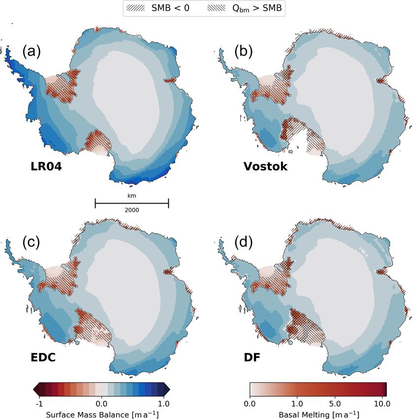
M. Mas e Braga et al.: Sensitivity of the Antarctic ice sheets to the warming of marine isotope substage 11c                   461

records also present a peak-warming period of much longer          correctly track the position of the cold–temperate transition
duration (ca. 15 kyr compared to 7 kyr at Vostok).                 in the thermal structure of a polythermal ice body.
   As detailed, many modelling studies have investigated AIS          The model combines the shallow-ice approximation (SIA)
responses over time periods that include MIS11. However, so        and shelfy-stream approximation (SStA) using (see Bernales
far none has focused specifically on this period. Given the        et al., 2017b, Eq. 1)
scarce information for MIS11c and conflicting constraints
on how Antarctica responded to this exceptionally long in-         U = (1 − w) · usia + ussta ,                                (1)
terglacial (Milker et al., 2013; Dutton et al., 2015), we here
focus on the peak-warming period between 420 and 394 ka.           where U is the resulting hybrid velocity, usia and ussta are the
Our aim is to reduce the current uncertainties in the AIS be-      SIA and SStA horizontal velocities, respectively, and w is a
haviour during MIS11c, addressing the following questions.         weight computed as
                                                                                                     !
    1. How did the AIS respond to the warming of MIS11c?                         2         |ussta |2
                                                                   w (|ussta |) = arctan               ,                        (2)
       More specifically, what are the uncertainties in the AIS                  π           u2ref
       minimum configuration, timing, and potential sea level
       contribution?                                               where the reference velocity uref is set to 30 m a−1 , mark-
                                                                   ing the transition between slow and fast ice. This hybrid
    2. What was the main driver of the changes in the AIS          scheme reduces the contribution from SIA velocities mostly
       volume? Was it warming duration, peak temperature,          in coastal areas of fast ice flow and heterogeneous topogra-
       changes in precipitation, or changes in the oceanic forc-   phy, where this approximation becomes invalid. Basal slid-
       ing?                                                        ing is implemented within the computation of SStA veloc-
   Ice sheet model simulations depend on applied forcings,         ities as a Weertman-type law (see Bernales et al., 2017a,
boundary conditions, and parameterisations for a wide range        Eqs. 2–6). The amount of sliding is controlled by a tem-
of processes. Such parameters control, for example, basal          porally fixed, spatially varying map of friction coefficients
sliding, ice deformation, bedrock deformation, ice shelf basal     that was iteratively adjusted during an initial present-day
melting, and ice shelf calving. The sensitivity of ice volume      equilibrium run (Pollard and DeConto, 2012b), such that
changes across glacial–interglacial timescales to model pa-        the grounded ice thickness matches the present-day obser-
rameters was extensively explored by Albrecht et al. (2020).       vations from Bedmap2 (Fretwell et al., 2013) as close as
DeConto and Pollard (2016) carried out a large ensemble            possible. Sliding coefficients in sub-ice-shelf and ocean ar-
analysis for the LIG and the Pliocene, where parameters re-        eas are set to 105 m a−1 Pa−1 , representing soft, deformable
lated to ice shelf loss were constrained according to their        sediment, in the event the grounded ice advances over this
ability to simulate target ranges of sea level contribution.       region. The initial bedrock, ice base, and ocean floor eleva-
Simpler flow-line models have also been used to evaluate un-       tions are also taken from Bedmap2. Enhancement factors for
certainties in basal conditions (Gladstone et al., 2017) and       both grounded and floating ice are set to 1, based on sensi-
flow law parameters (Zeitz et al., 2020). Here, we perform         tivity tests in Bernales et al. (2017b). This choice provides
five ensembles of experiments that focus on choices that           the best match between observed and modelled ice thickness
are external to the numerical model and could help guide           for this hybrid scheme, similar to the findings in Pollard and
other modelling efforts on the choice of forcings and bound-       DeConto (2012a).
ary conditions. We evaluate the impact of the following on            Surface mass balance is calculated as the difference be-
AIS volume and extent during MIS11c: the choice of proxy           tween accumulation and surface melting. The latter is com-
record (including their differences in signal intensity and        puted using a semi-analytical solution of the positive degree
structure), the choice of sea level reconstruction, and uncer-     day (PDD) model following Calov and Greve (2005). Near-
tainties in assumptions regarding the geometry of the AIS at       surface air temperatures entering the PDD scheme are ad-
the start of MIS11c.                                               justed through a lapse rate correction of 8.0 ◦ C km−1 to ac-
                                                                   count for differences between the modelled ice sheet topog-
                                                                   raphy and that used in the climate model from which the air
2     Methods                                                      temperatures are taken. For the basal mass balance of ice
                                                                   shelves, we use a calibration scheme of basal melting rates
2.1    Ice sheet model                                             developed in Bernales et al. (2017b) to optimise a parameter-
                                                                   isation based on Beckmann and Goosse (2003) and Martin
For our experiments we employ the 3D thermomechanical              et al. (2011) that assumes a quadratic dependence on ocean
polythermal ice sheet model SICOPOLIS (Greve, 1997; Sato           thermal forcing (Holland et al., 2008; Pollard and DeConto,
and Greve, 2012) with a 20 km horizontal grid resolution and       2012a; Favier et al., 2019). This optimised parameterisation
81 terrain-following vertical layers. It uses the one-layer en-    is able to respond to variations in the applied glacial index
thalpy scheme of Greve and Blatter (2016), which is able to        (GI, Sect. 2.2) forcing. A more detailed description of this

https://doi.org/10.5194/tc-15-459-2021                                                      The Cryosphere, 15, 459–478, 2021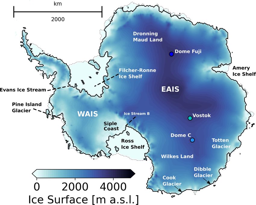
462          M. Mas e Braga et al.: Sensitivity of the Antarctic ice sheets to the warming of marine isotope substage 11c

Table 1. Main parameters used in the experiments.

                           Parameter    Name                                            Value    Units
                           Egrounded    Enhancement factor (grounded ice)                   1    –
                           Efloating    Enhancement factor (ice shelves)                    1    –
                           n            Glen’s flow law exponent                            3    –
                           p            Weertman’s law p exponent                           3    –
                           q            Weertman’s law q exponent                           2    –
                           τ            ELRA model time lag                                 1    kyr
                           D            ELRA model flexural rigidity               2.0 × 1025    Nm
                           γlr          Lapse rate correction                             8.0    ◦ C km−1

                           S0           Sea water salinity                                 35    –
                           ρsw          Sea water density                                1028    kg m−3
                           ρice         Ice density                                       910    kg m−3
                           cp0          Ocean mixed layer specific heat capacity         3974    J kg−1 K−1
                           γT           Thermal change velocity                         10−4     m s−1
                           Li           Latent heat of fusion                      3.35 × 10⁵    J kg−1 K−1

parameterisation is given in Sect. S1 of the Supplement. In            tialise the AIS by performing a thermal spin-up over a period
our experiments, we prescribe a time lag of 300 years for              of 195 kyr from 620 to 425 ka; i.e. we apply a transient sur-
the ocean response to GI variations, which is considered the           face temperature signal from the EDC ice core (Jouzel et al.,
most likely lag in response time of the ocean compared to the          2007) as an anomaly to our PI climate (described in the next
atmosphere in the Southern Ocean (Yang and Zhu, 2011).                 section) while keeping the ice sheet geometry constant at our
At the grounding line, the basal mass balance of partially             previously calibrated Bedmap2-based configuration. We then
floating grid cells is computed as the average melting of the          let the AIS freely evolve for 5 kyr, between 425 and 420 ka,
surrounding, fully floating cells, multiplied by a factor be-          applying transient GI forcing during the relaxation period
tween 0 and 1 that depends on the fraction of the cell that            (Fig. S12). We chose 425 ka as the starting point for relax-
is floating. This fraction is computed using an estimate of            ation because it is when the MIS11c oxygen isotope values
the sub-grid grounding line position based on an interpo-              in the EDC ice core are closest to PI. When analysing the re-
lation of the current, modelled bedrock and ice shelf basal            sults, we ignore the first 5 kyr (425–420 ka) to avoid a shock
topographies. At the ice shelf fronts, calving events are pa-          from suddenly letting the ice sheet topography freely evolve
rameterised through a simple thickness threshold, where ice            at the start of our period of interest. Figure 1 shows the ther-
thinner than 50 m is instantly calved away.                            mally spun-up ice sheet configuration at 425 ka, from which
   Bed deformation is implemented using a simple elastic               the simulations start. The EDC ice core was chosen for the
lithosphere, relaxing asthenosphere (ELRA) model, with a               thermal spin-up and as common forcing for all ensemble runs
time lag of 1 kyr and flexural rigidity of 2.0 × 1025 N m,             except for CFEN, where we test different core-derived cli-
which Konrad et al. (2014) found to best reproduce the re-             mate signals (see below), because it spans the longest period
sults of a fully coupled ice-sheet–self-gravitating viscoelas-         among the three ice cores tested while still providing a rela-
tic solid Earth model. The geothermal heat flux applied at the         tively high temporal resolution.
base of the lithosphere is taken from Maule et al. (2005) and
is kept constant. All relevant parameters used in the mod-             2.2   Climate forcing and core experiments
elling experiments are listed in Table 1.
   Sea level contribution at a given time step is computed in          In an effort to assess the impact of similarities and differences
SICOPOLIS as the difference in total ice volume above flota-           in existing paleoclimate reconstructions, and regional differ-
tion between the ice sheet at the time step and the spun-up            ences in the ice core records, we perform an ensemble of sim-
pre-industrial ice sheet. When computing ice volume, differ-           ulations where each member is forced by a GI (Eq. 3) derived
ences in bedrock elevation between the two ice sheets are              from δD from ice cores or δ 18 O from the LR04 stack of deep-
accounted for by using a common reference bedrock eleva-               sea sediment cores (Fig. 2a; Petit et al., 2001; EPICA Com-
tion in all time steps. We also correct for the projection effect      munity Members, 2004; Lisiecki and Raymo, 2005; Uemura
on the horizontal grid area.                                           et al., 2018). Since an ensemble of fully coupled climate-
   All ensembles cover a period from 420 to 394 ka. After              ice sheet model runs over 26 kyr is at present computation-
the calibration for basal sliding mentioned above, we ini-             ally challenging, an evaluation of possible scenarios for the
                                                                       peak-temperature response during MIS11c based on the pa-

The Cryosphere, 15, 459–478, 2021                                                           https://doi.org/10.5194/tc-15-459-2021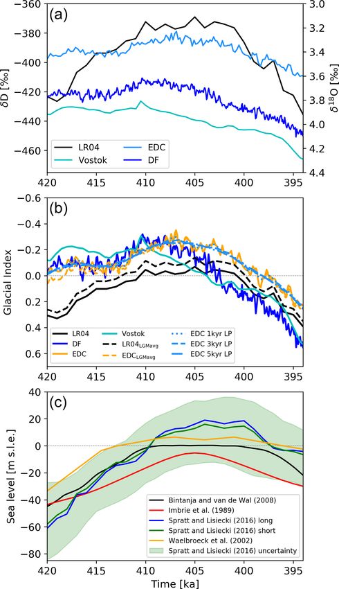
M. Mas e Braga et al.: Sensitivity of the Antarctic ice sheets to the warming of marine isotope substage 11c                            463

Table 2. Ice and sediment cores reference values used in Eq. (3), together with the age (in thousand years before present; ka) from which the
Last Glacial Maximum (LGM) reference values were obtained. The respective age models of each core, and their references, are listed.

              Record     Type (isotope)         δXPI     δXLGM      Age     Age model     Reference
                                                 [‰]        [‰]     (ka)
              EDC        Ice (δD)            −397.4      −449.3     24.0    EDC3          EPICA Community Members (2004)
              DF         Ice (δD)            −425.3      −469.5     22.8    AICC2012      Uemura et al. (2018)
              Vostok     Ice (δD)            −440.9      −488.3     24.4    GT4           Petit et al. (2001)
              LR04       Sediment (δ 18 O)     3.23        4.99     20.0    LR04          Lisiecki and Raymo (2005)

                                                                           leoclimate signals from different ice sheet sectors can be a
                                                                           cheaper yet effective approach. The GI method is a way of
                                                                           weighting the contributions from interglacial (PI) and full
                                                                           glacial (Last Glacial Maximum; LGM) average states. It does
                                                                           so by rescaling a variable curve (usually temperature or iso-
                                                                           tope reconstructions from an ice or sediment record) based
                                                                           on reference PI and LGM values, which consider PI climate
                                                                           as GI = 0 and LGM climate as GI = 1 (Eq. 3):

                                                                                      δX(t) − δXPI
                                                                           GI(t) =                 ,                                     (3)
                                                                                     δXLGM − δXPI
                                                                           where t is time, and X is deuterium for the ice cores or
                                                                           18 O  for sediment cores. The value for δXPI was obtained
                                                                           as the average of the last 1000 years before 1850 CE, while
                                                                           δXLGM was taken as the minimum and maximum value
                                                                           for δD and δ 18 O, respectively, between 19 and 26.5 ka (Clark
                                                                           et al., 2009; Clason et al., 2014). For our two reference cli-
                                                                           mate states (i.e. PI and LGM), we use the Community Cli-
                                                                           mate System Model version 3 (CCSM3) PI time slice in
                                                                           Rachmayani et al. (2016) and the LGM time slice in Han-
                                                                           diani et al. (2013), which used identical model versions and
                                                                           were run on the same platform. A brief assessment of the
                                                                           model biases against PD data is provided (Sects. S2 and S3).
                                                                           The atmospheric and ocean temperature (T ) fields at time t
                                                                           are reconstructed based on their respective PI and LGM ref-
                                                                           erence fields (TPI and TLGM respectively) using (see also
                                                                           Fig. S13)

                                                                           T (t) = TPI + GI(t) · (TLGM − TPI ) ,                         (4)

                                                                           while precipitation is given by an exponential function to pre-
                                                                           vent negative values and to ensure a smooth transition be-
                                                                           tween the PI and LGM states
                                                                                     1−GI(t)      GI(t)
                                                                           P (t) = PPI         · PLGM .                                  (5)

                                                                           The PI and LGM reference values (including the reference
Figure 2. Reconstructions used in this study: (a) LR04 δ 18 O (black)      ages for the latter) for the three ice cores and the LR04 stack
and Vostok, Dome C (EDC), and Dome Fuji (DF) ice core δD [‰];              are summarised in Table 2, together with their respective
(b) resulting glacial indices from the reconstructions in panel (a)        age models. The ensemble of simulations forced by different
(see Sect. 2 and Table 3 for the legends); (c) global mean sea level       GI curves (Climate Forcing ENsemble, CFEN) constitutes
anomaly relative to PI (metre sea level equivalent, m s.l.e.).             our core experiments.

https://doi.org/10.5194/tc-15-459-2021                                                                The Cryosphere, 15, 459–478, 2021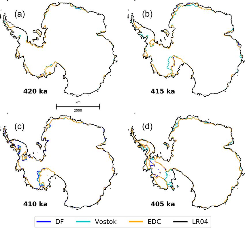
464           M. Mas e Braga et al.: Sensitivity of the Antarctic ice sheets to the warming of marine isotope substage 11c

2.3     Sensitivity experiments                                    different sea level reconstructions, the Sea Level Sensitivity
                                                                   ENsemble (SLSEN).
2.3.1    Sensitivity to the GI scaling
                                                                   2.3.4   Sensitivity to the choice of initial ice sheet
Because different approaches have been used to transform                   geometry
the isotope curves into a GI, we assess the sensitivity to the
choice of the scaling procedure by performing an additional        Similar studies that assess AIS changes over glacial and in-
scaling using another reference value for δXLGM . In the new       terglacial cycles often adopt a PI or PD starting geometry
scaling procedure, δXLGM is the average (between 19 and            (e.g. Sutter et al., 2019; Tigchelaar et al., 2019; Albrecht
26.5 ka) rather than the peak value. We compare the effects        et al., 2020). We have followed the same approach in our
of using these two procedures when applied to the EDC ice          CFEN experiments (see Sect. 2.2). Although the similarity
core δD and the LR04 stack δ 18 O records (orange and black        to the modern AIS configuration has been loosely inferred
dashed lines in Fig. 2b respectively). We call this ensemble       from sedimentary (Capron et al., 2019) and ice core (EPICA
the Scaling Sensitivity ENsemble (SSEN).                           Community Members, 2004) proxy records, to our knowl-
                                                                   edge there is no direct evidence to support this claim (e.g.
2.3.2    Sensitivity to millennial-scale variability               Swanger et al., 2017). Hence, we also perform an ensemble
                                                                   of simulations starting from different ice sheet geometries.
Given the different temporal resolutions of climate records,       This allows for an evaluation of the influence of an initial
lower-resolution reconstructions such as LR04 and Vostok           AIS configuration at 420 ka on its modelled retreat and ad-
might not capture the impact of millennial variability or          vance (including possible thresholds) and provides an uncer-
shorter events, as do EDC and DF (Fig. 2a). Thus, we as-           tainty envelope in its potential sea level contribution based
sess the potential effects of record data resolution and mil-      on this criterion. We call this the Starting Geometry Sensitiv-
lennial (or shorter) timescale variability by applying 1, 3, and   ity ENsemble (SGSEN), and its three unique geometries are
5 kyr low-pass filters to the EDC ice core GI and forcing our      forced with the ice core reconstructed climate forcings tested
model with the resulting smoothed GI curves (light blue lines      in CFEN.
in Fig. 2b). We then compare these three simulations to the           In order to create a representative range of initial geome-
original EDC-derived ice sheet history and call this ensemble      tries at 420 ka, we use a common starting geometry but vary
the Resolution Sensitivity ENsemble (RSEN).                        the relaxation time. For this purpose, we first create an an-
                                                                   cillary geometry by perturbing the thermally spun-up AIS
2.3.3    Sensitivity to sea level                                  with a constant LGM climate (air temperature and precipita-
                                                                   tion rates) and no sub-ice-shelf melting over a 5 kyr period.
Sea level plays an important role in determining the flotation     The resulting ancillary ice sheet (which has an extent that sits
of the ice sheet and the stresses at its marine margins. Un-       between PI and LGM configurations) is then placed at 420,
certainties in global mean sea level reconstructions are there-    425, and 430 ka and runs transiently (following the respec-
fore a significant concern, and several studies have indeed fo-    tive GIs) until 394 ka. This creates a representative range
cused on improving their estimates (e.g. Imbrie et al., 1989;      of starting geometries at 420 ka (Fig. 3), and each initial ice
Waelbroeck et al., 2002; Bintanja and van de Wal, 2008;            sheet geometry is labelled gmt1 to gmt3 (Fig. 3a–c; the short-
Spratt and Lisiecki, 2016, Fig. 2c). We evaluate the effect        est relaxation is gmt1 and the longest is gmt3). The gmt1 ini-
of using a particular sea level reconstruction on the evolution    tial topography is generally more extensive and thinner than
of the AIS by running an ensemble of simulations with EDC-         the control. Its grounding line advanced at the southern mar-
derived GI, where each member uses a different sea level re-       gin of the Filchner–Ronne Ice Shelf and at Siple Coast, but
construction. For each ensemble member, the sea level forc-        the ice sheet interior is on average 200 m thinner than the
ing applied at the boundaries of the ice sheet is approximated     control and up to 500 m thinner across particular regions such
to the global mean sea level of its respective sea level re-       as the dome areas of the WAIS and Wilkes Land (Dome C). It
construction. Sea level curves included in this ensemble are       is, however, about 200 m thicker at its fringes, which results
three of the reconstructions presented by Spratt and Lisiecki      in a gentler surface gradient towards the ice sheet margins.
(2016), termed “long” (i.e. uses records that extend as far        The gmt2 initial topography is less than 100 m thinner than
back as 798 ka), “short” (uses records that extend at least un-    the control over the EAIS interior and about 100 m thicker
til 430 ka), and the “upper uncertainty boundary” from their       over the WAIS interior and at the EAIS margins. Finally, the
records, because we consider their lower uncertainty bound-        gmt3 initial topography is overall thicker than the control,
ary to be satisfactorily covered by SPECMAP (Imbrie et al.,        though not by more than 100 m except at the western side of
1989), which we include. We also include in the analysis the       the Antarctic Peninsula and the WAIS margins, where some
reconstructions from Bintanja and van de Wal (2008) and            regions are up to 300 m thicker (Fig. 3c). Table 3 summarises
from Waelbroeck et al. (2002). All these records are pre-          all experiments described in this section.
sented in Fig. 2c, and we call this ensemble, where we test

The Cryosphere, 15, 459–478, 2021                                                       https://doi.org/10.5194/tc-15-459-2021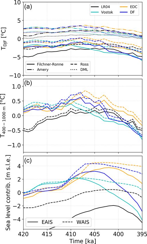
M. Mas e Braga et al.: Sensitivity of the Antarctic ice sheets to the warming of marine isotope substage 11c 465
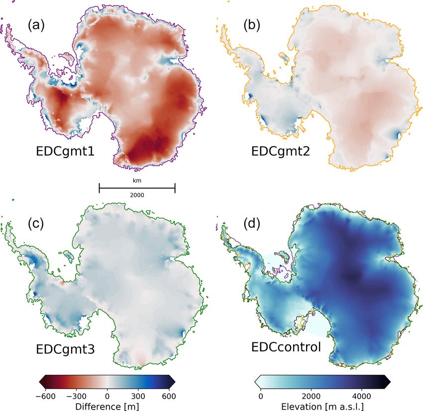
Figure 3. (a–c) Three different starting ice sheet geometries at 420 ka for gmt1–3 using EDC forcing. The EDC CFEN member is used
as control. The same spatial pattern is seen for DF and Vostok cases, and the averaged ice elevation difference between their respective
geometries amounts to less than 50 m. The colour scheme shows differences in surface elevation between each geometry and the control for
420 ka (d). Differences are only shown where the ice is grounded in both geometries, and coloured lines show the respective grounding lines
in gmt1–3, also overlain in panel (d).
3 Results about 412 ka. Subsequently, the peak warming starts and per-
sists (in a slightly warmer state than reconstructed with Vos-
3.1 Climate forcing reconstructions tok after 410 ka) until 397 ka. Its rate of decline after 404 ka
is similar to the Vostok and LR04 curves, although it is in
Considering the four adopted isotope curves (Fig. 2a and b), a warmer state. Finally, the DF reconstruction is somewhere
although similar at first sight, the GI reconstructions are dif- in between the other two ice cores (Fig. 2b). It shows quite
ferent from one another and therefore offer a range of mod- stable conditions at the start (i.e. no pronounced warming),
elled ice sheet responses. The LR04 GI reconstruction is rising to a rather pronounced warming peak similar in struc-
generally colder, showing conditions warmer than PI only ture to the EDC reconstruction, but peaks at 410 ka, similar
for the warmest period of MIS11c (i.e. between ca. 410 and to the Vostok curve. Finally, its rate of decline is similar to
400 ka). Consequently, it does not show a peak warming as the other cores and so it crosses PI values (GI = 0) later than
strong as the other reconstructions (Fig. 2b). Although the the Vostok but earlier than the EDC curves, between 404 and
ice cores have similar ranges in GI values and similar over- 403 ka.
all aspects of the curves (and good covariance between EDC The ice sheet history for MIS11c using the LR04 forcing
and DF; Uemura et al., 2018), they differ in key aspects. is clearly different from the others. The ice sheet loses less
The Vostok reconstruction starts at a warmer state than the than a third of its volume compared to the other CFEN mem-
others at 420 ka, has a modest peak warming at 410 ka, and bers and becomes smaller than PD for a duration of 9 kyr,
then consistently declines towards a colder state (crossing the while the others are consistently below PD levels (Fig. 4a).
GI = 0 line at about 404 ka). The EDC reconstruction shows It is worth reminding that, in contrast to other members of
a mildly-warmer-than-PI state at 420 ka, which persists until
https://doi.org/10.5194/tc-15-459-2021 The Cryosphere, 15, 459–478, 2021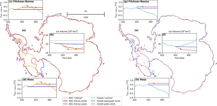
466          M. Mas e Braga et al.: Sensitivity of the Antarctic ice sheets to the warming of marine isotope substage 11c

Table 3. Summary of performed experiments grouped by ensemble, listing their respective GI forcings, applied sea level reconstruction,
and choice of initial geometry. LGMavg denotes that the GI was rescaled using the average LGM value as opposed to the peak value
(see Sect. 2.3.1 and Table 4). The SGSEN experiments were grouped for better visualisation, but each SGSEN row corresponds to three
experiments, one starting from each geometry (gmt1–3).

           Ensemble     Experiment      GI forcing                  Sea level reconstruction                       Initial
                                                                                                                   geometry
           CFEN         lr04            LR04                        Bintanja and van de Wal (2008)                 control
           CFEN         edc             EDC                         Bintanja and van de Wal (2008)                 control
           CFEN         df              DF                          Bintanja and van de Wal (2008)                 control
           CFEN         vos             Vostok                      Bintanja and van de Wal (2008)                 control
           SSEN         lr04lgmavg      LR04LGMavg                  Bintanja and van de Wal (2008)                 control
           SSEN         edclgmavg       EDCLGMavg                   Bintanja and van de Wal (2008)                 control
           RSEN         lp1bx           EDC (1 kyr low pass, LP)    Bintanja and van de Wal (2008)                 control
           RSEN         lp3bx           EDC (3 kyr low pass, LP)    Bintanja and van de Wal (2008)                 control
           RSEN         lp5bx           EDC (5 kyr low pass, LP)    Bintanja and van de Wal (2008)                 control
           SLSEN        s16l            EDC                         Spratt and Lisiecki (2016) long                control
           SLSEN        s16s            EDC                         Spratt and Lisiecki (2016) short               control
           SLSEN        s16u            EDC                         Spratt and Lisiecki (2016) upper uncertainty   control
           SLSEN        spm             EDC                         Imbrie et al. (1989)                           control
           SLSEN        wae             EDC                         Waelbroeck et al. (2002)                       control
           SGSEN        edcgmt[1–3]     EDC                         Bintanja and van de Wal (2008)                 gmt1–3
           SGSEN        dfgmt[1–3]      DF                          Bintanja and van de Wal (2008)                 gmt1–3
           SGSEN        vosgmt[1–3]     Vostok                      Bintanja and van de Wal (2008)                 gmt1–3

CFEN, the LR04 curve starts with colder-than-PI conditions            3.2   Sensitivity to rescaling of the climate forcings
and does not produce a peak warming as strong as the others.
It only shows a brief period of warmer-than-PI conditions be-         The different δ isotope reference values used for the SSEN
tween 410 and 401 ka (Fig. 2b), resulting in an overall larger        experiments are shown in Table 4 (cf. Table 2). Using an
AIS (Fig. 5). The ice core CFEN members yield lower ice               LGM-averaged value results in a smaller ice sheet for the
volumes throughout the entire MIS11c (Fig. 4a) but with im-           LR04 GI, while for the EDC GI it results in a slightly larger
portant variations. The Vostok-forced experiment, for exam-           AIS than their correspondent CFEN experiments through-
ple, suffers a faster ice loss at the beginning of the simulation     out the entire MIS11c (Fig. 4b). The LR04-LGM-averaged
period, when it shows a sudden warming. However, it recov-            run, however, still does not produce AIS retreat as signifi-
ers more quickly than the EDC and DF experiments as soon              cant as the other experiments, with 4.2 % less volume (1.1 ×
as the peak warming is over and the climate starts to shift           106 km3 ) at 402 ka when compared to its original rescaling.
back to PI conditions, without a WAIS collapse (we consider           The warmer conditions resulting from the GI rescaling are
the WAIS to have collapsed when the Weddell, Ross, and                still not enough to compensate for the initial growth caused
Amundsen seas become interconnected; Fig. 5).                         by significantly-colder-than-PI conditions at 420 ka and dur-
   The members that result in a collapse of the WAIS (forced          ing the preceding relaxation stage. Although differences in
with the DF and EDC reconstructions) reveal slightly differ-          ice sheet volumes exist between the different scaling strate-
ent responses (Fig. 4a). The experiment forced by the EDC             gies in the EDC-forced experiments, the resulting ice sheet
reconstruction shows an AIS volume reduction after a sud-             histories are quite similar. Despite ice sheet volume at 402 ka
den warming at around 418 ka, but the WAIS collapse is de-            being smaller in the run where the LGM reference is taken as
layed until 407–406 ka (Fig. 5), following a second short pe-         the peak value, the differently scaled ice sheet is only 1.2 %
riod with an increased warming rate after 412 ka, which leads         larger in volume than the CFEN ice sheet (0.3 × 10⁶ km3 ).
up to the peak warming of MIS11c. The DF experiment on
the other hand is rather stable until 412 ka, when the climate
starts warming towards its peak. Most of the retreat is trig-
gered after the sudden temperature rise at 412 ka, as opposed
to when the peak warming occurs.

The Cryosphere, 15, 459–478, 2021                                                              https://doi.org/10.5194/tc-15-459-2021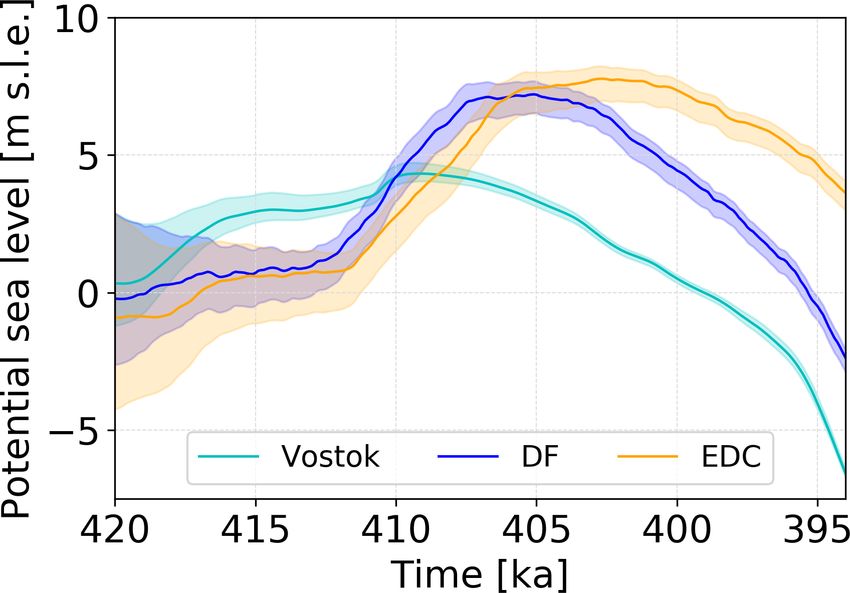
M. Mas e Braga et al.: Sensitivity of the Antarctic ice sheets to the warming of marine isotope substage 11c                          467

                                                                        Table 4. Different isotope values adopted for the GI rescaling pro-
                                                                        cedure. LGMavg is the reference value obtained from the average
                                                                        between 26 and 19.5 ka (which replaces LGM in Eq. 3 for the re-
                                                                        spective experiments; see Sect. 2.3.1).

                                                                                   Record       δXPI     δXLGM      δXLGMavg
                                                                                                 [‰]        [‰]         [‰]
                                                                                   EDC        −397.4     −449.3        −442.3
                                                                                   LR04         3.23       4.99          4.85

                                                                        volumes between ensemble members (the volume is larger
                                                                        the more filtered the forcing is), it is negligible compared
                                                                        to the overall changes in volume experienced by the entire
                                                                        ensemble.
                                                                           Although the range of global mean sea level reconstruc-
                                                                        tions is wide (nearly reaching 60 m between 405 and 400 ka;
                                                                        Fig. 2c), the AIS response in terms of volume is remarkably
                                                                        similar for different sea level curves (Fig. 4e). The differ-
                                                                        ences in sea level have their largest impacts on the volume
                                                                        of floating ice (Fig. 4d). Thus, floating ice volume directly
                                                                        reflects the sea level forcing effect on the flotation of ice
                                                                        and consequently on the grounding line position. The SLSEN
                                                                        member with the highest sea level rise (i.e. the upper uncer-
                                                                        tainty boundary of Spratt and Lisiecki, 2016) deviates the
                                                                        most from the other members, especially in the portion of
                                                                        grounded ice being brought to flotation (Fig. 4d). However,
                                                                        the differences are not significant enough to yield substan-
                                                                        tially distinct ice volume changes (Fig. 4e).

                                                                        3.4   Sensitivity to the choice of initial ice sheet geometry

                                                                        Looking at how the four initial geometries (gmt1–3 and the
                                                                        control) evolve under the three different climate forcings
                                                                        from the ice-core-derived GI reconstructions (Fig. 6), it be-
                                                                        comes clear that all members under the same climate forc-
                                                                        ing have a tendency to follow the same path despite differ-
                                                                        ing initial ice sheet configurations. The spread in minimum
                                                                        ice sheet volumes (and consequently implications for WAIS
Figure 4. Sensitivity of AIS response (in total ice volume, 106 km3 )   collapse) due to assumptions of starting geometry becomes
between 420 and 394 ka to (a) CFEN GI reconstructions, (b) SSEN         rather small, between 1 and 3 m s.l.e. at 405 ka among the
rescaled GI reconstructions, and (c) RSEN low-pass filtered GI re-      three different forcings in SGSEN. The different ice sheet
constructions. Panels (d) and (e) show floating and total ice volumes   configurations also show a similar pacing of retreat after
(in 106 km3 ), respectively, for the SLSEN sea level forcing recon-     412 ka, indicating that their corresponding volume by that
structions forced by EDC GI (see Table 3). The dashed line shows        time did not affect its rate of retreat due to climate warming.
PD ice volume (Fretwell et al., 2013).                                  In our SGSEN simulations, it appears that the main source
                                                                        of variability between ice sheets with different initial geome-
                                                                        tries comes from specific EAIS drainage basins, such as those
3.3   Sensitivity to millennial variability and sea level               of Cook, Totten, and Dibble glaciers (Fig. 7 showcases the
      reconstructions                                                   EDC ensemble; cf. Fig. 1 for geographical locations). The
                                                                        latter two remain thicker in the alternative geometry experi-
The trajectories of each ensemble member in RSEN agree                  ments than in the correspondent CFEN experiment, whereas
with one another (Fig. 4c), showing increased delays in the             the former is thinner in gmt3 (Fig. 7c). Some variability can
ice sheet retreat in response to the filtering intensity. Also,         also be observed in the WAIS domain. Parts of Pine Island
although it is possible to see slight differences in ice sheet          Glacier appear to resist ice sheet collapse in the thicker-ice-

https://doi.org/10.5194/tc-15-459-2021                                                           The Cryosphere, 15, 459–478, 2021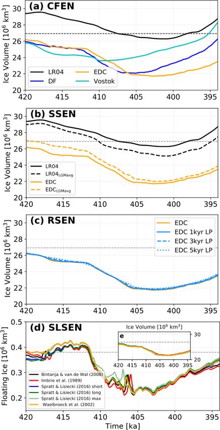
468          M. Mas e Braga et al.: Sensitivity of the Antarctic ice sheets to the warming of marine isotope substage 11c

Figure 5. Grounding lines at 420, 415, 410, and 405 ka for the CFEN simulations.

geometry experiments (gmt3) when compared to the CFEN-
equivalent run (Fig. 7c and d). Given the observed spread, the
three ensemble members constrain the range of potential sea
level contributions from Antarctica during the MIS11c high-
stand to 4.0–8.2 m (minimum from Vostok at 410 ka, max-
imum from EDC at 405 ka). This range of 4.2 m essentially
corresponds to whether the WAIS has collapsed or not during
MIS11c.

4   Discussion

Our simulations show that during the peak of MIS11c the
WAIS probably collapsed. We base this statement on results
from experiments forced by different proxy records with
significant differences in their structure during the MIS11c          Figure 6. Sensitivity of the AIS response to CFEN GI recon-
peak warming. One consisted of a short single peak (Vos-              structions (Vostok, DF, EDC) between 420 and 394 ka with uncer-
                                                                      tainty bands from four distinct initial ice sheet starting geometries
tok), while others showed a prolonged period of (relatively)
                                                                      (gmt1–3 and respective CFEN member), expressed in contribution
warmer conditions (LR04, DF, and EDC). Despite having                 to global mean sea level [m s.l.e.]. Solid lines show the mean of each
a warming peak of a similar GI magnitude at 410 ka, the               common-forcing ensemble member, while the colour filling shows
Vostok-forced CFEN member is the only ice-core-forced en-             the spread given by the different starting geometries.
semble member that shows no collapse of the WAIS. Al-
though the remaining climate reconstructions all show a
longer peak, differences still exist among them. For exam-
ple, EDC and DF, which are the most similar to each other,

The Cryosphere, 15, 459–478, 2021                                                            https://doi.org/10.5194/tc-15-459-2021
M. Mas e Braga et al.: Sensitivity of the Antarctic ice sheets to the warming of marine isotope substage 11c 469 Figure 7. (a–c) Ice sheet geometries at 405 ka for the EDC CFEN member using three different starting geometries at 420 ka (Fig. 3). The colour scheme shows differences in surface elevation between each geometry and the control for 405 ka (d). Differences are only shown where the ice is grounded in both geometries, and coloured lines show the respective grounding lines in gmt1–3, also overlain in panel (d). start shifting to their warmest conditions at about the same Finally, LR04 stands out when compared to the ice cores and time around 414 ka but peak at different times. DF peaks at will be discussed in more detail separately. 410 ka, which is 3 kyr earlier than EDC. Regardless of this Although sensitivity experiments show WAIS-collapse re- difference, the simulated WAIS collapse occurs at 407 ka sults using DF and EDC to be robust, the timing of the events using the DF and at 406 ka using the EDC core forcing, discussed above should be taken with caution for two main which is closer than their timing of peak warming. Ex- reasons. First, we are forcing the entire AIS model with a periments forced by both records also yielded similar ice climate signal from the EAIS while previous studies have volumes (Fig. 4a) and extents (Fig. 5). It should be men- shown that the WAIS could have responded over 2 kyr ear- tioned that the combination of GI and climate model forc- lier to changes in climate (WAIS Divide Project Members, ing results in a warmer signal in the surface temperatures 2013). Second, all discrepancies in the timing of the events at the DF, EDC, and Vostok core sites than obtained di- discussed so far recorded by the ice core records, especially rectly from their δD records (Fig. S14). This is most likely the peak warming and ice sheet collapse, are within the un- due to the LGM cold bias in CCSM3, which persisted de- certainty in their respective age models (Parrenin et al., 2007; spite the lapse rate correction applied. Since PI tempera- Bazin et al., 2013). Consequently, these two factors prevent tures do not have any strong bias, the LGM cold bias causes us from establishing an exact timing of these events, which the GI reconstruction to yield colder temperatures during means that the lags in AIS response are the most important colder-than-PI times (GI > 0) and warmer temperatures dur- to be considered. ing warmer-than-PI times (GI < 0). Nevertheless, Vostok’s In all our CFEN simulations, ice sheet retreat is associ- GI-reconstructed temperature peak matches the peak ob- ated with stronger basal melting close to grounding lines, es- served in DF for its δD-derived curve and is also close to the pecially at Siple Coast, and the Ross and Filchner–Ronne warmest temperature reconstructed with the EDC isotopes. ice shelves (Fig. 8). Surface ablation seems to be signifi- https://doi.org/10.5194/tc-15-459-2021 The Cryosphere, 15, 459–478, 2021
470          M. Mas e Braga et al.: Sensitivity of the Antarctic ice sheets to the warming of marine isotope substage 11c

Figure 8. Surface mass balance (SMB, m a−1 ) for the grounded ice and basal melting (Qbm , m a−1 ) for the ice shelves for the CFEN
simulations at 415 ka. Hatched areas show where basal melting dominates over surface mass balance and where surface mass balance is
negative (i.e. where surface ablation occurs).

cant only over the fringes of the EAIS, notably at Dron-            Amery Ice Shelf), ice shelves are small and provide little
ning Maud Land (DML) and the Amery Ice Shelf, where                 buttressing. Hence, because most of the EAIS is grounded
surface temperatures reach positive values during summer            above sea level, its sub-shelf melting is not high enough to
(Fig. 9a). Nevertheless, they show limited retreat compared         force grounding line retreat as strongly as in the WAIS. As
to the aforementioned WAIS ice shelves. The strong WAIS             a consequence, ice melt is dominated by surface ablation at
retreat seen in the EDC- and DF-forced runs starting from           the ice sheet fringes (compare hatched patterns in Fig. 8).
412 ka is triggered by an increase in ocean temperatures at in-        The average intermediate-depth ocean temperatures un-
termediate depths (hereafter defined as the average between         der the Filchner–Ronne and Ross ice shelves peak between
400 and 1000 m depth) under the Ross and Filchner–Ronne             0.4 and 0.85 ◦ C for the three ice-core-forced CFEN mem-
ice shelves (Fig. 9b). Although this increase is progressive,       bers (Fig. 9b). This happens at 410 ka for Vostok, 408 ka
it triggers a faster loss of volume by the WAIS compared to         for DF, and 407 ka for EDC. Strong WAIS retreat, however,
the EAIS after 412 ka (Fig. 9c), in contrast with a similar         starts before the peak in forcing, supporting the presence of
evolution between the ice sheets before then. This observed         a tipping point at 412 ka. To further test whether this tipping
tipping point at 412 ka also explains why the different ini-        point is the trigger of WAIS collapse, we have performed four
tial ice sheet configurations under a common forcing follow         additional experiments: (i) forced by EDC GI, but keeping
the same trend from that moment onwards (Fig. 6) and why            the GI constant after 416 ka (i.e. before the threshold found
the evolution of WAIS and EAIS sea level contributions di-          in ocean temperatures); (ii) forced by EDC GI, but keep-
verges. As ocean forcing becomes the main driver of ice sheet       ing the GI constant after 410 ka (i.e. just after the sudden
retreat, it has a much larger impact on marine-based portions       increase in ocean temperatures but before the maximum is
of the ice sheet. Around most of the EAIS (except for the           reached; Fig. 9b); (iii) forced by Vostok GI, where climate

The Cryosphere, 15, 459–478, 2021                                                       https://doi.org/10.5194/tc-15-459-2021
M. Mas e Braga et al.: Sensitivity of the Antarctic ice sheets to the warming of marine isotope substage 11c                       471

                                                                       this threshold must be sustained for at least 4 kyr to cause
                                                                       a collapse (cf. red and blue dashed lines in Fig. 10f–h). A
                                                                       short peak at this threshold and subsequent cooling prevents
                                                                       the WAIS from collapsing, compared to keeping it constant at
                                                                       the same peak value (Fig. 10e and f). Comparing these values
                                                                       to PI temperatures averaged over the same extent of the wa-
                                                                       ter column, the magnitude of warming necessary to cross this
                                                                       threshold is 0.4 ◦ C. In other words, a warming of this magni-
                                                                       tude can be understood as the condition necessary for WAIS
                                                                       collapse (Fig. 10c, d, g and h). Additional experiments where
                                                                       we test for a weakened ocean forcing further confirm this
                                                                       threshold, as a complete collapse of the WAIS is prevented
                                                                       when the temperatures at intermediate depths fail to reach a
                                                                       0.4 ◦ C warming relative to PI under the Filchner–Ronne and
                                                                       Ross ice shelves (Sect. S4). Considering that the tempera-
                                                                       ture peak reconstructed by the Vostok GI is the closest to the
                                                                       δD-derived temperature peaks in DF and EDC (Fig. S14), a
                                                                       more prolonged warming as seen in the DF and EDC ice core
                                                                       seems to be a crucial condition for the modelled WAIS draw-
                                                                       down during MIS11c. For example, if the GI-derived tem-
                                                                       perature for DF was not overestimated and had its peak value
                                                                       close to its isotope-derived value, the response would likely
                                                                       resemble the experiment where Vostok-peak conditions were
                                                                       kept constant from 410 ka onwards.
                                                                          The inferred critical warming of intermediate-depth ocean
                                                                       temperatures of 0.4 ◦ C for MIS11c is close to the equilib-
                                                                       rium model results in Garbe et al. (2020) but lower than re-
                                                                       sults from Turney et al. (2020) for the AIS retreat during the
                                                                       LIG. While the former study shows a strong WAIS retreat
                                                                       is already possible for an ocean warming of 0.7 ◦ C, the lat-
                                                                       ter identifies a tipping point at 2 ◦ C warming in ocean tem-
                                                                       peratures. In other interglacials, such as the LIG, the shorter
                                                                       duration but higher intensity of ocean warming compared to
                                                                       MIS11c could have triggered WAIS collapse (Dutton et al.,
Figure 9. Evolution throughout MIS11c for each CFEN member
                                                                       2015; Turney et al., 2020), since a stronger rate of warm-
for (a) summer surface air temperature [◦ C] averaged over the main
Antarctic ice shelves, (b) ocean temperatures averaged between
                                                                       ing can drive ice retreat at a much faster pace. Thus, WAIS
400 and 1000 m [◦ C] for the Filchner–Ronne and Ross ice shelves,      collapse during MIS11c was likely attained because ocean
and (c) sea level contribution by EAIS and WAIS. Colours denote        temperatures exceeded a modest threshold for long enough
the respective CFEN member, while line styles in panels (a) and (b)    (over 4 kyr).
denote each ice shelf and each ice sheet in panel (c). DML refers to      Despite differences in the model sensitivity to ocean tem-
all smaller ice shelves along the Dronning Maud Land margin.           perature, our results support those of Tigchelaar et al. (2019)
                                                                       and Albrecht et al. (2020) regarding the minor role that vari-
                                                                       ations in sea level play in driving ice sheet retreat compared
forcing is kept constant at its peak condition at 410 ka; and          to other external forcings. Although the coarse treatment of
(iv) forced by Vostok GI, where, after the 410 ka peak, GI is          the grounding lines could have had an influence on the seem-
brought back to its 411 ka value (i.e. between the peak and            ing insensitivity of our experiments to sea level uncertainties,
the observed tipping point) and kept constant. Figure 10a              other models of similar resolution which apply different sub-
and b show that keeping the EDC-derived climate constant               grid parameterisations to the grounding lines yield similar
at 416 ka conditions prevents the WAIS from collapsing,                results (Tigchelaar et al., 2019; Sutter et al., 2019; Albrecht
while keeping it constant at 410 ka conditions delays its col-         et al., 2020). Hence, while this caveat must be taken into con-
lapse by almost 5 kyr compared to the core CFEN run. The               sideration, it does not appear to have influenced our results
Vostok-based simulations (Fig. 10e–h) show that there is in-           dramatically.
deed a threshold in ocean temperatures, which is approxi-                 Moreover, AIS minimum extent and the timing of WAIS
mately 0.45 ◦ C for the Filchner–Ronne ice shelf and 0.54 ◦ C          collapse are robust regardless of model resolution (Fig. S15).
for the Ross ice shelf. However, our results also imply that           A set of simulations performed with several resolutions

https://doi.org/10.5194/tc-15-459-2021                                                         The Cryosphere, 15, 459–478, 2021
472 M. Mas e Braga et al.: Sensitivity of the Antarctic ice sheets to the warming of marine isotope substage 11c Figure 10. Thresholds for WAIS collapse. (a, e) Grounding lines at 405 ka for three EDC-based (solid lines) and three Vostok-based (dashed lines) experiments, respectively (see below for explanation); (b, f) ice volume (106 km3 ), (c, d, g, h) intermediate-depth (400–1000 m) ocean temperatures [◦ C] for the Filchner–Ronne and Ross ice shelves, respectively. Time series cover the period between 420 and 395 ka for both EDC-based (solid lines) and Vostok-based (dashed lines) experiments. The orange line shows the EDC control run, while the cyan line shows the Vostok control run. Blue lines show EDC and Vostok simulations where climate was kept constant and the WAIS did not collapse, while the red lines show EDC and Vostok simulations where climate was kept constant and the WAIS collapsed. Yellow circles show the moment when the WAIS breaks down and an open-water connection between the Ross, Weddell, and Amundsen seas is established. (from 20 to 10 km) showed virtually the same changes in ilar to the Holocene during MIS11c (Lisiecki and Raymo, ice sheet extent and modest variations in ice volume, which 2005) despite the geological evidence that there was a contri- amount to a spread of 1.2 m s.l.e. in sea level contribution at bution to higher-than-Holocene sea levels from both Green- 405 ka. Alternative sliding laws or sub-shelf melting param- land and Antarctica (Scherer et al., 1998; Raymo and Mitro- eterisations, for example using a linear dependence of sub- vica, 2012). Hence, the inclusion of many Northern Hemi- shelf melt to ocean thermal forcing, or applying a more phys- sphere records in the LR04 stack explains why it fails to ically realistic approach (e.g. Reese et al., 2018) were not capture the Antarctic warming during MIS11c seen in the tested and could influence our results. For example, numer- ice cores and the differences in timing compared to them. ical modelling studies in which the WAIS did not collapse This also helps explain why the different criteria adopted during MIS11c were acknowledged to be less sensitive to for changing its scaling procedure had little effect on the re- the ability of ocean temperatures to drive basal melting (Pol- sults (Fig. 4b). A possible way of circumventing this prob- lard and DeConto, 2009; Tigchelaar et al., 2019). Finally, we lem could be to adopt a similar scaling approach to Sutter note that, despite very different approaches in reconstructing et al. (2019), who combined the LR04 stack and EDC ice transient signals, neither Pollard and DeConto (2009) nor we core temperature records, which, in their study, also led to were able to simulate a collapse of the WAIS using the LR04 WAIS collapse during MIS11c. stack as climate forcing. In East Antarctica, our simulations do not capture the ice The LR04 reconstruction is composed of a stack of sheet retreat into the Wilkes Subglacial Basin recently pro- 57 globally distributed ocean sediment cores (Lisiecki and posed by Wilson et al. (2018) and Blackburn et al. (2020) Raymo, 2005), with a strong deficit over the Southern Ocean. for MIS11. Blackburn et al. (2020) suggest this retreat to In the Nordic Seas, paleoceanographic records indicate that have been caused by ocean warming, with little to no atmo- the ocean was colder than present during MIS11 (Bauch spheric influence. However, further paleoceanographic data et al., 2000; Kandiano et al., 2016; Doherty and Thibodeau, are needed to fully understand this retreat (Noble et al., 2018). Colder ocean temperatures in the Northern Hemi- 2020), which so far has not been captured by other model sphere explain why LR04 shows oxygen isotopic values sim- experiments (see Wilson et al., 2018, Fig. 2b). As for West The Cryosphere, 15, 459–478, 2021 https://doi.org/10.5194/tc-15-459-2021
M. Mas e Braga et al.: Sensitivity of the Antarctic ice sheets to the warming of marine isotope substage 11c                     473

Antarctica, far-field sea level reconstructions suggest that a
WAIS collapse was the most probable scenario (Raymo and
Mitrovica, 2012; Chen et al., 2014) when comparing global
highstand estimates with the probable contribution from the
GIS. While Robinson et al. (2017) found that Greenland
contributed between 3.9 and 7.0 m to sea level rise (hav-
ing 6.1 m s.l.e. as the most likely value), the AIS contribu-
tion cannot be constrained by simply subtracting the GIS’s
contribution from the global sea level highstand. The sug-
gested asynchronicity between the GIS and AIS minimum
extents (Steig and Alley, 2002) and the uncertainties in the
age models of the different analysed ice cores (Petit et al.,
1999; Parrenin et al., 2007; Bazin et al., 2013) prevent a sim-
ple relationship between both ice sheet records to be estab-        Figure 11. Sea level contribution (in m s.l.e.) of each SGSEN mem-
lished. Based on the ice core experiments, our range for the        ber during the global sea level highstand (405 ka for EDC and DF,
potential sea level contribution of the AIS is 4.0–8.2 m. This      410 ka for Vostok).
wide range is mainly related to whether the WAIS collapses
or not. Considering the cases where the WAIS collapsed (i.e.
EDC and DF ice core experiments) as the most probable sce-          knowledge no special focus has been given to Antarctica’s
nario, our range for the potential sea level contribution of        response to the peak warming during MIS11c and the driv-
the AIS is 6.7–8.2 m. In this case, the EAIS contribution is        ing mechanisms behind it. To fill this gap we evaluated the
the largest source of uncertainty, being most sensitive to the      deglaciation of Antarctica using a numerical ice sheet model
choice of starting ice geometry. This effect is strongest over      forced by a combination of climate model time slice forcing
Wilkes Land, where the spread in position of the grounding          and various transient records through a glacial index (GI).
line is wider, and ice thickness is more variable than for other    The records were obtained from ice cores of the EAIS inte-
basins (Fig. 7). While nearby drainage basins, such as those        rior and a stacked record of deep-sea sediment cores taken
of Totten and Dibble glaciers, become more stable given the         from far-field regions. We evaluated the sensitivity of our re-
larger ice sheet configurations of the alternative geometries       sults to (i) the scaling of the GI, (ii) millennial variability
(Fig. 3b and c), Cook Glacier, emanating from the Wilkes            and temporal record resolution, (iii) different sea level recon-
Subglacial Basin, appears to thin regardless of the choice of       structions, and (iv) initial ice sheet configurations. While sea
initial geometry (Fig. 7a–c). Overall, the EAIS contributes         level, higher-frequency variability, and the GI scaling of the
1.7 to 3.7 m s.l.e. during the highstand (Fig. 11). Conversely,     records seemed to play a small role, different responses were
the WAIS was rather insensitive to the choice of starting ge-       seen for both East and West Antarctic ice sheets regarding
ometry (yielding 4.3–4.5 m s.l.e. during the highstand in the       the different applied transient signals and for the initial ice
case of a collapse and 2.0–2.2 otherwise) due to the stronger       sheet configurations. Among the applied ice core reconstruc-
role played by the sub-shelf ocean forcing after 412 ka. There      tions, the warming captured by the Vostok ice core during
are, however, two stabilising feedbacks which are not incor-        MIS11c was not strong enough to cause a collapse of the
porated in our model: (i) a local sea level drop caused by a        WAIS, which was attributed to the short duration of its peak.
reduced gravitational attraction of a shrinking ice sheet (e.g.     Our results indicate that our modelled WAIS collapse was
Mitrovica et al., 2009) and (ii) the observed faster rebound of     caused by the duration rather than the intensity of warming
the crust due to a lower mantle viscosity in some WAIS loca-        and that it was insensitive to the choice of the starting geom-
tions (Barletta et al., 2018). The first effect is probably small   etry. The latter proved to be a larger source of uncertainty for
based on our model’s insensitivity to sea level changes over        the EAIS. Regarding the initial questions posed in the begin-
these timescales, but we have been unable to robustly test the      ning of this study, we now provide short answers to them:
effect of a faster rebound on AIS response during MIS11c.
However, we note that our ELRA model is set up with a rel-            1. How did the AIS respond to the warming of MIS11c?
atively short response time of 1 kyr, for which the resulting            What are the uncertainties in the AIS minimum configu-
bedrock uplift is still not able to trigger a stabilising effect         ration, its timing, and potential sea level contribution?
large enough to prevent WAIS collapse.
                                                                         Using transient signals from EAIS ice cores, we
                                                                         found a range in sea level contribution of 4.0 to
5   Conclusions                                                          8.2 m s.l.e., which mainly reflects whether the WAIS
                                                                         has collapsed or not in our experiments. For the former
Several studies have been carried out in order to reconstruct            scenario – which is supported by far-field sea level
past ice changes over the Antarctic continent, but to our                reconstructions – we find that a WAIS collapse during

https://doi.org/10.5194/tc-15-459-2021                                                       The Cryosphere, 15, 459–478, 2021
You can also read