Summer aerosol measurements over the East Antarctic seasonal ice zone
←
→
Page content transcription
If your browser does not render page correctly, please read the page content below
Atmos. Chem. Phys., 21, 9497–9513, 2021
https://doi.org/10.5194/acp-21-9497-2021
© Author(s) 2021. This work is distributed under
the Creative Commons Attribution 4.0 License.

Summer aerosol measurements over the East Antarctic
seasonal ice zone
Jack B. Simmons1 , Ruhi S. Humphries2,3 , Stephen R. Wilson1 , Scott D. Chambers4 , Alastair G. Williams4 ,
Alan D. Griffiths4,1 , Ian M. McRobert5 , Jason P. Ward2 , Melita D. Keywood2,3 , and Sean Gribben2
1 Centre for Atmospheric Chemistry, School of Earth, Atmospheric and Life Sciences, University of Wollongong,
Wollongong, NSW 2522, Australia
2 Climate Science Centre, CSIRO Oceans and Atmosphere, Aspendale, VIC 3195, Australia
3 Australian Antarctic Program Partnership, University of Tasmania, Hobart, TAS 7000, Australia
4 ANSTO, Environmental Research, Locked Bag 2001, Kirrawee DC, NSW 2232, Australia
5 Engineering and Technology Program, CSIRO National Research Collections Australia, Hobart, TAS 7004, Australia

Correspondence: Jack B. Simmons (js828@uowmail.edu.au)

Received: 25 November 2020 – Discussion started: 26 November 2020
Revised: 29 April 2021 – Accepted: 3 May 2021 – Published: 23 June 2021

Abstract. Aerosol measurements over the Southern Ocean          rections suggests the influence of large-scale atmospheric
have been identified as critical to an improved understanding   transport mechanisms on the local aerosol population in the
of aerosol–radiation and aerosol–cloud interactions, as there   boundary layer of the East Antarctic seasonal ice zone. Mod-
currently exists significant discrepancies between model re-    elled back trajectories imply different air mass histories for
sults and measurements in this region. The atmosphere above     each measurement group, supporting this suggestion. CN3
the Southern Ocean provides crucial insight into an aerosol     and CCN concentrations were higher during periods where
regime relatively free from anthropogenic influence, yet        the absolute humidity was less than 4.3 gH2 O /m3 , indica-
its remoteness ensures atmospheric measurements are rel-        tive of free tropospheric or Antarctic continental air masses,
atively rare. Here we present observations from the Polar       compared to other periods of the voyage. Increased aerosol
Cell Aerosol Nucleation (PCAN) campaign, hosted aboard          concentration in air masses originating close to the Antarc-
the RV Investigator during a summer (January–March) 2017        tic coastline have been observed in numerous other studies.
voyage from Hobart, Australia, to the East Antarctic sea-       However, the smaller changes observed in the present anal-
sonal sea ice zone. A median particle number concentra-         yses suggest seasonal differences in atmospheric circulation,
tion (condensation nuclei > 3 nm; CN3 ) of 354 (95 % CI         including lesser impact of synoptic low-pressure systems in
345–363) cm−3 was observed from the voyage. Median              summer. Further measurements in the region are required be-
cloud condensation nuclei (CCN) concentrations were 167         fore a more comprehensive picture of atmospheric circula-
(95 % CI 158–176) cm−3 . Measured particle size distribu-       tion in this region can be captured and its influence on local
tions suggested that aerosol populations had undergone sig-     aerosol populations understood.
nificant cloud processing. To understand the variability in
aerosol observations, measurements were classified by me-
teorological variables. Wind direction and absolute humid-
ity were used to identify different air masses, and aerosol     1   Introduction
measurements were compared based on these identifica-
tions. CN3 concentrations measured during SE wind direc-        Aerosol–radiation and aerosol–cloud interactions are among
tions (median 594 cm−3 ) were higher than those measured        the most uncertain parameters in the current estimates of
during wind directions from the NW (median 265 cm−3 ).          global radiative forcing (Carslaw et al., 2013; Myhre et al.,
Increased frequency of measurements from these wind di-         2013) and hence a major uncertainty in calculating the cli-
                                                                mate effects of changing atmospheric composition. In partic-

Published by Copernicus Publications on behalf of the European Geosciences Union.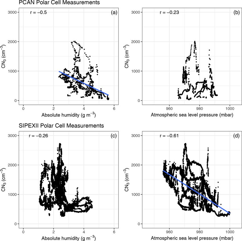
9498                                                                   J. B. Simmons et al.: Summer aerosol measurements

ular, there is a need for reliable estimates for aerosol load-     wood, 2017), Macquarie Island (54.5◦ S 158.9◦ E) (Brech-
ings in the pre-industrial atmosphere, as this is the reference    tel et al., 1998), and Dumont D’Urville Station, Antarctica
point for many calculations and the largest contributor to un-     (66.7◦ S 140.0◦ E) (Legrand et al., 2016). There have also
certainties in changes in aerosol radiative forcing over the       been numerous short-term ship-based aerosol measurement
industrial period (Carslaw et al., 2013; Regayre et al., 2014;     campaigns in the region. Ship-based measurements taken be-
McCoy et al., 2020). Unlike greenhouse gases, the radiative        tween 41 and 54◦ S observed a bimodal aerosol population
impact of aerosols cannot be determined from atmospheric           dominated by sea salt (Quinn et al., 1998) during the ACE1
archives. However, measurements in pristine remote regions         campaign. Sea salt aerosol dominated the mid- and high-
of the Earth can provide an insight into pre-industrial aerosol    latitude Southern Ocean boundary layer aerosol mass con-
populations and processes (Carslaw et al., 2017) and have          centration, with the aerosol generated by processes such as
therefore been identified as critical to reducing this uncer-      sea spray and bubble bursting. Voyages to and from Antarc-
tainty (Carslaw et al., 2013). Measurements from the South-        tica have also proved valuable. O’Dowd et al. (1997) ob-
ern Ocean particularly, distant from anthropogenic and conti-      served polar and maritime air masses with distinctly different
nental influence, have been identified as critical to constrain-   aerosol properties, with sulfate aerosols dominating the polar
ing uncertainty in aerosol radiative forcing (Penner et al.,       air mass accumulation mode. Dominant sulfate contribution
2012; Regayre et al., 2020), and the value of adding South-        to local aerosol populations has also been observed at coastal
ern Ocean measurements in substantially reducing the un-           stations on the Antarctic continent (Shaw, 1988). The source
certainty in estimates of the radiative forcing due to aerosol–    of sulfate in the near-shore region of the remote Southern
cloud interactions has been recognised (Regayre et al., 2020).     Ocean is believed to be biological: phytoplankton blooms
   Aerosol optical depth (AOD) is also not well understood in      emit dimethyl sulfide (DMS), which is oxidised in the atmo-
this region. Comparison between models and satellite mea-          sphere and can eventually condense and grow aerosol (Ri-
surements of AOD shows significant underprediction by the          naldi et al., 2010). The distribution of phytoplankton popula-
models in this region (Shindell et al., 2013) during the sum-      tions is non-uniform and has a strong seasonal signal. A re-
mer, possibly related to the modelling of biological aerosol       lationship between methane sulfonic acid (MSA, a DMS ox-
precursors and their chemistry (Revell et al., 2019). It must      idation product) and CCN concentration has been observed
also be noted satellite measurements are also poorly vali-         at Cape Grim (Ayers and Gras, 1991), along with a summer
dated in this region due to the lack of in situ measurements       maximum in CCN concentration related to the strength of
in a region of high cloudiness.                                    the phytoplankton DMS source (Gras and Keywood, 2017).
   Simulated sea surface temperatures (SSTs) over the South-       The greatest population of these phytoplankton is observed
ern Ocean from models participating in CMIP5 (the Coupled          during the spring and summer sea ice melt in areas in the
Model Intercomparison Project, Phase 5) contain biases at-         seasonal ice zone (Deppeler and Davidson, 2017). The sea-
tributed to cloud-related error (Hyder et al., 2018), which        sonal sea ice zone, the area of ocean between the permanent
may relate indirectly to local aerosol populations. Error in       ice edge and winter sea ice maximum, covers a larger spatial
modelled SST can propagate through and contribute uncer-           area than the Antarctic continent itself.
tainty to other parts of global climate models.                       Aerosol measurements in the seasonal ice zone are there-
   There is a persistent positive bias in the predictions of       fore of particular interest due to the proximity to the largest
absorbed shortwave radiation over the Southern Ocean, the          secondary aerosol precursor source in the region. Previ-
partial correction of which results in increased air mass          ous measurements in this zone are sparse though have in-
movement poleward in the Southern Hemisphere (Kay et al.,          creased in number in the past decade. Davison et al. (1996)
2016).                                                             found maximum levels of DMS and methanesulfonic acid
   There are therefore two significant motivations encourag-       in aerosols in the seasonal sea ice region compared to open
ing in situ aerosol measurement campaigns in the remote            oceans further north. Other voyages have observed new par-
Southern Ocean: the pristine nature of the local aerosol           ticle formation events (Atkinson et al., 2012) and a previ-
regime provides an important proxy for an unpolluted pre-          ously unaccounted source of organic nitrogen in seasonal ice
industrial atmosphere valuable for assessing aerosol influ-        zone aerosol populations (Dall’Osto et al., 2017). These re-
ence on global radiative forcing; and there is a need to pro-      sults suggest aerosol populations of the seasonal ice zones
vide further observational constraints in a region of the planet   are distinct from those of the Antarctic continent and the
which is difficult to simulate and which therefore contributes     mid-latitudes and upper latitudes of Southern Ocean. Cam-
uncertainty to global climate models.                              paigns in the last decade, such as SOAP (Law et al., 2017),
   Surface measurements in the remote Southern Ocean are           SIPEXII (Humphries et al., 2015), ACE-SPACE (Schmale
scarce due to the extreme atmospheric and oceanic condi-           et al., 2019), CAPRICORN (Humphries et al., 2021), MAR-
tions, along with the remoteness which defines the region.         CUS, and SOCRATES (Sanchez et al., 2021), have measured
Longer term in situ measurements have been made at ter-            aerosol properties in the Antarctic seasonal ice zone from
restrial stations on the fringes of the Southern Ocean, such       ship-based and aircraft platforms.
as Cape Grim, Tasmania (40.7◦ S 144.7◦ E) (Gras and Key-

Atmos. Chem. Phys., 21, 9497–9513, 2021                                             https://doi.org/10.5194/acp-21-9497-2021
J. B. Simmons et al.: Summer aerosol measurements                                                                                 9499

    Measurements from the East Antarctic seasonal ice zone
are particularly scarce, though there is a growing body of
research including measurements from this region. The first
results from this region, produced from the 2012 SIPEXII
campaign on board the icebreaker Aurora Australis were sur-
prising: a step change increase in aerosol number concen-
tration crossing the atmospheric polar front into the polar
cell (Humphries et al., 2016). The atmospheric polar front
is the mobile boundary between the Ferrel and polar cells,
the two major circulation cells impacting the Antarctic sea
ice zone, located at latitudes around 60◦ S. A newly iden-
tified circulation mechanism that brought recently formed
free-tropospheric secondary aerosols to the polar cell sur-      Figure 1. Voyage tracks of the SIPEX-II (spring 2012, grey) and
face was proposed to explain this observation (Humphries         periods of the PCAN voyage (summer 2017, orange), for which
et al., 2016). Alroe et al. (2020) also observed a change in     measurements were analysed. Measurements from the southward
aerosol populations across the atmospheric polar front, at-      PCAN transit are excluded due to instrument malfunction. Grey
tributing the change to increased aerosol precursor concen-      shading represents the sea ice area observed at the midpoint of
tration in the polar cell and free troposphere–boundary layer    the SIPEXII voyage, as detected by the Nimbus-7 satellite (Na-
                                                                 tional Snow and Ice Data Centre, 2021). No sea ice was present
air mass exchange in synoptic level systems. Aerosol forma-
                                                                 in the plotted region at the midpoint of the PCAN voyage. Nearby
tion above the marine boundary layer was directly observed
                                                                 Antarctic stations are plotted to assist interpretation. An interactive
above the East Antarctic seasonal ice zone by Sanchez et         map of RV Investigator voyage tracks can be found here: https:
al. (2021). They also noted that air masses with the high-       //www.cmar.csiro.au/data/underway/?survey=in2017_v01 (last ac-
est particle concentrations observed during the voyage had       cess: 2 June 2021).
recently crossed the Antarctic coast. A recent study ingest-
ing measurements from multiple voyages to this region of
the Southern Ocean reports significantly increased MSA con-      2     Methods
centrations in the parts of the Southern Ocean closest to the
Antarctic coast, alongside enhancements in CCN concentra-        2.1    Measurement platform
tion in the latitude band 65–70◦ S. (Humphries et al., 2021).
    A further influence on aerosol properties is the katabatic   Measurements were made aboard the RV Investigator,
drainage off the Antarctic continent. Chambers et al. (2018),    Australia’s flagship blue-water research vessel managed
using measurements from the presently discussed voyage,          by CSIRO’s Marine National Facility, during the voyage
observed the influence of katabatic outflow on ship-based        IN2017-V01. The onboard atmospheric measurements (the
aerosol measurements up to 200 km from the coast. This out-      Polar Cell Aerosol Nucleation project; PCAN) were a sec-
flow would transport air that has been in contact with the       ondary objective of the voyage, the primary focus of which
continent to regions where free tropospheric air might be ex-    was mapping the bathymetry off the East Antarctic coast and
pected.                                                          retrieving sediment samples. The voyage departed Hobart,
    Here aerosol number concentrations and aerosol size dis-     Australia, on 14 January 2017. It tracked south-west for 6 d
tributions taken during a voyage to the seasonal ice zone        to the study area, south of 60◦ S and between 110 and 120◦ E,
of East Antarctica in the austral summer of early 2017           where the ship remained for 40 d. The ship returned to port on
are presented. Measurements were made on the RV Inves-           3 March 2017 after a 7 d transit north-east. Within the survey
tigator during the Polar Cell Aerosol Nucleation (PCAN)          area, the ship followed a “mowing-the-lawn” pattern while
project. The scientific motivations of this work are as fol-     seafloor mapping, resulting in high-resolution spatial cover-
lows: (1) report on aerosol measurements of the poorly un-       age of a relatively small area. The ship was stationary, facing
derstood and infrequently measured East Antarctic seasonal       into the wind, for up to 4 h at a time to allow for sediment re-
ice zone, (2) attempt to better understand the atmospheric       trieval. The voyage track, compared to that of the SIPEX-II
boundary at the polar front observed in this region in multi-    voyage of 2012, is presented in Fig. 1.
ple recent studies, and (3) compare the austral summer mea-
surements presented here with those taken in spring 2012 in      2.2    Measurements
the same location.
                                                                 Wind speed, wind direction, and other meteorological param-
                                                                 eters were measured from two locations (port and starboard)
                                                                 on a mast approximately 20 m above the Plimsoll line on the
                                                                 foredeck. This is approximately 25 m a.s.l. Meteorological
                                                                 measurements were made at 1 Hz resolution. The 5 min vec-

https://doi.org/10.5194/acp-21-9497-2021                                            Atmos. Chem. Phys., 21, 9497–9513, 2021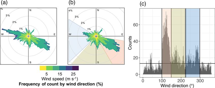
9500                                                                   J. B. Simmons et al.: Summer aerosol measurements

tor mean wind direction and mean wind speed values were            usable CN3 measurements to the period from 6 February to
calculated from the two meteorological stations and used for       the end of the voyage on 4 March.
analysis. No bias correction has been applied to correct for          Aerosol size distributions (mobility diameter) were mea-
any impact of the ship structure. The relative position of the     sured using a scanning mobility particle sizer (GRIMM nano
anemometers is forward of the ship’s superstructure and ex-        model 5.420 SMPS+C, Ainring, Bavaria, Germany). During
haust stack (Humphries et al., 2021). Therefore, it is expected    this campaign, particles between 8 and 500 nm were sized.
that when meteorological measurements may have been im-            Size distributions were measured at 5 min intervals. Compar-
pacted by the ship’s superstructure, the sampled air will carry    ison to polystyrene latex spheres showed error in size classi-
a ship exhaust signature and have hence been removed by the        fication of ≤ 5 % for particles of 81, 100, and 303 nm di-
exhaust filter described below.                                    ameter. Sample air for both aerosol number concentration
   The primary sampling inlet, which services both aerosol         and aerosol size distribution measurements was dried using
and greenhouse gas instrumentation, consists of a conic noz-       a Nafion drier (Ecotech, Melbourne, VIC, Australia) in a by-
zle with an entrance of 41.5 mm diameter, that opens up to         pass flow.
a 161.5 mm diameter stainless steel cylinder. The horizon-            Cloud condensation nuclei number concentration was
tal nozzle is actively directed into the wind with a direc-        measured using a cloud condensation nuclei counter
tional range of 300◦ . From the nozzle, the inlet bends 90◦ and    (CCN100, Droplet Measurement Technologies, Longmont,
continues down vertically for approximately 7.5 m (with two        Colorado, USA). CCN at 0.55 % supersaturation (CCN0.55 )
45◦ bends), penetrating the deck before reaching a custom-         is reported in this study. Pressure corrections were applied to
designed sampling manifold, where the sample line splits           the data, collected at 1 Hz and reported as 5 min means. The
into numerous smaller lines, a substantial bypass flow, and        sample flow was 0.5 L min−1 .
a water trap. The resulting sampling height from this setup is        222 Rn (radon) concentration was measured during the voy-

approximately 18.4 m a.s.l., depending on the ship’s draft at      age using a 700 L dual-flow-loop two-filter radon detector,
any time. The primary flow rate of the sampling line is set at     designed and built by the Australian Nuclear Science and
420 ± 15 L min−1 .                                                 Technology Organisation (Lucas Heights, NSW, Australia)
   Inlet losses have not yet been experimentally characterised     (Chambers et al., 2014; Whittlestone and Zahorowski, 1998)
for the aerosol sampling system aboard the Investigator but        with a flow rate of 65–75 L min−1 . Calibration occurs on
are a point of future work for the platform. Theoretical loss      a quasi-monthly basis through radon injections from a Py-
calculations performed for this system suggest > 95 % trans-       lon (Ottawa, ON, Canada) 222 Rn source (20.62 ± 4 % kBq
mission of 10 nm particles through this system and ∼ 75 %          226 Ra). Rn222 was measured as it can be a useful tracer of

transmission of 1 nm particles. Reported particle concentra-       terrestrial influence on air masses, particularly in the remote
tions are uncorrected and therefore represent a lower bound        marine environment, and thus provide information on the his-
on ambient aerosol population concentration. The present           tory of sampled air masses.
work includes comparison to aerosol concentrations reported           Black carbon aerosol and CO2 were also measured as
by Humphries et al. (2016) taken on board a different re-          part of the permanent instrumentation aboard the RV In-
search vessel, the Aurora Australis. It is prudent at this stage   vestigator. These measurements were only used for exhaust
to note the differing inlet efficiencies for this separate inlet   identification, and therefore these data are not presented or
system. An overall inlet transmission efficiency of 0.89 has       discussed here. Black carbon aerosol measurements were
been reported, generated from a combination of theoretical         made using a multi-angle absorption photometer (MAAP;
and experimental characterisation (Humphries et al., 2015).        model 5012, Thermo Fisher Scientific, Air Quality Instru-
   Number concentrations of in situ aerosols with diameter         ments, Franklin, MA, USA). Carbon dioxide is measured us-
greater than 3 nm (CN3 ) were measured using an ultrafine          ing a cavity ring-down spectrometer (Picarro model G2301,
condensation particle counter (UCPC, TSI Model 3776, TSI,          Picarro Inc., Santa Clara, CA, USA). Further detailed de-
Shoreview, MN, USA). Measurements were made at 10 Hz               scriptions of these measurements are available elsewhere
temporal resolution, with 1 Hz averages output by the instru-      (Humphries et al., 2021).
ment. Air was sampled at 1.5 L min−1 through the UCPC.                Significant periods of the voyage were affected by contam-
Zeros (HEPA-filtered outside air) and flow checks (external        ination of the sampled air by the ship’s exhaust due to the op-
volumetric flowmeter) were made every second day during            erational pattern of the ship. An automated exhaust removal
the voyage, with flow calibrations applied to the measure-         procedure was used on the data using an algorithm designed
ments in post-processing. A software malfunction led to in-        by Humphries et al. (2021), which identifies periods where
correct times being assigned to measurements during the first      measurements are likely to be contaminated by the ship plat-
part of the voyage. It has not proven possible to reconstruct a    form’s own exhaust and can be subsequently removed. Mea-
reliable time stamp on the early measurements, which means         surements of CN3 and CO2 that were greater than the 5 min
that they cannot be compared to other measurements or reli-        median added to 3 times the median absolute deviation or
ably filtered for the effects of the ship exhaust. This limited    those containing black carbon concentrations greater than
                                                                   0.07 ng m−3 were flagged as exhaust. Automatically filtered

Atmos. Chem. Phys., 21, 9497–9513, 2021                                             https://doi.org/10.5194/acp-21-9497-2021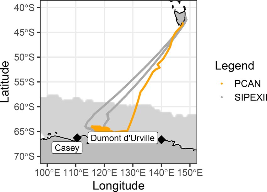
J. B. Simmons et al.: Summer aerosol measurements                                                                            9501

measurements were then manually inspected in conjunction            categories, the overall aerosol properties observed during
with black carbon and CO2 measurements for signs of con-            the voyage are presented. Differences in aerosol properties
tamination and suspect periods removed. This was done in            within categories defined by wind direction and absolute hu-
order to eliminate the influence of re-circulated, diluted ex-      midity are then considered and the implications of the find-
haust.                                                              ings discussed.
    As the exhaust filter relies on CN3 , it is not possible to
filter the data for the first part of the voyage in a manner        3.1   Categorisation by wind direction
consistent with the rest of the trip. Additionally, to ensure
no bias in a comparison of the CN3 number concentrations            Wind direction was the first variable used to categorise mea-
with the other quantities measured, it was necessary to limit       surements as it is central to the definitions of the Ferrel
this analysis to the time period of the shortest dataset, CN3       and polar cells (Aguado and Burt, 2015). Figure 2a shows
measurements as noted above (6 February until the end of the        a wind rose of all analysed measurements (6 February to
voyage).                                                            4 March). Figure 2b shows a wind rose for the period of
                                                                    the analysed measurements as in Fig. 2a, however exclud-
2.3    Back trajectory modelling                                    ing the ship’s transit back to Hobart. The boundary between
                                                                    transit measurements and other categories was selected us-
Back trajectories presented were calculated using NOAA’s            ing wind speed and latitude. Measurements taken north of
HYbrid Single Particle Lagrangian Integrated Trajectory             56.5◦ S were classified as “transit” and were associated with
(HYSPLIT) model (Draxler and Hess, 1998). The ERA-                  high wind speeds.
Interim reanalysis dataset (European Centre for Medium-                The return transit to Hobart was dominated by strong
Range Weather Forecasts, 2019) was used to produce tra-             winds from the NW (evidenced by the high density of mea-
jectories. The lack of meteorological observations at high          surements from this direction plotted in Fig. 2a), as expected
latitudes means that there is significant uncertainty in the        in the open Southern Ocean at latitudes between the seasonal
ERA datasets. A path uncertainty of 15 %–30 % of the tra-           ice zone and southern Tasmania. The aerosol characteristics
jectory travel distance has been previously estimated over the      of these open-ocean measurements differed from those ob-
Antarctic continent (Scarchilli et al., 2011). This uncertainty     served in measurements made within the seasonal ice zone.
was attributed both to the use of low-resolution meteorolog-        Transit measurements make up 15 % of the total measure-
ical data and numerical uncertainty inherent in the model.          ments plotted in Fig. 2a.
Trajectories were calculated for each hour of the voyage, in-          In the restricted wind rose (Fig. 2b), there are three areas
cluding vertical transport and limited to 72 h to minimise the      of increased measurement density, showing the prevalence
accumulation of this uncertainty. The end point was set at the      of both WNW and SE winds during the voyage. These areas
ship’s location at 20 m a.s.l. (approximate sampling height)        agree with those expected from the three-cell model of at-
for each calculation.                                               mospheric circulation. The southern edge of the Ferrel cell is
                                                                    expected to display a dominant NW wind, and the northern
2.4    Data analysis
                                                                    edge of the polar cell is expected to be associated with a dom-
Data analysis was performed in the programming language             inant SE wind (e.g. Constantin and Johnson, 2021; Laing et
“R” (R Core Team, 2017). Code used for analysis and to              al., 2011; Neiburger et al., 1971) . There also exists frequent
produce figures included in this publication can be supplied        measurements with a southerly wind, possibly linked to kata-
upon request. All measurements used for analysis were re-           batic outflow from the Antarctic continent.
sampled to 5 min time resolution. For consistency between              Measurements taken south of 56.5◦ S were then divided
figures and statistics reported in text, confidence intervals for   into 1◦ wind direction bins and a frequency histogram plot-
all reported values except in modal bin sizes were calculated       ted, presented in Fig. 2c. The frequency of wind measure-
following McGill et al. (1978), scaling the quotient of the         ments in each bin was used to create sectors of increased
interquartile range and square root of the number of observa-       measurement density. Bins which contained greater than
tions. The notch width in all box plots is also calculated using    0.2 % of total wind measurements encompassing the highest-
this method. Median concentrations are reported with 95 %           density measurement regions were selected for analysis.
confidence intervals (denoted by CI) unless noted otherwise.        Three sectors were created, associated with WNW winds
Reported r values are Pearson correlation coefficients.             and labelled Ferrel (225–298◦ , 73◦ width, n = 1444), SE
                                                                    winds labelled polar (99–148◦ , 49◦ width, n = 2211), along
                                                                    with an additional southerly sector (S, 148–217◦ , width 69◦ ,
3     Results and discussion                                        n = 1275). These sectors, shaded in Fig. 2b and c, contain
                                                                    22 %, 34 %, and 20 % of total wind measurements, respec-
In the proceeding sections, categorisation of air masses            tively. Wind direction was variable during the period of the
has been performed using both wind direction and abso-              voyage in which the ship was within the seasonal ice zone,
lute humidity. Following a definition of the borders of the         indicating periods of influence from both the Ferrel cell and

https://doi.org/10.5194/acp-21-9497-2021                                             Atmos. Chem. Phys., 21, 9497–9513, 2021
9502 J. B. Simmons et al.: Summer aerosol measurements
Figure 2. (a) Wind rose for the entire analysed PCAN voyage (6 February–4 March 2017). (b) Wind rose for wind measurements south
of 56.5◦ S (excluding measurements from the homeward transit to Hobart, Tasmania, the transit category), showing selected sectors. There
are three areas demonstrating a higher density of wind measurements, from the WNW (Ferrel, sector: 225–298◦ , width 73◦ ), from the
SE (polar, sector 99–148◦ , width 49◦ ), and from the S (southerly, 148–217◦ , width 69◦ ). These sectors, capturing 76 % of available wind
measurements, are shaded in blue (Ferrel, 22 %), khaki (southerly, 20 %), and orange (polar, 34 %) respectively. (c) Frequency histogram of
wind measurements plotted in 2b with 1◦ bin size. Ferrel (blue), southerly (khaki), and polar (orange) sectors are highlighted.
polar cells. Measurements from the southerly sector (148– 3.2 Categorisation by absolute humidity
217◦ ) have been classified separately due to the potential in-
fluence of katabatic outflow on these measurements (Cham- Using measurements from the same voyage as discussed
bers et al., 2018). These southerly data are assumed to have here, Chambers et al. (2018) found unexpected diurnal vari-
been influenced chiefly by orographic factors, and therefore ability in radon concentrations during the voyage, which was
any assumption regarding the air mass origin is difficult to explained as arising from katabatic outflow events. Events
make. Analysis of aerosol measurements from the southerly classed as katabatic outflow were associated with higher con-
sector suggests influence from both polar and Ferrel cate- centrations of CCN. A mid-morning radon minimum was es-
gories. Wind measurements not classified as Ferrel, polar, pecially indicative of this type of transport. Antarctic kata-
southerly, or transit were assigned “other”. Boxplots of these batic outflow air masses are often of free tropospheric origin
five classifications are presented in Fig. 4. (Chambers et al., 2018; Nylen et al., 2004) and are expected
A sensitivity analysis was performed on the borders of to be drier than those that have extended residence times over
the Ferrel and polar sectors, and the results of this analy- the local marine environment. Therefore, absolute humidity
sis are presented in the Supplement Table S1. Sectors were (AH) was the second meteorological variable used for cat-
shifted 10◦ closer to 360, 10◦ closer to 0◦ , symmetrically egorising aerosol measurements. Categorisations were per-
widened by 20◦ , and symmetrically narrowed by 20◦ . The formed on the same set of measurements used for division
median CN3 concentration of the selected Ferrel measure- by wind direction. Each categorisation (whether by wind or
ments is higher than or equal to each of the shifted Ferrel AH) is therefore a subset of the total voyage measurement su-
cell sectors, with all shifted sectors displaying median con- perset. Wind and AH categories overlap to differing degrees:
centrations between 229 and 265 cm−3 . The selected Ferrel a summary of overlaps is presented in Table S2.
sector median CN3 concentration is 265 (CI 252–279) cm−3 . Absolute humidity was calculated using a derivation of
Adjusting the polar cell sector introduces more variability the ideal gas law (Carnotcycle, 2012) from relative humidity
in the median CN3 concentration: adjusted sector concentra- (derived from wet- and dry-bulb temperature measurements)
tions range from 534–620 cm−3 . The median CN3 concentra- and measured ambient temperature using the following equa-
tion of the selected sector, 594 (CI 573–615) cm−3 , is in the tion, where AH is absolute humidity in units of grams per
upper region of this range. Thus, adjusting selection bound- cubic metre (g m−3 ), T is measured temperature in degrees
aries is expected to cause only small changes in the median Celsius, RH is relative humidity expressed as a percentage,
particle concentration of the Ferrel and polar cell sectors as MWH2 O is the molecular mass of water, and R is the ideal
a non-uniform particle source was being measured from a gas constant.
moving platform. The relatively small changes observed with
shifted sectors demonstrate that the median aerosol statistics
reported are robust to boundary changes in selected wind sec- 6.112e T17.67T
+243.5 × RH × MW
H2 O
tors. AH g m−3 =
(273.15 + T ) × 100 × R
Atmos. Chem. Phys., 21, 9497–9513, 2021 https://doi.org/10.5194/acp-21-9497-2021J. B. Simmons et al.: Summer aerosol measurements 9503
clean marine air dominated and that the air masses sampled
are largely free of terrestrial influence. For comparison, the
mean summer CCN0.5 concentration from the Cape Grim
“baseline” from measurements taken in the 1990s was re-
ported as 100 cm−3 (Gras, 1995). A similar summer baseline
median concentration has been reported from the site more
recently (Gras and Keywood, 2017). The Cape Grim base-
line sector is specifically selected as being free from terres-
trial and anthropogenic influence and thus can be assumed
to represent the remote Southern Ocean background signal.
The median 222 Rn concentration observed in baseline mea-
surements (2001–2008) at Cape Grim was 42 mBq m−3 (Za-
Figure 3. Frequency histogram of absolute humidity measurements horowski et al., 2013). In comparison, the non-baseline me-
including absolute humidity categories used for data analysis. The dian for the same period was 372 mBq m−3 , nearly a factor
low–mid boundary is at 4.30 gH2 O m−3 and the mid–high boundary
of 10 larger. The low concentration observed in the present
at 5.75 gH2 O m−3 . study suggests sampled air masses are free from recent ter-
restrial influence and are representative of Southern Ocean
boundary layer conditions. Overall particle number concen-
A frequency histogram, presented in Fig. 3, was constructed tration and CCN concentrations reported here are also simi-
from the time series of AH measurements. Examining the lar to those reported by Schmale et al. (2019) as CN7 (leg 1
distribution allowed three AH categories to be defined. median: 470 cm−3 ) and CCN0.2 (leg 1 median: 114 cm−3 )
These are defined in the first instance by a local minimum during the Antarctic Circumnavigation Expedition (ACE-
at 4.30 gH2 O m−3 in the frequency histogram of AH mea- SPACE), though the activation ratio observed during ACE-
surements. Measurements below this threshold were des- SPACE was lower than that observed during PCAN.
ignated as “low AH”. Measurements in the region 4.30– A median size distribution plotted from all valid SMPS
5.75 gH2 O m−3 were classified in the “mid AH” category. measurements for the analysis period during PCAN (Fig. S1)
Finally, measurements above 5.75 gH2 O m−3 were classed has a bimodal shape indicative of cloud-processed remote
in the “high AH” category. A total of 45 % (n = 3473) of marine aerosol populations (Hoppel et al., 1990), with the
valid AH measurements were classified as low AH, 39 % Hoppel minimum close to 70 nm. An Aitken mode is evi-
(n = 3028) as mid AH, and 14 % (n = 1125) as high AH. dent, centred at 38.5 nm. A less concentrated accumulation
The low AH category is expected to capture air masses with mode centred at 126 nm is also present. This distribution is
either a katabatic flow or free-tropospheric source region as similar to that observed in marine polar air masses during a
air from these sources has not had an extended residence time summer voyage close the Antarctic peninsula (Fossum et al.,
in a marine environment. The mid AH is expected to consist 2018), though smaller in magnitude.
largely of marine air masses. Note that the high AH category Previous aerosol number concentration measurements in
overlaps almost exclusively (> 99 %) with the transit cate- the East Antarctic seasonal ice zone suggested the influ-
gory as defined above. This overlap is expected for maritime ence of large-scale atmospheric transport on locally observed
measurements as the water saturation pressure is dependent aerosol concentrations (e.g. Humphries et al., 2021; Al-
on temperature and ambient temperature increase during the roe et al., 2020). In these PCAN measurements, immediate
transit from the Antarctic coast to Tasmania. changes in aerosol number concentration suggestive of an at-
mospheric boundary at the polar front, measured as CN3 or
3.3 General properties of observed aerosol populations CCN0.55 , were not observed to the extent of previous cam-
paigns in the region (Alroe et al., 2020; Humphries et al.,
Measurements were made for the entire voyage, but as noted 2016). It must be considered at this point that the polar front
above an instrument malfunction meant CN3 measurements describes a feature of climatological atmospheric circulation,
are not available until 6 February 2017. For the period where which is influenced on a shorter timescale by meteorological
all measurements are available, the data have been sum- conditions. Therefore the strength of this atmospheric bound-
marised as boxplots (Fig. 4a, b, and c present boxplots of ary is expected to vary over the synoptic timescale. Mete-
CN3 , CCN0.55 , and 222 Rn). The median CCN0.55 concen- orological variables have been used to place aerosol mea-
tration of 167 (CI 158–176) cm−3 implies approximately surements into the framework of the polar and Ferrel (mid-
half the particles measured as CN3 could be activated as latitude) cells.
CCN (concentration of 354 (CI 344–363) cm−3 ). The me-
dian 222 Rn concentration observed during the voyage was
64.5 (CI 62–67) mBq m−3 . The low concentrations of both
aerosol number and 222 Rn suggest that measurements of
https://doi.org/10.5194/acp-21-9497-2021 Atmos. Chem. Phys., 21, 9497–9513, 20219504 J. B. Simmons et al.: Summer aerosol measurements
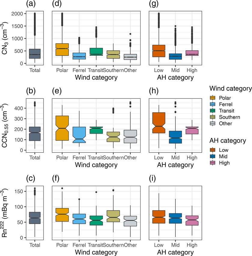
Figure 4. Box plots for all analysed measurements and divided by category for (a), (d), and (g) CN3 ; (b), (e), and (h) CCN0.55 ; and (c),
(f), and (i) Rn222 . Plots in the centre column are split by wind category, and plots in the right-hand column are split by absolute humidity.
Notches indicate the 95 % confidence intervals in the median. Black dots represent outliers, defined as points greater than 1.5 times the
interquartile ranges distant from the nearest quartile. Medians and confidence intervals for each variable in each category are reported in
Table S3.
3.4 Aerosol variables and radon grouped by wind nental and anthropogenic aerosol sources on boundary layer
direction aerosol populations in the northern latitudes of the Southern
Ocean, particularly above 50◦ S, as reported by Humphries et
Figure 4 presents box plots of CN3 (Fig. 4d), CCN0.55 al. (2021). Measurements reported here as Ferrel cells were
(Fig. 4e), and radon concentrations (Fig. 4f) grouped by wind taken too far south to be significantly influenced by these ad-
direction. Statistics represented graphically in Fig. 4 are also ditional particle sources.
presented in tabular form in Table S2. In each case the me- In the southern sector the median CN3 concentration is
dian concentration is higher in polar cell measurements than 354 (CI 329–379) cm−3 , between those observed in the polar
in Ferrel cell measurements. Median CN3 concentration in and the Ferrel. As discussed in Sect. 3.1, southern measure-
the polar cell, 594 (CI 573–615) cm−3 , is approximately a ments are separated from the polar–Ferrel classification in an
factor of 2 larger than the Ferrel cell median, at 263 (CI 250– attempt to isolate the known influence of katabatic outflow
277) cm−3 . Median CCN0.55 concentrations in the polar cell on near-coast measurements of boundary layer aerosol in the
were 208 (CI 176–240) cm−3 , compared to a median con- East Antarctic seasonal ice zone (Chambers at el., 2018). It
centration of 113 (CI 84–142) cm−3 in the Ferrel cell. Me- is recognised that identifying katabatic flow by wind direc-
dian radon concentration in the polar cell was 78.3 (CI 73.3– tion is not ideal. However, given the context of classifying
83.3) mBq m−3 compared to 59.1 (CI 54.3–63.9) mBq m−3 measurements by wind direction, this method has been used
in the Ferrel cell. For both aerosol variables, the transit cat- in this study for consistency. The remaining 24 % of mea-
egory median is between those observed in the polar and surements of uncertain air mass history, classified as “other”,
Ferrel (Fig. 4). The higher median concentrations of CN3 have a mean CN3 concentration of 250 (CI 240–250) cm−3 .
and CCN0.55 observed in the transit category (compared to This is the lowest median CN3 concentration observed in any
the Ferrel) are likely due to the increased influence of conti- category. The lowest median 222 Rn concentration was also
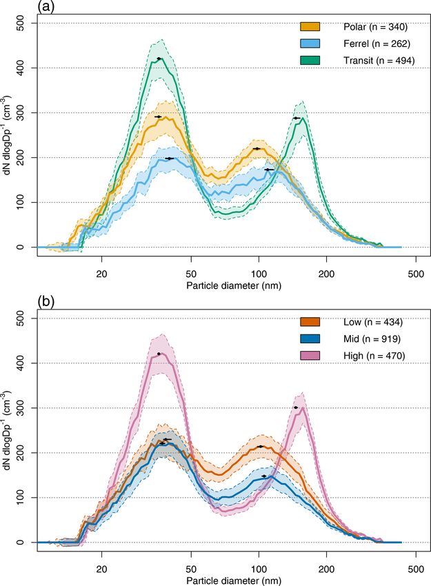
Atmos. Chem. Phys., 21, 9497–9513, 2021 https://doi.org/10.5194/acp-21-9497-2021J. B. Simmons et al.: Summer aerosol measurements 9505 observed in the “other” classification, suggesting air masses polar distribution. This information, coupled with the more sampled may have sources in the remote atmosphere distant concentrated accumulation mode observed by Schmale et from aerosol precursor sources and continental influence. al. (2019), suggests the particle populations observed during Median aerosol size distributions divided by wind sector PCAN may have different air mass histories than those ob- are presented in Fig. 5a. Each category displays a bimodal served in the West Antarctic. There is evidence for differing distribution. The transit distribution is the most strongly bi- aerosol regimes near the East and West Antarctic coasts in modal. This is indicative of heavily cloud-processed marine the differences in observed particle concentrations and acti- aerosol (Hoppel et al., 1990) and results in one modal max- vation ratios during the 2016–2017 austral summer (Schmale imum in the Aitken mode (37.2 nm) and the other in the ac- et al., 2019). cumulation mode (157 nm). The median magnitudes of the To further characterise the observed size distributions, the modes are 421 (CI 378–464) and 288 (CI 251–326) cm−3 re- modal sizes were determined. That is, the size bin with the spectively (Fig. 5a). highest median concentration in the Aitken and accumulation In contrast, the distributions plotted for the Ferrel and po- size range is selected as the mode. To estimate the uncertainty lar cells differ from the transit period distribution. Both po- in the modal particle size for Aitken- and accumulation-mode lar and Ferrel distributions contain two local maxima with aerosol, the bin with maximum concentration was retrieved a smaller degree of bimodality. It should be noted that all from each individual distribution and analysed. Details of aerosol populations, even those potentially descending from this analysis are found in the Supplement Sect. S1. These the free troposphere, had the potential to be cloud-processed results, summarised in Table S4, are different to the modal before sampling. Thus, the observed bimodality in all cate- bin sizes retrieved for the overall median distributions noted gories is not surprising. The polar air mass has a higher par- above. This is a result of the distributions changing as con- ticle concentration across the distribution than the Ferrel (as centrations change. While significant differences between expected accounting for the larger median CN3 concentra- the modal size bins do exist between categories when calcu- tion). The difference is relatively uniform across the distribu- lating the uncertainty using this method, these differences are tion between 20 and 120 nm. The polar and Ferrel distribu- small in magnitude (less than 12 nm in each mode between tions have modes in similar size ranges: the smaller mode in polar and Ferrel and between low and mid AH) for both wind the polar cell has a maximum at 38.5 and at 40 nm in the Fer- and AH categorisations. It is therefore unclear what conclu- rel. The larger mode is at a slightly larger diameter in the Fer- sions can be drawn from this result. The median modes of rel cell dataset (109 nm) than the polar cell (101 nm). Modal individual distributions are plotted with 95 % CI for each cat- sizes and concentrations from Fig. 5 are summarised in Table egory in Fig. 5. S3. Higher particle concentrations in the polar cell have 3.5 Aerosol variables and radon grouped by absolute been observed previously in the East Antarctic seasonal ice humidity zone. In addition to the spring 2012 campaign SIPEXII (Humphries et al., 2016) and identification of katabatic in- The categorisation by absolute humidity should allow for fluence on local CCN concentration (Chambers et al., 2018) identification of the impact of katabatic outflow on the referred to previously, there is evidence for a change in aerosol population. Figure 4 displays boxplots of CN3 , aerosol population across the polar front during a summer CCN0.55 , and radon concentrations grouped by absolute hu- latitudinal transect of the Southern Ocean in 2016 (Alroe et midity category. Measurements of CN3 and CCN0.55 in the al., 2020), along with variability in the Aitken mode depen- low AH category are higher than those in the mid and high dant on marine biological precursors and synoptic-scale sys- AH categories. Median CN3 and CCN0.55 concentrations in tems. Accumulation-mode peaks in both the Ferrel and polar the low AH category were 507 (CI 489–526) cm−3 and 228 median size distributions are less concentrated than in the (CI 201–255) cm−3 respectively. In comparison, the mid AH Aitken mode. medians for CN3 and CCN0.55 were 284 (CI 276–292) cm−3 These particle concentration characteristics contrast with and 117 (CI 107–128) cm−3 , respectively. This is consis- observations made by Schmale et al. (2019) in the West tent with the finding that katabatic outflow events are asso- Antarctic sector of the Southern Ocean. Using k-means clus- ciated with higher aerosol concentrations than locally sam- tering, they observed two clusters of aerosol size distribution pled air masses observed by Chambers et al. (2018), as kata- clusters with different air mass histories. Cluster 1 was in- batic outflow events are likely included in the low AH cate- dicative of extended residence in the Southern Ocean ma- gory due to the dry nature of katabatic air masses. While not rine boundary layer (similar to the Ferrel category identi- statistically significant, a difference in radon concentration fied here), while the other, cluster 2, showed influence of is also noted between the categories: a median of 68.1 (CI descent over the Antarctic continent and polynya regions. 64.0–72.1) mBq m−3 in during low AH compared to 63.6 (CI The modal sizes of cluster 1 distribution are larger than those 60.3–66.9) mBq m−3 during mid AH. It is likely that the low observed in the present Ferrel measurements. The same is AH category captures the katabatic outflow present in type true when comparing the cluster 2 distribution to the present 3 and type 4 days presented in Chambers et al. (2018). Type https://doi.org/10.5194/acp-21-9497-2021 Atmos. Chem. Phys., 21, 9497–9513, 2021
9506                                                                         J. B. Simmons et al.: Summer aerosol measurements

                                                                       shows bimodal character. The low AH and mid AH have a
                                                                       smaller magnitude of bimodality as there is a smaller con-
                                                                       centration difference between modes and the Hoppel mini-
                                                                       mum compared to the transit distribution. The smaller mode
                                                                       in each of these distributions, in the Aitken range, is similar
                                                                       in magnitude and concentration: at 38.5 nm with a concen-
                                                                       tration of 230 (CI 193–266) cm−3 in low AH and at 40.0 nm
                                                                       a concentration of 221 (CI 194–249) cm−3 in mid AH. The
                                                                       larger mode is more concentrated in the low AH category,
                                                                       with a concentration of 214 (CI 189–240) cm−3 at 106 nm,
                                                                       than the mid AH: a concentration of 148 (CI 125–171) cm−3
                                                                       at 113 nm. The significance of the results presented above
                                                                       will be discussed in the following paragraphs.

                                                                       3.6   Evidence for large-scale atmospheric transport
                                                                             influence on Southern Ocean aerosol populations

                                                                       Differences in CN3 and CCN0.55 concentration are evident
                                                                       when meteorological variables are used to group aerosol
                                                                       measurements. Grouping measurements by wind direction
                                                                       produces higher median concentrations of CN3 and CCN
                                                                       sampled during wind directions indicative of polar cell air.
                                                                       Similarly, higher concentrations of CN3 and CCN0.55 were
                                                                       observed when AH is less than 4.3 gH2 O m−3 . The southerly
                                                                       and polar cell air is expected to be drier than Ferrel cell
                                                                       air (which has a theoretically longer residence time in the
                                                                       marine boundary layer as well as having increased contact
                                                                       with warmer ocean water). These results provide evidence
Figure 5. Median particle size distributions for (a) each wind cat-    that large-scale atmospheric transport (i.e. the atmospheric
egory and (b) each AH category. Shaded areas represent the 95 %        transport included in the polar and Ferrel cells) influences
confidence interval in the median for each bin size. Note the diame-
                                                                       local aerosol populations in the East Antarctic seasonal ice
ter axis is logarithmic in scale. The modal sizes and concentrations
for each distribution are reported in Table S3. Black points plotted
                                                                       zone. Note, however, that the aerosol size distributions sam-
on each distribution indicate the median Aitken and accumulation       pled under different wind and AH regimes are similar. The
mode generated from analysis of individual size distributions. Error   aerosol size distributions are also similar between polar and
bars represent the 95 % confidence interval. More detail is provided   Ferrel wind measurements. The similarity between these me-
in the Supplement Sect. S1 and Table S4.                               dian size distributions, as depicted in Fig. 5, suggests that a
                                                                       common aerosol source may contribute to these populations.
                                                                          Back trajectory analysis can be used to further identify
4 days were defined by Chambers et al. (2018) using a mid-             influence of large-scale atmospheric processes on boundary
morning Rn222 minimum, daytime winds from the S/SW, and                layer aerosol in the East Antarctic seasonal ice zone. HYS-
relatively strong winds, indicative of air masses strongly in-         PLIT back trajectories were run for each hour, on the hour, of
fluenced by katabatic outflow. Type 3 days shared similar              the voyage. The ship’s location at each time was used as the
characteristics to type 4 days, though to a lesser extent. The         trajectory end point. Trajectories were separated into wind
median CCN0.55 concentration observed in the present anal-             and absolute humidity categories using a similar method to
ysis for low AH agrees well with maximum CCN concen-                   that used for the aerosol measurements. The classification
trations reported for mid-morning katabatic outflow (type 3            category for the wind direction or AH at the trajectory end-
and 4 days) CCN peaks (Chambers et al., 2018). It should be            point was used to classify the trajectory. Median vertical pro-
noted that the low AH category includes a greater percentage           files, frequency histograms, and trajectory maps for each cat-
of the measurements (45 %) compared to the type 3 and 4                egory were constructed and are presented in Figs. S2 and S3.
days reported by Chambers et al. (2018) (∼ 27 %) so likely                Distinct air mass histories are expected to contribute to
includes measurements not influenced by katabatic drainage.            different aerosol population characteristics observed in each
   Median size distributions plotted for each AH category are          classification. Back trajectory analysis suggests a greater free
presented in Fig. 5b. As noted earlier, the high AH category           tropospheric influence is present in the polar wind cate-
is also the transit category and hence a measurement of open-          gory compared to the Ferrel wind category. The boundary
ocean Ferrel cell aerosol. Similar to Fig. 5a, each distribution       layer height in this region of the Southern Ocean has been

Atmos. Chem. Phys., 21, 9497–9513, 2021                                                  https://doi.org/10.5194/acp-21-9497-2021
J. B. Simmons et al.: Summer aerosol measurements 9507
measured to be 900 ± 400 m north of the polar front and PCAN. The magnitude of the change between the polar and
700 ± 200 m south of the polar front during summer and Ferrel cell during SIPEXII was a factor of approximately 4,
early autumn voyages (Alexander and Protat, 2019). The me- whereas for PCAN this change is closer to a factor of 2.
dian profile for the polar category shows air masses residing It is important to note that these measurements were taken
above 1000 m a.g.l. 48 h before the trajectory endpoint. Sam- from different platforms, and therefore different particle in-
pled air masses in the polar category are therefore likely to let transmission efficiencies must be considered. However,
have significant free-tropospheric influence. The median pro- the difference in the magnitude of enhancement observed in
files for the Ferrel and transit wind categories show no such the polar cell, which does not depend on inlet transmission
development, instead keeping close to the surface for the du- efficiency in both voyages, demonstrates that there is a robust
ration of the 72 h modelled (Fig. S2). The large interquartile difference in aerosol populations observed between voyages.
ranges on this plot reflect significant variability in air mass A further difference between spring and summer measure-
altitude. Interestingly, the trajectories for the southerly cate- ments becomes evident when considering the size of particle
gory also show history of descending air masses. populations measured during the voyages. The Ferrel–polar
A similar result is generated when examining trajectories cell transition during SIPEXII was especially prominent in
grouped by AH category. The mid and high AH category me- the CN3−10 fraction, with the median CN3−10 concentration
dian trajectory vertical profiles show little vertical develop- in the Ferrel cell reported at 45 cm−3 compared to a median
ment in the 72 h prior to measurement (Fig. S3). In contrast, of 776 cm−3 in the polar cell. This is attributed to a change
the low AH category median vertical profile demonstrates of aerosol source by Humphries et al. (2016). A lack of a
vertical development comparable to that of the polar wind CN10 measurement on board during PCAN (due to instru-
category, with significant residence time at free-tropospheric ment malfunctions) prevents a direct comparison of this met-
altitudes in the 72 h prior to sampling. ric between voyages. Aerosol size distribution measurements
Back trajectories indicate a greater free tropospheric in- from PCAN can be used however: the SMPS instrument used
fluence on air masses sampled under polar wind regimes on this voyage observed measurements as small as 8 nm di-
and with low AH than during other measurement periods. ameter during the voyage, allowing the particle concentration
Higher particle counts (CN3 and CCN0.55 ) are also observed to be calculated in the CN3−8 range. During PCAN, the me-
in these air masses. Observation of higher aerosol num- dian CN3−8 concentration in the Ferrel cell was 118 cm−3 ,
ber concentrations and a free tropospheric influence on air compared to 148 cm−3 in the polar cell. This suggests the
masses sampled in the polar cell in the East Antarctic sea- difference in aerosol number concentration observed during
sonal ice zone are common to the summer measurements PCAN is not driven by a large change in concentration of
presented here and the spring 2012 measurements reported very small particles as observed during SIPEXII.
in Humphries et al. (2016). However, there are some key dif- Polar cell measurements from SIPEXII and PCAN (de-
ferences between measurements, suggesting different source fined by wind direction) were compared to investigate this
and air mass transport mechanisms. further. Figure 6 displays four correlation plots: AH measure-
ments and atmospheric pressure measurements from PCAN
3.7 Evidence for seasonality in seasonal ice zone (top row) and SIPEXII (bottom row) are plotted against CN3
regional aerosol sources measurements. Events of anomalously high CN3 concentra-
tion during SIPEXII as identified by Humphries et al. (2016)
Comparing SIPEXII polar cell aerosol measurements from are excluded from this analysis. CN3 shows a negative rela-
spring 2012 to the PCAN polar measurements (classified by tionship with absolute humidity in PCAN polar cell measure-
wind direction) indicates there may be different sources, or ments (r = −0.50). This relationship is weaker for SIPEXII
source strengths, for aerosol populations observed in spring measurements (r = −0.26). In contrast, a negative relation-
and summer despite some similar characteristics. Humphries ship is observed between SIPEXII polar cell CN3 measure-
et al. (2016) defined polar cell measurements using a clear ments and atmospheric pressure (r = −0.61), discussed in
change in observed aerosol population along with detailed detail in Humphries et al. (2016). This relationship is weaker
back trajectory analysis. This method is different to that used in the PCAN polar cell measurements (r = −0.23). This sug-
here. However, the persistent nature of dominant surface gests the source regions or mechanisms of measured polar
winds associated with polar and Ferrel cells, coupled with cell aerosol in the East Antarctic seasonal ice zone may vary
back trajectories (plotted in Figs. S2 and S3) aligning with between seasons. A free tropospheric injection model pre-
those modelled for SIPEXII measurements, allows compari- sented by Humphries et al. (2016), associated with events
son between polar cell measurements to be made between the of local low atmospheric pressure, was used to account for
voyages. The median CN3 concentration in the polar cell dur- unexpectedly high concentrations of small aerosol during
ing SIPEXII was 816 cm−3 (Humphries et al., 2016), com- SIPEXII. This tropospheric injection may not be the dom-
pared to a median polar CN3 concentration of 594 cm−3 re- inant source of polar cell aerosol measured during summer
ported here. The median SIPEXII Ferrel cell concentration 2017. This conclusion was also drawn from the analysis
was 196 cm−3 , compared to a median of 263 cm−3 during of radon diurnal cycles and CCN concentrations from the
https://doi.org/10.5194/acp-21-9497-2021 Atmos. Chem. Phys., 21, 9497–9513, 2021You can also read