CE-DYNAM (v1): a spatially explicit process-based carbon erosion scheme for use in Earth system models - Geosci. Model Dev.
←
→
Page content transcription
If your browser does not render page correctly, please read the page content below
Geosci. Model Dev., 13, 1201–1222, 2020
https://doi.org/10.5194/gmd-13-1201-2020
© Author(s) 2020. This work is distributed under
the Creative Commons Attribution 4.0 License.

CE-DYNAM (v1): a spatially explicit process-based carbon erosion
scheme for use in Earth system models
Victoria Naipal1,2 , Ronny Lauerwald3 , Philippe Ciais1 , Bertrand Guenet1 , and Yilong Wang1
1 Laboratoiredes Sciences du Climat et de l’Environnement, CEA CNRS UVSQ, Gif-sur-Yvette, France
2 Ludwig Maximilian University of Munich, Munich, Germany
3 Department of Geoscience, Environment and Society, Université Libre de Bruxelles, Brussels, Belgium

Correspondence: Victoria Naipal (vnaipal24@gmail.com)

Received: 18 April 2019 – Discussion started: 11 June 2019
Revised: 23 January 2020 – Accepted: 7 February 2020 – Published: 17 March 2020

Abstract. Soil erosion by rainfall and runoff is an impor-       over long timescales, and (3) its compatibility with global
tant process behind the redistribution of soil organic carbon    land surface models, thereby providing opportunities to study
(SOC) over land, thereby impacting the exchange of carbon        the effect of soil erosion under global changes.
(C) between land, atmosphere, and rivers. However, the net           We present the model structure, concepts, limitations, and
role of soil erosion in the global C cycle is still unclear as   evaluation at the scale of the Rhine catchment for the period
it involves small-scale SOC removal, transport, and rede-        1850–2005 CE (Common Era). Model results are validated
position processes that can only be addressed over selected      against independent estimates of gross and net soil and C
small regions with complex models and measurements. This         erosion rates and the spatial variability of SOC stocks from
leads to uncertainties in future projections of SOC stocks and   high-resolution modeling studies and observational datasets.
complicates the evaluation of strategies to mitigate climate     We show that despite local differences, the resulting soil and
change through increased SOC sequestration.                      C erosion rates, as well as SOC stocks from CE-DYNAM,
   In this study we present the parsimonious process-based       are comparable to high-resolution estimates and observations
Carbon Erosion DYNAMics model (CE-DYNAM) that links              at subbasin level.
sediment dynamics resulting from water erosion with the C            We find that soil erosion mobilized around 66 ± 28 Tg
cycle along a cascade of hillslopes, floodplains, and rivers.    (1012 g) of C under changing climate and land use over the
The model simulates horizontal soil and C transfers triggered    non-Alpine region of the Rhine catchment over the entire pe-
by erosion across landscapes and the resulting changes in        riod, assuming that the erosion loop of the C cycle was nearly
land–atmosphere CO2 fluxes at a resolution of about 8 km         steady state by 1850. This caused a net C sink equal to 2.1 %–
at the catchment scale. CE-DYNAM is the result of the cou-       2.7 % of the net primary productivity of the non-Alpine re-
pling of a previously developed coarse-resolution sediment       gion over 1850–2005 CE. This sink is a result of the dynamic
budget model and the ecosystem C cycle and erosion removal       replacement of C on eroding sites that increases in this period
model derived from the Organising Carbon and Hydrology           due to rising atmospheric CO2 concentrations enhancing the
In Dynamic Ecosystems (ORCHIDEE) land surface model.             litter C input to the soil from primary production.
CE-DYNAM is driven by spatially explicit historical land use
change, climate forcing, and global atmospheric CO2 con-
centrations, affecting ecosystem productivity, erosion rates,
and residence times of sediment and C in deposition sites.       1   Introduction
The main features of CE-DYNAM are (1) the spatially ex-
plicit simulation of sediment and C fluxes linking hillslopes    Soils contain more carbon (C) than the atmosphere and liv-
and floodplains, (2) the relatively low number of parameters     ing biomass together. Relatively small disturbances (anthro-
that allow for running the model at large spatial scales and     pogenic or natural) to soil C pools over large areas could add
                                                                 up to substantial C emissions (Ciais et al., 2013). With the

Published by Copernicus Publications on behalf of the European Geosciences Union.
1202                                                                                         V. Naipal et al.: CE-DYNAM (v1)

removal of natural vegetation and the introduction of mecha-        uncertainties in lateral C fluxes between land and ocean for
nized agriculture, humans have accelerated soil erosion rates.      past and future scenarios estimated by global empirical mod-
Over the last 2 to 3 decades, studies have shown that wa-           els on riverine C export (Ludwig and Probst, 1998; Mayorga
ter erosion (soil erosion by rainfall and runoff) amplified by      et al., 2010).
human activities has substantially impacted the terrestrial C          To address these knowledge gaps, we present a parsi-
budget (Doetterl et al., 2012; Lal, 2003; Lugato et al., 2018;      monious process-based Carbon Erosion DYNAMics model
Van Oost et al., 2007, 2012; Stallard, 1998; Wang et al., 2017;     (CE-DYNAM), which integrates sediment dynamics result-
Tan et al., 2020; Chappell et al., 2016). However, the net ef-      ing from water erosion with the SOC dynamics at the re-
fect of water erosion on the C cycle at the regional-to-global      gional scale. The SOC dynamics are calculated consistently
scale is still under debate. This leads to uncertainties in the     with drivers of land use change, CO2 , and climate change
future projections of the soil organic C (SOC) reservoir, and       by a process-based global land surface model (LSM), with a
it complicates the evaluation of strategies to mitigate climate     simplified reconstruction of the last century increase of crop
change by increased SOC sequestration.                              productivity. This modeling approach consists of a global
   The study of Stallard (1998) was one of the first to show        sediment budget model coupled to the SOC removal, in-
that water erosion not only leads to additional C emissions         put, and decomposition processes diagnosed from the OR-
but also sequesters C due to the photosynthetic replace-            CHIDEE global LSM in an offline setting (Naipal et al.,
ment of SOC at eroding sites and the stabilization of SOC           2018). The main aim of our study is to quantify the hori-
in deeper layers at burial sites. The study by Van Oost et          zontal transport of sediment and C along the continuum of
al. (2007) was the first to confirm the importance of the se-       hillslopes and floodplains and at the same time analyze its
questration of SOC by agricultural erosion at a global scale        impacts on the land–atmosphere C exchange. We validate the
using isotope tracers. Wang et al. (2017) gathered data on          new model with regional observations and high-resolution
SOC profiles from erosion and deposition sites around the           modeling results of the Rhine catchment. It should be noted
world and confirmed that water erosion on agricultural land         here that the structure of CE-DYNAM is designed in a way
that started from the early-to-middle Holocene has caused           that the model can be adapted easily to other large catch-
a large net global land C sink. Other studies, however, ar-         ments after calibrating the model parameters to the specific
gue that soil erosion is a net C source to the atmosphere           environmental conditions in those catchments. We also dis-
due to increased SOC decomposition following soil aggre-            cuss the model uncertainties and the sensitivity of the model
gate breakdown during transport and at deposition sites (Lal,       to changes in key model parameters and assumptions made.
2003; Lugato et al., 2018). Most studies modeling soil ero-         In the next sections we give a detailed overview of the CE-
sion and its net effect on SOC dynamics at the global scale,        DYNAM model structure; the coupling of erosion, deposi-
however, do not account for the full range of complex ef-           tion, and transport with the coarse-resolution SOC dynam-
fects of climate change, CO2 -driven increase in productiv-         ics of ORCHIDEE; model application and validation for the
ity and potentially soil C inputs, harvest of biomass, land use     non-Alpine region of the Rhine catchment; and its potential
change, and changes in cropland management (Borrelli et al.,        and limitations.
2018; Doetterl et al., 2012; Chappell et al., 2016; Lugato et
al., 2018; Van Oost et al., 2007; Wang et al., 2017). In ad-
dition, models used at large spatial scales mainly focus on         2     Methods
hillslopes and removal processes and neglect floodplain sed-
                                                                    2.1    General model description
iment and SOC dynamics (Borrelli et al., 2018; Chappell et
al., 2016; Lugato et al., 2018; Van Oost et al., 2007; Tan et       CE-DYNAM version 1 (v1) is the result of coupling a large-
al., 2020). This can lead to substantial biases in the assess-      scale erosion and sediment budget model (Naipal et al.,
ment of net effects of SOC erosion at the catchment scale as        2016) with the SOC scheme of the ORCHIDEE LSM (Krin-
floodplains can store substantial amounts of sediment and C         ner et al., 2005). The most important features of the model
(Berhe et al., 2007; Hoffmann et al., 2013a, b). Studies ad-        are (1) the spatially explicit simulation of lateral sediment
dressing long-term large-scale sediment yield from hillslopes       and C transport fluxes over land, linking hillslopes and flood-
and floodplains, such as Pelletier (2012), do not explicitly ac-    plains; (2) the consistent simulation of vertical C fluxes cou-
count for the redistribution of sediment and SOC over land.         pled with horizontal transport; (3) the low number of param-
   Furthermore, soil erosion is one of the main contributors        eters compared to other C erosion models that operate at a
to particulate organic carbon (POC) fluxes in rivers and C          high spatial resolution (Lugato et al., 2018; Billings et al.,
export to the coastal ocean. The riverine POC fluxes are usu-       2019), which allows for running the model at large spatial
ally much smaller than the SOC erosion fluxes, due to de-           scales and over long timescales up to several thousands of
composition and burial in floodplains and in benthic sedi-          years; (4) the generic input fields for application to any re-
ments, while POC losses occur in the river network (Tan et          gion or catchment; and (5) the compatibility with the model-
al., 2017; Galy et al., 2015). Therefore, uncertainties in large-   ing structure of LSMs.
scale SOC erosion rates over land will lead to even larger

Geosci. Model Dev., 13, 1201–1222, 2020                                              www.geosci-model-dev.net/13/1201/2020/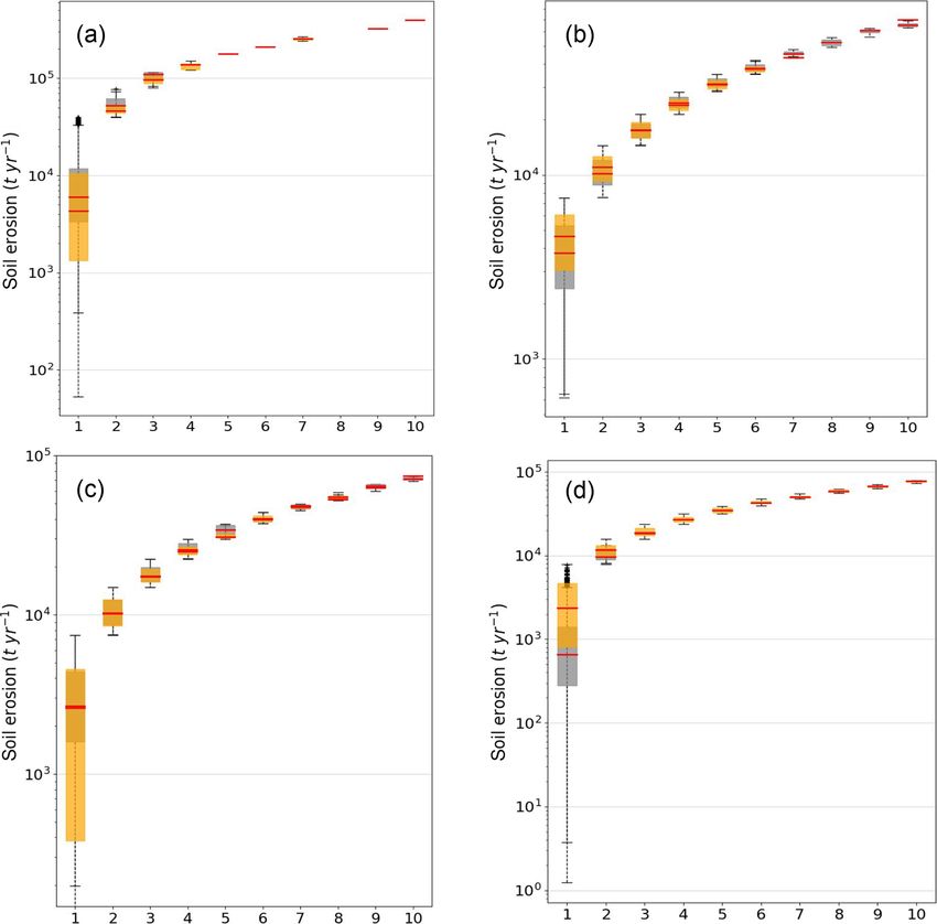
V. Naipal et al.: CE-DYNAM (v1)                                                                                                1203

   In the ORCHIDEE LSM, terrestrial C is represented by
eight biomass pools: four litter pools and three SOC pools.
Each of the pools varies in space, time, and over the 12 plant
functional types (PFTs). An extra PFT is used to represent
bare soil. Anthropogenic and natural disturbances (as a re-
sult of climatic changes) to the C pools include fire, crop
harvest, changes to the gross primary productivity (GPP), lit-
terfall, and autotrophic and heterotrophic respiration (Krin-
ner et al., 2005; Guimberteau et al., 2018). The C-cycle pro-
cesses are represented by a C emulator that reproduces for
each PFT all C pools and fluxes between the pools exactly
as in ORCHIDEE in the absence of erosion. A net land
use change scheme is included in the emulator with mass-
conservative bookkeeping of SOC and C input when a PFT
is changed into another PFT from anthropogenic land use
change (Naipal et al., 2018). The sediment budget model
has been added in the emulator to simulate large-scale long-
term soil and SOC redistribution by water erosion using
coarse-resolution precipitation, land-cover, and leaf area in-
dex (LAI) data from Earth system models (Naipal et al.,
2015, 2016). The C emulator including erosion removal was
developed by Naipal et al. (2018) to reproduce the SOC ver-        Figure 1. A conceptual diagram of CE-DYNAM. The red arrows
tical profile, removal of soil and SOC, and compensatory           represent the C fluxes between the C pools and reservoirs, while
SOC storage from litter input. As soil erosion is assumed to       the black arrows represent the links between the erosion processes
not change soil and hydraulic parameters but only the SOC          (removal, deposition, and transport).
dynamics, the emulator allows for substituting of the OR-
CHIDEE model and performing simulations on timescales
                                                                   their quantification still includes many uncertainties and is
of millennia with a daily time step and a spatial resolution
                                                                   not practical for applications at regional to global scales.
of 5 arcmin (∼ 8 km × 8 km), which would be a very compu-
                                                                   These factors are largely affected by local artificial structures
tationally expensive or nearly impossible with the full LSM.
                                                                   (such as field size) and management practices, which are dif-
The concept and all equations of the emulator are described
                                                                   ficult to assess for the present day and whose changes over
in Naipal et al. (2018). The following subsections describe
                                                                   the past are even more uncertain. In addition, we focus in this
the different components of CE-DYNAM that couple the C
                                                                   study on the potential effect of soil erosion on the C budget
and soil removal scheme (Naipal et al., 2018) with the hor-
                                                                   without erosion-control (EC) practices.
izontal transport and burial of eroded soil and C (Naipal et
                                                                      Naipal et al. (2015) have developed a methodology to de-
al., 2016).
                                                                   rive the S and R factors from 5 arcmin resolution (5 arcmin×
2.2   The soil erosion scheme                                      5 arcmin raster) data on elevation and precipitation, while at
                                                                   the same time preserving the high-resolution spatial variabil-
The potential gross soil erosion rates are calculated by           ity in slope and temporal variability in erosivity. In the rest of
the Adjusted Revised Universal Soil Loss Equation (Adj.            the paper we will refer to X km (or arcmin) by X km (or ar-
RUSLE) model (Naipal et al., 2015), which is based on the          cmin) raster cells always with X km (or arcmin) resolution.
Revised Universal Soil Loss Equation (RUSLE) (Renard et            Despite the comparatively coarse resolution of the erosion
al., 1997) and is part of the sediment budget model (Naipal        model, the so-derived R factor was shown to compare well
et al., 2016) (Fig. 1). In the Adj. RUSLE the yearly-average       with the corresponding high-resolution product published by
soil erosion rate is a product of rainfall erosivity (R), slope    Panagos et al. (2017). In the study by Naipal et al. (2016),
steepness (S), land cover and management (Cm), and soil            where the soil erosion model was applied for the last mil-
erodibility (K):                                                   lennium, the change in climate was taken into account in the
                                                                   calculation of the R factor. For this study, we assume that
E = S × R × K × Cm.                                         (1)    the climate zones as defined by the Köppen–Geiger climate
                                                                   classification have not changed drastically since 1850 CE.
Note that the original RUSLE model further includes a slope-
length factor (L), which gives the length of a field in the di-
rection of steepest descent, and a support practice factor (P ),
which accounts for management practices to mitigate soil
erosion. These two factors have been excluded here, because

www.geosci-model-dev.net/13/1201/2020/                                                Geosci. Model Dev., 13, 1201–1222, 2020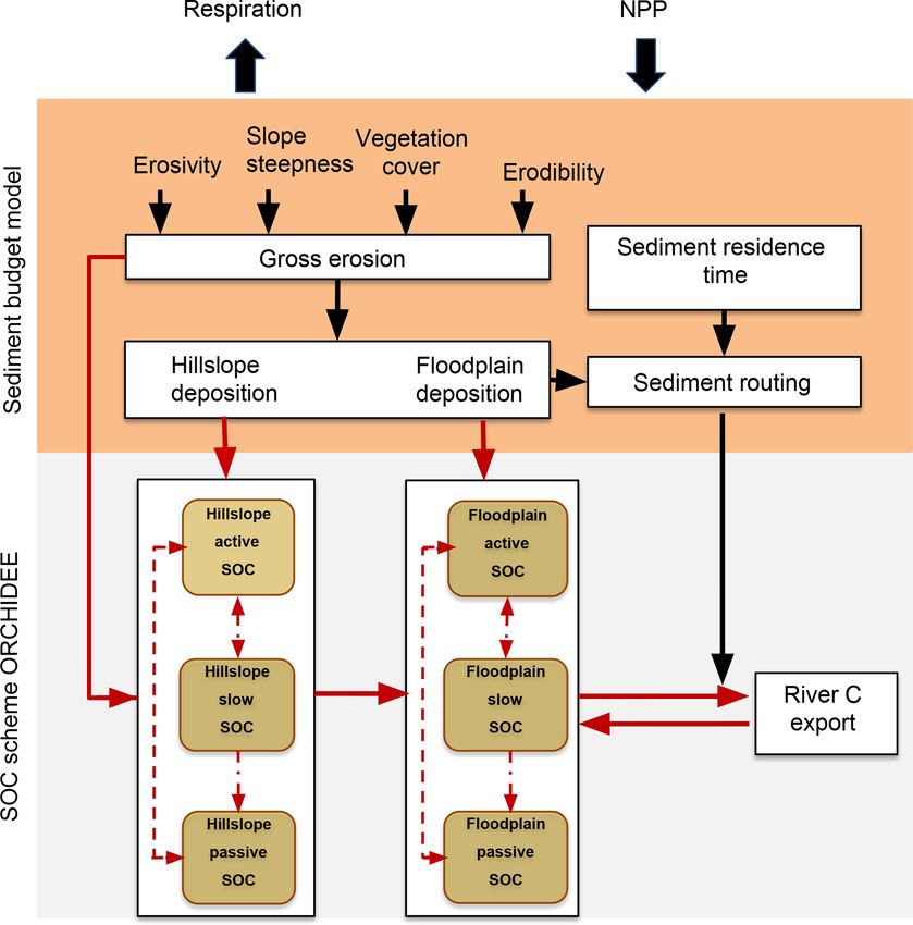
1204                                                                                                           V. Naipal et al.: CE-DYNAM (v1)

Table 1. Model input datasets.

                                             Spatial      Temporal
 Dataset                                     resolution   resolution   Period         Source
 Historical land cover and land use change   0.25◦        annual       1850–2005      Peng et al. (2017)
 Climate data (precipitation and             0.5◦         6 hourly     1900–2012      CRU-NCEP version 5.3.2;
 temperature) for ORCHIDEE                                                            https://crudata.uea.ac.uk/cru/data/ncep/;
                                                                                      last access: 12 February 2020
 Precipitation for the Adj. RUSLE            0.5◦         monthly      1850–2005      ISIMIP2b (Frieler et al., 2017)
 Soil                                        1 km         –            –              Global Soil Dataset for Earth system
                                                                                      modeling, GSDE (Shangguan et al., 2014)
 Topography                                  30 arcsec    –            –              GTOPO30; U.S. Geological Survey,
                                                                                      EROS Data Center Distributed Active
                                                                                      Archive Center 2004;
                                                                                      https://www.ngdc.noaa.gov/mgg/topo/gltiles.html;
                                                                                      last access: 12 February 2020
 Flow accumulation                           30 arcsec    –            –              HydroSHEDS (Lehner et al., 2013);
                                                                                      https://www.hydrosheds.org/;
                                                                                      last access: 12 February 2020
 Hillslopes and/or floodplain area           5 arcmin     –            –              Pelletier et al. (2016)
 River network and stream length             30 arcsec    –            –              HydroSHEDS (Lehner et al., 2008)

2.3     The sediment deposition and transport scheme                   developed by Hoffmann et al. (2007) for the Rhine:
                                                                       Afl (i) = Lstream (i) × Wstream (i).                                (2)
                                                                       Here, Lstream is the stream length derived from the Hy-
The sediment deposition and transport scheme is adapted                droSHEDS database (Lehner and Grill, 2013) (Table 1).
from the sediment budget model described by Naipal et
al. (2016), which was calibrated and validated for the Rhine           Wstream (i) = a × Abupstream (i)                                    (3)
catchment (Figs. 1, 2). In the sediment budget model rivers            Here, Aupstream is the upstream catchment area, a is equal to
and streams are not explicitly simulated. Instead, each grid           60.8, and b is equal to 0.3.
cell contains a floodplain fraction to ensure sediment trans-             The parameters a and b have been derived using the scal-
port between the grid cells. (Transport from one grid cell to          ing behavior of floodplain width as estimated from measure-
another can only follow the connectivity of floodplains.) It           ments on the Rhine (Hoffmann et al., 2007).
should be noted that global soil databases do not identify                The sediment deposition on hillslopes (Dhs ) and in flood-
floodplain soil as a separate soil class, although national soil       plains (Dfl ) is calculated as a function of the gross soil re-
databases might. Because we aim to present a carbon ero-               moval rates (E) according to Naipal et al. (2016) with the
sion model that should also be applicable for other similar            following equations:
catchments, we followed a two-step methodology to derive
floodplains in the Rhine catchment. For this purpose, we used          Dfl (i) = f (i) × E(i),                                            (4a)
hydrological parameters and existing data on hillslopes and
valleys. First, grid cells were identified that consisted entirely
of floodplains. For this, we used the gridded global dataset of        Dhs (i) = (1 − f (i)) × E(i),                                      (4b)
soil at 5 arcmin resolution, with intact regolith and sedimen-
tary deposit thicknesses by Pelletier et al. (2016) (Table 1),
and we identified lowlands and hillslopes based on soil thick-
                                                                                            bf ×θ(i)

ness and depth to bedrock. The lowlands were classified as             f (i) = af × e
                                                                                             θmax
                                                                                                           .                               (5)
grid cells that contain only floodplains and no hillslopes. Sec-
ond, we calculated the floodplain area fraction (Afl ) of a grid       Here, f is the floodplain deposition factor at 5 arcmin reso-
cell i, which has both hillslopes and floodplains as a func-           lution that determines the fraction of eroded material trans-
tion of stream length and width based on the methodology               ported and deposited in the floodplain fraction of a grid cell.

Geosci. Model Dev., 13, 1201–1222, 2020                                                      www.geosci-model-dev.net/13/1201/2020/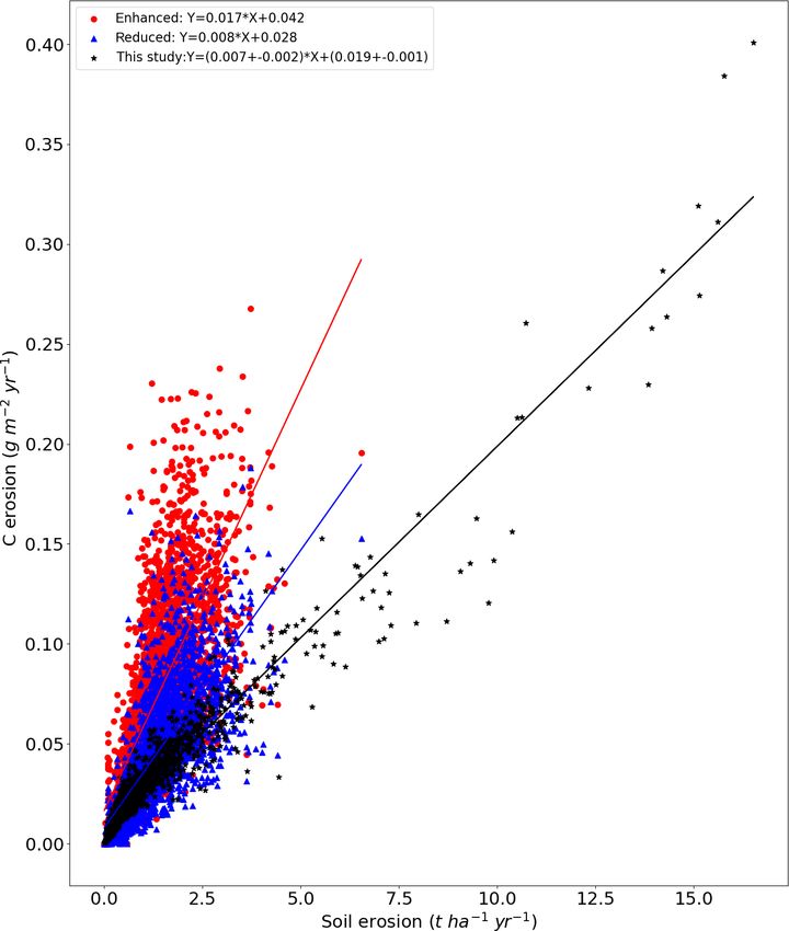
V. Naipal et al.: CE-DYNAM (v1)                                                                                                1205

af and bf are constants that relate f to the average topo-
graphical slope (θ) of a grid cell depending on the type of
land cover. θmax is the maximum topographical slope of the
entire Rhine catchment.
   The parameters af and bf are chosen in such a way that
f varies between 0.2 and 0.5 for cropland, reflecting the de-
creased sediment connectivity between hillslopes and flood-
plains created by artificial structures such as ditches and
hedges. For natural vegetation such as forests and natural
grassland, af and bf are chosen in a way that f varies be-
tween 0.5 and 0.8, assuming that in these landscapes hill-
slopes and floodplains are well connected. This assumption
on the reduced sediment connectivity for agricultural land-
scapes is supported by several previous studies on the effect
of erosion on sediment yield (Hoffmann et al., 2013a; De
Moor and Verstraeten, 2008; Gumiere et al., 2011; Wang et
al., 2015). These studies showed that anthropogenic activi-
ties on agricultural landscapes result in a trapping of eroded
soil in colluvial deposition sites, reducing the sediment trans-
port from hillslopes to floodplains. The model parameter f
has been calibrated for the Rhine catchment by Naipal et
al. (2016), where the ranges mentioned above are found to
produce a ratio between hillslope and floodplain sediment
                                                                   Figure 2. The Rhine catchment (Hoffmann et al., 2013a), where the
storage that was comparable to observations. The studies by
                                                                   gray shades represent elevation and the continuous black lines the
Wang et al. (2010, 2015) identified a range for the hillslope      main rivers.
sediment delivery to be between 50 % and 80 %, which is
similar to the range in the (1 − f ) factor in our model. In
each case and within the defined boundaries, the slope gra-        to be calibrated based on local data of sediment ages before
dient determines the final value of f . Eroded material that       CE-DYNAM can be applied to other catchments.
has not been deposited in the floodplains is assumed to be            Floodplain SOC storage follows the same residence time
deposited at the foot of the hillslopes as colluvial sediment.     as sediment on top of the actual decomposition rate of C in a
   The floodplain fractions of the grid cells are connected        grid cell of ORCHIDEE. The routing of sediment and C be-
through a 5 arcmin resolution flow-routing network (Naipal         tween the grid cells follows a multiple-flow routing scheme.
et al., 2016), where the rivers and streams are indirectly in-     In this scheme the flow coming from a certain grid cell is dis-
cluded in the floodplain area but not explicitly simulated. By     tributed across all lower-lying neighbors based on a weight
routing the sediment and C through the floodplain fractions        (W , dimensionless) that is calculated as a function of the con-
of grid cells, we lump together the slow process of riverbank      tour length (c):
erosion by river dynamics (timescale is approximately equal
                                                                                         θ(i+k,j +l) × c(i+k,j +l)
to a few years to thousands of years), and the rather fast pro-    W(i+k,j +l) =                                        .        (7)
                                                                                     k,l=1
cess of transport of eroded material by the rivers (timescale                         P
                                                                                            θ(i+k,j +l) × c(i+k,j +l)
is approximately equal to days). The rate by which sediment                         k,l=−1
and SOC leave the floodplain of a grid cell to go to the flood-
plain of an adjacent grid cell is determined by the sediment       Here, c is 0.5 × grid size (m) in the cardinal direction and
residence time. The sediment residence time (τ ) is a function     0.354 × grid size (m) in the diagonal direction. (i, j ) is the
of the upstream contributing area (Flowacc):                       grid cell in consideration where i counts grid cells in the lati-
                                                                   tude direction and j in the longitude direction. i +k and j +l
            Flowacc(i)−aτ
τ (i) = e        bτ         .                               (6)    specify the neighboring grid cell where k and l can be either
                                                                   −1 0 or 1; θ is calculated as the division between the differ-
The study by Hoffmann et al. (2008) showed that the major-         ence in elevation (h) given in meters and the grid cell size
ity of floodplain sediments have a residence time that ranges      (d) (also in meters):
between 0 and 2000 years, with a median of 50 years. The                           h(i,j ) − h(i+k,j +l)
constants aτ and bτ are chosen in such a way that basin τ          θ(i+k,j +l) =                         .                       (8)
                                                                                             d
varies between the 5th and 95th percentiles of those obser-
vations, with a median for the whole catchment of 50 years.        The sediment and C routing is done continuously at a daily
These constants are uniform for the whole basin, and need          time step to preserve the numerical stability of the model. A

www.geosci-model-dev.net/13/1201/2020/                                                  Geosci. Model Dev., 13, 1201–1222, 2020
1206 V. Naipal et al.: CE-DYNAM (v1)
more detailed explanation of the methods presented in this from a dataset on 120 000 yield observations over the 20th
section can be found in the study by Naipal et al. (2016). century in northeast French departments (NUTS3 adminis-
trative division) (Schauberger et al., 2018). According to the
2.4 Litter dynamics yield data assembled by Schauberger et al. (2018), yields in
northeast France (covering part of the Rhine catchment) for
The four litter pools in the emulator are an belowground and these crops increased fourfold during the last century. Note
an aboveground litter pool, each split into a metabolic and that crop residues like straw constituted a larger fraction of
structural pool with different turnover rates as implemented the total biomass in 1850 than in 2005, but those residues
in ORCHIDEE (Krinner et al., 2005). The belowground lit- were likely collected and used for animal feed and housing
ter pools consist mostly of root residues. Both the biomass fuel. We did not account for this harvest of residue in the
and litter pools have a loss flux due to fire as incorporated simulation of SOC.
into ORCHIDEE by the SPITFIRE model of Thonicke et
al. (2010). The litter that is not respired or burned is trans- 2.6 SOC dynamics without erosion
ferred to the SOC pools based on the CENTURY model (Par-
ton et al., 1987), which was modified by Naipal et al. (2018) The change in the C content of the PFT-specific SOC pools
to include a vertical discretization scheme for SOC. in the emulator without soil erosion was described by Naipal
The vertical discretization scheme was introduced in the et al. (2018) (Fig. 1) as follows:
emulator to account for a declining C input and SOC respi-
ration with depth, and it consists of 20 soil layers with 10 cm dSOCa (t)
= lita (t) + kpa × SOCp (t) + ksa
thickness each. The litter-to-soil fluxes from aboveground lit- dt
ter pools are all attributed to the top 10 cm of the soil profile. × SOCs (t) − kap + kas + k0a × SOCa (t) ,
The litter-to-soil fluxes from belowground litter pools are dis- (10)
tributed exponentially over the whole soil profile according
to
Ibe (z) = I0be × e−r×z . (9) dSOCs (t)
= lits (t) + kas × SOCa (t)
dt
Here, I0be is the belowground litter input to the surface soil − ksa + ksp + k0s × SOCa (t) , (11)
layer and r is the PFT-specific vertical root-density attenua-
tion coefficient as used in ORCHIDEE. The sum of all layer-
dependent litter-to-soil fractions is equal to the total litter to dSOCp (t)
soil flux as calculated by ORCHIDEE. The vertical SOC pro- = kap × SOCa (t) + ksp × SOCs (t)
dt
file is modified by erosion and the resulting deposition rates,
− (kpa + k0p ) × SOCp (t) . (12)
which is discussed in detail in the following sections.
Here, SOCa , SOCs , and SOCp (g C m−2 ) are the active, slow,
2.5 Crop harvest and yield and passive SOC, respectively. The distinction of these SOC
pools, defined by their residence times, are based on the study
We adjusted the representation of crop harvest from OR-
by Parton et al. (1987). The active SOC pool has the lowest
CHIDEE by assuming a variable harvest index for C3 plants
residence time (1–5 years) and the passive the highest (200–
that increases during the historical period as shown in the
1500 years). lita and lits (g C m−2 d−1 ) are the daily litter in-
study of Hay (1995) for wheat and barley, which are also
put rates to the active and slow SOC pools, respectively; k0a ,
the main C3 crops in the Rhine catchment. The harvest index
k0s , and k0p (d−1 ) are the respiration rates of the active, slow,
is defined by the ratio of harvested grain biomass to above-
and passive pools, respectively; kas , kap , kpa , ksa , and ksp are
ground dry matter production (Krinner et al., 2005). In this
the coefficients determining the flux from the active to the
study the harvest index increases linearly between 0.26 and
slow pool, from the active to the passive pool, from the pas-
0.46 (Naipal et al., 2018), which is consistent with the aver-
sive to the active pool, from the slow to the active pool, and
age values of Hay (1995).
from the slow to the passive pool, respectively.
Furthermore, we found that in certain cases the cropland
The vertical C discretization scheme in the emulator as-
net primary productivity (NPP) was too high during the en-
sumes that the SOC respiration rates decrease exponentially
tire period of 1850–2005, especially in the early part of the
with depth:
20th century. This is because the cropland photosynthetic
rates were adjusted in ORCHIDEE to give a cropland NPP ki (z) = k0i (z) × e−re×z . (13)
representative of present-day values that are higher than for
the low input agriculture of the early 20th century. To de- Here, ki is the respiration rate at a soil depth z, and “re”
rive a more realistic NPP for wheat and barley in the Rhine (m−1 ) is a coefficient representing the impact of external fac-
catchment, we used the long-term crop yield data obtained tors, such as decreasing oxygen availability with depth. k0 is
Geosci. Model Dev., 13, 1201–1222, 2020 www.geosci-model-dev.net/13/1201/2020/V. Naipal et al.: CE-DYNAM (v1) 1207
the respiration rate of the surface soil layer for a certain SOC Hillslope erosion without the deposition term has already
pool i. The variable re is determined in such a way that the been tested and applied at the global scale as part of the C
total soil respiration of a certain pool over the entire soil pro- removal model presented by Naipal et al. (2018).
file without erosion is similar to the output of the full OR-
CHIDEE model. A detailed description of how this is done
can be found in the study by Naipal et al. (2018).
2.8 C deposition and transport in floodplains
2.7 Net C erosion on hillslopes
In the model we assume that soil erosion takes place on hill-
slopes and not in the floodplains, due to the usually low topo- The SOC-profile dynamics of floodplains are controlled by
graphical slope of floodplains. The factor (1 − f ) determines (1) C input from the hillslopes, (2) C import by lateral trans-
the fraction of the eroded soil that is deposited in the collu- port from the floodplain fractions of upstream grid cells, and
vial reservoirs (Fig. 1, Eq. 4b). Soil erosion always removes (3) C export to the floodplain fractions of downstream grid
a fraction of the SOC stock in the upper soil layer depend- cells (Fig. 1). First, the net erosion flux from the surface layer
ing on the erosion rate and bulk density of the soil. The next of the hillslope fraction of the grid cell (kE ×SOCHS at z = 0)
soil layer contains less C and therefore at the following time is incorporated into the surface layer of the floodplain. At
step less C will be eroded under the same erosion rate. In the the same deposition rate, the SOC of the surface layer of the
model, the SOC-profile evolution is dynamically tracked and floodplain is incorporated into the subsoil layer. Similarly, a
updated at a daily time step, which conforms with the method fraction of the SOC of the subsoil layer is moved downward
of Wang et al. (2015). First, a fraction of the C from each soil one layer. We will refer to this process as the “downward”
pool in proportion to the erosion rate is removed from the moving of C in the soil layer profile. It should be noted that
surface layer. Then, at the same erosion rate, SOC from the C selectivity during transport and deposition is not taken into
subsoil layer becomes the surface layer, maintaining the soil account here, meaning that the C pools of the deposited ma-
layer thickness in the vertical discretization scheme. Simi- terial are the same as the eroded material from the topsoil
larly, the SOC from the subsoil later also moves upward one of eroding areas. At the same time as deposition takes place
layer. The removal of C by erosion triggers a compensatory a fraction of the C of the surface layer proportional to the
C sink due to the reduction in SOC respiration on eroding sediment residence time (τ ) is exported out of the catchment
land. This compensatory C sink and reduced C erosion over following the sediment routing scheme, resulting in the “up-
time will ultimately lead to an equilibrium state. The change ward” moving of the C from the subsoil layers. This process
in C content due to net erosion (the eroded sediment or C represents the river bank erosion and resulting POC export
that leaves the hillslopes after deposition) of the PFT-specific by the water network, although rivers and streams are not
pools for hillslopes can be represented by the following equa- explicitly represented in the model. As we do not have infor-
tions: mation on the subgrid spatial distribution of land cover frac-
tions, we first sum the exported C flux over all PFTs before
dSOCHSi (z, t) assigning the flux proportionally to the land cover fractions
= kE × SOCHSi (z + 1, t) − kE
dt of the receiving downstream-located grid cells. The C that is
× SOCHSi (z, t) , (14) imported from the neighboring grid cells follows the same
procedure as the deposition of eroded material, and this re-
where dSOCHSi (z, t) is the change in hillslope SOC of a sults in a downward moving of the C in the soil profile. The
component pool i at a depth z and at time step t. The daily change in C content due to deposition and routing of the PFT-
net erosion fraction, kE (dimensionless), is calculated as the specific SOC pools for floodplains can be represented by the
following: following equations:
E
f × 365
kE = × EF, (15)
BD × dz
where E is the gross soil erosion rate (t ha−2 yr−1 ) (note “ha” dSOCFLi (z, t)
represents hectare), f is the floodplain deposition factor, BD = kD + kiout × SOCFLi (z − 1, t)
dt
is the average bulk density of the soil profile (g cm−3 ), dz
1
is the soil thickness (equal to 0.1 m), and EF is the C en- + × SOCFLi (z + 1, t)
(τ × 365)
richment factor that is set to 1 by default. A model sensitiv-
ity analysis will be performed (see Sect. 4.3) with EF > 1 to 1
− kD + + kiout
represent a higher C concentration in eroded soil compared (τ × 365)
to the original soil as a result of the selectivity of erosion. × SOCFLi (z, t)) , for z > 0; (16)
www.geosci-model-dev.net/13/1201/2020/ Geosci. Model Dev., 13, 1201–1222, 20201208 V. Naipal et al.: CE-DYNAM (v1)
cell as reconstructed by Peng et al. (2017) (Table 1). Peng et
al. (2017) derived historical changes in PFT fractions based
dSOCFLi (0, t) Xn=9
= kiout (n) × SOCFLi (0, t) (n) on the LUHv2 land use dataset (Hurtt et al., 2011), histori-
dt n=1
cal forest area data from Houghton (2003), and the present-
+ (kE × SOCHSi (0, t)) day forest area from ESA CCI satellite land cover (Euro-
1 pean Space Agency, 2014). By using different transition rules
+ × SOCFLi (1, t) and independent forest data to constrain the changes in crop
(τ × 365)
1
and urban PFTs, they derived the most suitable historical
− kD + + kiout PFT maps.
(τ × 365)
When land use change takes place, the litter and SOC
× SOCFLi (0, t)) , for z = 0; (17) pools of all shrinking PFTs are summed and allocated pro-
portionally to the expanding PFTs, maintaining the mass bal-
where n is the neighboring grid cell that flows into the current
ance. In this way the litter pools and SOC stocks get im-
grid cell, dSOCFLi (z, t) is the change in floodplain SOC of a
pacted by different input and respiration rates for each soil
component pool i at a depth z and at time step t, and SOCHS
layer. When forest is reduced, three wood products with de-
is the hillslope SOC stock. kD is the deposition rate and equal
cay rates of 1, 10, and 100 years are formed and harvested.
to
The biomass pools of other shrinking land cover types are
kE × AREAHS transformed to litter and allocated to the expanding PFTs.
kD = , (18)
AREAFL More details on the land use scheme are described in the
study by Naipal et al. (2018).
where AREAHS is the hillslope area and AREAFL is the
floodplain area (m2 ) of a grid cell. kiout is the import rate 2.10 Study area
per C pool i from neighboring grid cells (dimensionless) and
can be calculated as The model is tested for the Rhine catchment (Fig. 2), which
n=9 has a total basin area of about 185 000 km2 covering five dif-
P 1
(W × τ ×365 × AREAFL ) (n) ferent countries in central Europe. Its large size is benefi-
n=1 cial for the application of a coarse-resolution model such as
kiout = , (19)
AREAFL CE-DYNAM to study large-scale regional dynamics in the
where W is the weight index of Eq. (7). C cycle due to soil erosion. The Rhine catchment has a con-
The first term of Eq. (16) represents the downward mov- trasting topography, with steep slopes larger than 20 % up-
ing of the incoming C related to the C deposition flux from stream in the Alps, and large, wide, and flat floodplains at the
the hillslope fraction of the grid cell and the lateral C import foot of the Alps, the Upper Rhine, and the Lower Rhine. The
flux from the floodplain fractions of upstream neighboring floodplains store large amounts of sediment and C that orig-
grid cells. The second term represents the upward moving of inate from eroding hillslopes upstream. These sediment stor-
SOC related to the lateral C transfer to downstream neigh- ages provide the possibility to study the long-term effect of
boring grid cells. The third term of Eq. (16) represents the erosion on hillslope and floodplain dynamics. Furthermore,
total C loss flux from the current soil layer z, which is a re- the Rhine catchment has been experiencing different stages
sult of either the upward or downward moving of the C in the of land use change over the Holocene, with land degrada-
soil profile. The first term of Eq. (17) represents the incoming tion dating back to more than 5500 years ago (Dotterweich,
lateral C flux from the floodplains of the upstream neighbor- 2013). In contrast, during the last 2 decades there has been
ing grid cells. The second term represents the C deposition a general afforestation and soil erosion has been decreasing.
flux coming from the hillslope fraction of the grid cell. The These land use changes and changes in erosion make an in-
third term represents the upward moving of the SOC from teresting and important case to study the effect of anthro-
the subsoil layer to the topsoil layer as a result of sediment pogenic activities on the C cycle in Europe.
or C routing. The last term of Eq. (17) represents the total In addition, the Rhine catchment has been the focus of
loss of C from the topsoil layer, of which part is distributed many erosion studies providing observations on erosion and
across the neighboring grid cells downstream ( (τ ×365)1
), and sediment dynamics that can be used for model validation
part is moved “downwards” in the soil profile as a result of (Asselman, 1999; Asselman et al., 2003; Erkens, 2009; Hoff-
C deposition (kD ) and the incoming lateral C from upstream mann et al., 2007, 2008, 2013a, b; Naipal et al., 2016). The
grid cells (kiout ). global sediment budget model that forms the basis for the
sediment dynamics scheme of CE-DYNAM has been val-
2.9 The land use change bookkeeping model idated and calibrated for the Rhine catchment with obser-
vations on sediment storage from Hoffmann et al. (2013a)
The land use change bookkeeping scheme includes the yearly and scaling relationships between sediment storage and basin
changes in forest, grassland, and cropland areas in each grid area (Naipal et al., 2016). Hoffmann et al. (2008, 2013a) did
Geosci. Model Dev., 13, 1201–1222, 2020 www.geosci-model-dev.net/13/1201/2020/V. Naipal et al.: CE-DYNAM (v1) 1209
an inventory of 41 hillslope and 36 floodplain sediment and Table 2. Model simulations, with changes to the basin average gross
SOC deposits related to soil erosion over the last 7500 years. soil erosion rate (t ha−1 yr−1 ), the basin average sediment residence
The floodplain sediment observations consist mostly of or- time τ (years), the enrichment factor, and the crop residue harvest
ganic material (gyttja, peat) and fine sediments (fine sand, intensity RM (%).
loam, silt) in overbank deposits (Hoffmann et al., 2008).
These fine sediments are a result of long-term soil erosion Default Gross soil Enrichment
on the hillslopes. Hoffmann et al. (2013a) found that the simulations erosion τ factor RM
sediment and SOC deposits were quantitatively related to S0 0 – – 0
the basin size according to certain scaling functions, where S1 3.94 94 1 0
floodplain deposits increased in a nonlinear way with basin S2 3.94 94 1 0
size, while the hillslope deposits showed a linear increase Uncertainty
with basin size. We use these relationships to validate the simulations
spatial variability in SOC storage of floodplains and hill-
slopes simulated by CE-DYNAM. The scaling relationships S1_min 1.52 94 1 0
S2_min 1.52 94 1 0
have the form of a simple power law:
S1_max 5.95 94 1 0
A b S2_max 5.95 94 1 0
M =a× , (20)
Aref Sensitivity
simulations
where M is the sediment storage or the SOC storage, a is the
storage (Mt) related to an arbitrary chosen area Aref , and b is S2_Tmin 3.94 60 1 0
the scaling exponent. S2_Tmax 4.94 128 1 0
S1_EF 5.94 94 2 0
2.11 Input data and model simulations S2_EF 6.94 94 2 0
S0_RM 0 – – 100
To create the C emulator that forms the underlying C cycle S1_RM 3.94 94 1 100
of CE-DYNAM, we first ran the full ORCHIDEE model for S2_RM 3.94 94 1 100
the period 1850–2005 at a coarse resolution of 2.5◦ latitude
and 3.75◦ longitude, and we output all C pools and fluxes.
The pools and fluxes were then archived together and used daily time step. After each year the subbasins exchanged the
to derive the turnover rates to build the emulator. The SOC lateral C fluxes with each other.
scheme of the emulator that has been modified to account for We also performed seven additional sensitivity simula-
soil erosion processes was made to run at a spatial resolu- tions and four additional uncertainty simulations. Simulation
tion of 5 arcmin, similar to the original global sediment bud- S1_EF and S2_EF are performed to test the model assump-
get model. Then, we performed three main simulations with tion of C enrichment during erosion. Here, we changed the
CE-DYNAM for the Rhine catchment. Simulation S0 is the enrichment factor EF to 2, based on the study by Lugato
baseline simulation or no-erosion simulation, where SOC dy- et al. (2018). Simulations S2_Tmin and S2_Tmax are per-
namics are similar to the full ORCHIDEE model. Simulation formed to test the rate of C transport between floodplains.
S1 is the erosion-only simulation, where the hillslopes erode Here we modified the mean sediment residence time for the
and all eroded C is respired to the atmosphere without reach- Rhine catchment to a minimum of 60 years (50 % lower than
ing the colluvial and alluvial deposition sites. Simulation S2 the current value) and to a maximum of 128 years (50 %
is the simulation with full sediment dynamics, where hill- higher than the current value), respectively. However, we
slopes and floodplains are connected and can store or lose C. kept the maximum sediment residence time at 1500 years.
We ran the emulator for 3000 years at a daily time step with Simulations S0_RM, S1_RM, and S2_RM are performed
the initial climate and land cover of the period 1850–1860. To to test the model assumption on crop residue management,
speed up the spin-up simulations we calculated the temporary where we assumed that all aboveground crop litter is har-
equilibrium state of the floodplain SOC pools every 10 years vested.
analytically. At the end of the spin-up period the floodplain For the uncertainty analysis, we performed simulations
SOC pools were close to equilibrium, with a yearly change S1_min and S2_min based on a minimum soil erosion sce-
of less than 0.001 % of the total floodplain SOC stock. After- nario and S1_max and S2_max based on a maximum soil
wards, we performed the transient simulations for the period erosion scenario. These soil erosion scenarios are derived
1851–2005 at a daily time step with changing climate and from the uncertainty ranges in the rainfall erosivity and land
land cover conditions, using the equilibrium SOC stocks as cover factors of the erosion model. All the model simulations
baseline. To ensure a faster performance of CE-DYNAM, we are summarized in Table 2.
delineated the Rhine catchment into seven large subbasins
and ran the model in parallel for each of the subbasins at a
www.geosci-model-dev.net/13/1201/2020/ Geosci. Model Dev., 13, 1201–1222, 20201210 V. Naipal et al.: CE-DYNAM (v1)
2.12 Validation methods and data sively employed to estimate net fluxes of sediments across
hillslopes at catchment and regional scales.
For the validation of C erosion rates, we used the high-
We performed a detailed model validation of the sediment resolution model results from Lugato et al. (2018), where
and the C parts of the model according to the following steps: they coupled the RUSLE2015 erosion model to the CEN-
(1) validation of soil erosion rates using observational and TURY biogeochemistry model. These model results were
high-resolution model estimates for Germany and Europe, available at a resolution of 1 km, where each grid cell was
(2) validation of C erosion rates using high-resolution model composed of an erosion and deposition fraction. The C ero-
estimates for Europe from Lugato et al. (2018), (3) validation sion rates provided by Lugato et al. (2018) were multiplied
of the spatial variability of hillslope and floodplain C storage with the erosion fraction of a 1 km grid cell. Then, the C ero-
using observational results from Hoffmann et al. (2013a), sion rates were aggregated to the resolution of CE-DYNAM.
and (4) validation of SOC stocks using observational data Lugato et al. (2018) provided an enhanced and a reduced
from a global soil database and a European land use survey. erosion-induced C sink uncertainty scenario, based on dif-
The validation of the soil erosion module has been done ferent assumptions for C enrichment, burial, and C mineral-
before in the studies by Naipal et al. (2015, 2016). However, ization during transport. In CE-DYNAM the C erosion rates
we do it again in this study due to different input datasets. In from simulation S1 are multiplied with the hillslope area to
addition, the validation includes soil erosion data from new get the total C erosion flux of a grid cell. As the study by Lu-
global soil erosion studies such as Borrelli et al. (2018) and gato et al. (2018) considers only agricultural areas, we con-
Panagos et al. (2015). For the validation of gross soil ero- sidered only the crop fraction of a grid cell during the com-
sion rates, we used the high-resolution model estimates of parison. It should be noted that the SOC dynamics scheme
Panagos et al. (2015), who applied the RUSLE2015 model of CE-DYNAM, which is derived from ORCHIDEE LSM,
at a 100 m resolution at European scale for the year 2010. is also based on the CENTURY model. However, there are
Similarly to the Adj.RUSLE, RUSLE2015 is also derived large differences between the CENTURY model used by Lu-
from the original RUSLE model. However, in contrast to gato et al. (2018) and the C dynamics scheme of ORCHIDEE
our model, RUSLE2015 does include the erosion factors L used in this study. For example, in the CENTURY model
and P . Furthermore, our model uses more coarsely resolved the crop productivity is mediated by nitrogen availability,
input datasets (Table 1), for which the equations for the R which is not the case in the ORCHIDEE version used for
and S factors have been modified. Thus, even though both this study. The CENTURY model also includes some man-
Adj.RUSLE and RUSLE2015 are derived from the same ero- agement practices such as crop rotations, which are not rep-
sion model, the differences between the models are large, resented in ORCHIDEE. The CENTURY model runs at a
which justifies our model comparison. The extensive vali- much higher resolution and is calibrated for agricultural land,
dation of the Adj.RUSLE model in this study and previous while ORCHIDEE also simulates forest, grasslands, and bare
studies (Naipal et al., 2015, 2016, 2018) shows that despite soil. In this way, the final SOC stocks derived with CE-
its coarse resolution, it is applicable at large spatial scales. DYNAM are also a result of erosion from other land cover
Furthermore, we used independent high-resolution erosion types and land use changes. This is an important feature for
estimates from the study by Cerdan et al. (2010), available at land use change, which is not included in the CENTURY
a 1 km resolution at European scale, which were based on model. Furthermore, the ORCHIDEE LSM has been used in
an extensive database of measured erosion rates under natu- many global intercomparisons and extensively evaluated for
ral rainfall in Europe. For the comparison, we aggregated the C budgets (Müller et al., 2019; Todd-Brown et al., 2013). Fi-
high-resolution model results of both datasets to the resolu- nally, ORCHIDEE also includes the last century change in
tion of CE-DYNAM. We also used the potential soil erosion crop production calibrated against data (Guenet et al., 2018).
map of the Federal Institute for Geosciences and Natural Re- For the validation of the spatial variability of the SOC
sources of Germany (Bug et al., 2014) for comparison. This stocks of hillslopes and floodplains, we used the scaling re-
map presents the yearly-average soil erosion rates at a 250 m lationships between basin area and SOC storage derived by
resolution on agricultural land derived from a USLE-based Hoffmann et al. (2013a). The study by Naipal et al. (2016)
approach (Universal Soil Loss Equation), with some modi- found that the global sediment budget model is able to repro-
fications to the erosion factors and input data. Before vali- duce the scaling behavior of sediment storage. After analyz-
dating our model results we aggregated these high-resolution ing the dependence of this scaling behavior, they argue that
erosion rates also to the coarser resolution of our model. it is an emergent feature of the model and mainly dependent
Validation of our net soil erosion rates is done based on on the underlying topography. This indicates that the scaling
the 100 m resolution net soil erosion rates derived with features of floodplain and hillslope sediment and C storage
the WATEM/SEDEM model (Borrelli et al., 2018). WA- should also be applicable to a more recent time period. In or-
TEM/SEDEM simulates soil removal by water erosion based der to evaluate the ability of CE-DYNAM to reproduce this
on the USLE approach, sediment transport, and deposition scaling behavior for SOC, we selected the grid cells that con-
based on the transport capacity. The model has been exten- tained the points of observation of the study by Hoffmann et
Geosci. Model Dev., 13, 1201–1222, 2020 www.geosci-model-dev.net/13/1201/2020/V. Naipal et al.: CE-DYNAM (v1) 1211
al. (2013a) and performed a regression of the basin area (de-
fined as the upstream contributing area) and the SOC storage
for floodplains and hillslopes separately. Comparing the ab-
solute values of the sediment and SOC storages of each grid
cell from Hoffmann et al. (2013a) was not possible due to the
difference in the time period of the studies, where Hoffmann
et al. (2013a) focused on the entire Holocene, while our study
focused only on the period starting from 1850 CE.
For the validation of the total SOC stocks, we used the
Global Soil Dataset for Earth system modeling (GSDE)
(Shangguan et al., 2014), available at a spatial resolution
of 1 km, and the Land Use/Land Cover Area Frame Survey
(LUCAS) (Palmieri et al., 2011). The LUCAS topsoil SOC
stocks, available at a high spatial resolution of 500 m, were
calculated using the LUCAS SOC content for Europe (de
Brogniez et al., 2015) and soil bulk density derived from soil
texture datasets (Ballabio et al., 2016).
3 Results
Figure 3. Quantile box-and-whisker plots of simulated gross soil
Due to large uncertainties in the model and validation data erosion rates (t yr−1 ) (gray box-and-whisker plots) compared to
for the Alpine region, we only present and discuss the model (a) the study by Cerdan et al. (2010), (b) the study by Panagos
and validation results for the non-Alpine part of the Rhine et al. (2015), and (c) the German potential erosion map by Bug et
catchment. al. (2014) (orange box-and-whisker plots). (d) Quantile box-and-
whisker plots of simulated net soil erosion rates (t yr−1 ) (gray box-
3.1 Model validation and-whisker plots) compared to the study by Borrelli et al. (2018)
(orange box-and-whisker plots). Medians are plotted as red horizon-
In this section we present the model validation results using tal lines. The x axis represents bins or evenly spaced ranges between
the minimum and maximum total yearly soil erosion rates of the
the methods and data described in detail in the previous sec-
Rhine derived from the data of (a) Cerdan et al. (2010), (b) Panagos
tion.
et al. (2015), (c) Bug et al. (2014), and (d) Borrelli et al. (2018).
We find that the quantile distribution of the simulated gross
soil erosion rates compares well to the distributions of other
observational and high-resolution modeling studies (Cerdan
et al., 2010; Panagos et al., 2015; Bug et al., 2014), al- net soil erosion, our model results are different to those of
though CE-DYNAM usually underestimates the very large the study by Borrelli et al. (2018) due to the different ap-
soil erosion rates such as is found by Cerdan et al. (2010) proaches in calculating the sediment deposition. For exam-
(Fig. 3a, b, c). This is due to the coarse spatial and temporal ple, in our study the deposition of sediment in hillslopes is
resolution of CE-DYNAM, and the lack of the slope-length explicitly calculated as a function of the slope and vegetation
factor (L). (Cerdan et al., 2010, assumed a constant slope type or cover. Borrelli et al. (2018) used the transport capac-
length of 100 m.) It should be noted that our study, Cerdan ity concept (Van Rompaey et al., 2001). Both methods have
et al. (2010), and Bug et al. (2014) simulated potential soil their uncertainties when applied at large spatial scales. The
erosion rates that were not accounting for EC practices rep- method in our study has been designed and calibrated to be
resented by the P factor. used at a large spatial scale and at coarse resolution, while
We also find that the quantile distribution of the simulated the method of Borrelli et al. (2018) was originally designed
net soil erosion from hillslopes compares well with the distri- to be applied at spatial scales < 100 m.
bution from the high-resolution modeling study by Borrelli et We find that the quantile distributions of our simulated
al. (2018) (Fig. 3d). In addition we performed a spatial com- agricultural C erosion and deposition rates are similar to
parison of our simulated gross and net erosion rates to those those of the high-resolution modeling study by Lugato et
of the studies mentioned above. For this purpose, we delin- al. (2018) (Fig. 4a–d). Also the spatial variability of the C
eated 13 subbasins in the Rhine catchment (Fig. S3 in the erosion rates at subbasin level is in good comparison to the
Supplement). Table 3 summarizes the resulting goodness- validation data (Table 4). However, the linear regression be-
of-fit statistics of this comparison and shows that for gross tween soil erosion and C erosion rates of our study lies at the
soil erosion our erosion model is generally in good agree- lower end of the relationships derived from the enhanced and
ment with the other studies at subbasin level. However, for reduced erosion scenarios of Lugato et al. (2018) (Fig. 5).
www.geosci-model-dev.net/13/1201/2020/ Geosci. Model Dev., 13, 1201–1222, 20201212 V. Naipal et al.: CE-DYNAM (v1)
Table 3. Goodness-of-fit results of the comparison of the simulated
gross and net erosion rates to those of other studies at subbasin level,
taking into account 13 subbasins of the Rhine. RMSE is the root
mean square error in 106 t yr−1 . E stands for soil erosion.
E Cerdan E E E Borrelli
et al. (2010) Germany RUSLE2015 et al. (2018)
r squared 0.72 0.97 0.94 0.24
RMSE 0.68 1.98 0.92 1.35
Table 4. Goodness-of-fit results of the comparison of the simulated
gross and net C erosion rates to those of the study by Lugato et
al. (2018) in the enhanced and reduced scenario, taking into account
13 subbasins of the Rhine. RMSE is the root mean square error in
t yr−1 . Ce stands for gross C erosion, while Cd stands for net C
erosion.
Ce Ce Cd Cd
enhanced reduced enhanced reduced
r squared 0.95 0.95 0.98 0.98
RMSE 7977 13 797 3450 9822 Figure 4. (a) Hillslope C erosion rates and (b) C deposition
rates compared to the enhanced erosion scenario from Lugato et
al. (2018). (c) Hillslope C erosion rates and (d) C deposition rates
compared to the reduced erosion scenario from Lugato et al. (2018).
On the one hand, our study does not include EC practices,
The x axis represents bins or evenly spaced ranges between the min-
leading to substantially larger simulated soil erosion rates in
imum and maximum total yearly soil erosion rates of the Rhine.
regions with EC. Figure 5 shows that our simulated erosion
rates are in general larger than the erosion rates from Lugato
et al. (2018), which may be explained by this mechanism. tween the simulated floodplain SOC storage and basin area
On the other hand, the C erosion rates of our study are lower compared to the simulated hillslope SOC storage when us-
than those of Lugato et al. (2018), due to the coarse spatial ing the grid cells that contain the points of observation corre-
resolution of our underlying C scheme derived from the OR- sponding to the study by Hoffmann et al. (2013a). This result
CHIDEE LSM. The decreased spread in our simulated values is in line with what Hoffmann et al. (2013a) found, and it
is also a result of the coarse resolution of our model. shows that CE-DYNAM can realistically reproduce the spa-
Accounting for erosion, deposition, and transport of SOC tial variability in SOC stocks between hillslopes and flood-
leads to a better representation of the simulated topsoil C plains (Table 6). However, when deriving the scaling rela-
stocks per land cover type when compared to SOC stocks of tionships at subbasin level instead of using individual grid
the LUCAS database (Fig. 6). The simulated SOC stocks of cells, we do not find a significant difference in the scaling
the top 20 cm of the soil profile fall within the quantile range between floodplains and hillslopes (Table 6).
of the LUCAS SOC stocks for cropland and forest (Fig. 6).
Although the topsoil SOC stocks for grassland improved, a 3.2 Model application
large uncertainty range remains. Furthermore, we find that in
both the erosion and no-erosion simulations the SOC stocks We find an average annual soil erosion rate of 1.44 ±
for grassland are higher than for forest. This is also observed 0.82 t ha−1 yr−1 over the period 1850–2005, which is about
in the study by Wiesmeier et al. (2012), where they found half of the average erosion rate simulated for the last mil-
considerably higher SOC stocks for grassland with a median lennium (Naipal et al., 2016) and falls within the range of
of 11.8 kg C m−2 compared to forest based on the analysis the average erosion rates of the Holocene (Hoffmann et al.,
of 1460 soil profiles in southern Germany. Furthermore, the 2013a). This soil erosion flux mobilized around 66 ± 28 Tg
comparison of the simulated total SOC stocks to those of the of C over the same time period, of which on average 57 % is
LUCAS and GSDE databases at subbasin level shows a good deposited in colluvial reservoirs, 43 % is deposited in alluvial
model performance with respect to the spatial variability in reservoirs, and 0.2 % is exported out of the catchment.
topsoil SOC stocks (Table 5). The lower average annual soil erosion rate over the study
To validate the spatial variability of floodplain and hill- period compared to the last millennium is a result of the gen-
slope SOC stocks separately, we used the scaling relation- eral afforestation in the non-Alpine part of the Rhine catch-
ships found by Hoffmann et al. (2013a) (Sect. 2.12). We find ment that started around 1910 CE according to the data on
a significantly larger exponent for the scaling relationship be- land cover and land use (Peng et al., 2017; Fig. 7b). This land
Geosci. Model Dev., 13, 1201–1222, 2020 www.geosci-model-dev.net/13/1201/2020/You can also read