Inter-comparison of snow depth over Arctic sea ice from reanalysis reconstructions and satellite retrieval
←
→
Page content transcription
If your browser does not render page correctly, please read the page content below
The Cryosphere, 15, 345–367, 2021
https://doi.org/10.5194/tc-15-345-2021
© Author(s) 2021. This work is distributed under
the Creative Commons Attribution 4.0 License.

Inter-comparison of snow depth over Arctic sea ice from reanalysis
reconstructions and satellite retrieval
Lu Zhou1 , Julienne Stroeve2,3,4 , Shiming Xu1,5 , Alek Petty6,7 , Rachel Tilling6,7 , Mai Winstrup8,9 , Philip Rostosky10 ,
Isobel R. Lawrence11 , Glen E. Liston12 , Andy Ridout2 , Michel Tsamados2 , and Vishnu Nandan3
1 Ministry  of Education Key Laboratory for Earth System Modeling, Department of Earth System Science,
Tsinghua University, Beijing, China
2 Centre for Polar Observation and Modelling, Earth Sciences, University College London, London, UK
3 Centre for Earth Observation Science, University of Manitoba, Winnipeg, Canada
4 National Snow and Ice Data Center, University of Colorado, Boulder, CO, USA
5 University Corporation for Polar Research, Beijing, China
6 NASA Goddard Space Flight Center, Greenbelt, MD, USA
7 Earth System Science Interdisciplinary Center, University of Maryland, College Park, MD, USA
8 DTU Space, Technical University of Denmark, Lyngby, Denmark
9 Danish Meteorological Institute (DMI), Copenhagen, Denmark
10 Institute of Environmental Physics, University of Bremen, Bremen, Germany
11 Centre for Polar Observation and Modelling, University of Leeds, Leeds, UK
12 Colorado State University, Cooperative Institute for Research in the Atmosphere (CIRA), Fort Collins, CO, USA

Correspondence: Julienne Stroeve (stroeve@nsidc.org)

Received: 25 February 2020 – Discussion started: 9 March 2020
Revised: 21 November 2020 – Accepted: 25 November 2020 – Published: 27 January 2021

Abstract. In this study, we compare eight recently developed      depths retrieved from Operational IceBridge (OIB) while
snow depth products over Arctic sea ice, which use satel-         correlations are quite low against buoy measurements, with
lite observations, modeling, or a combination of satellite and    no correlation and very low variability from University of
modeling approaches. These products are further compared          Bremen and DMI products. Inconsistencies in reconstructed
against various ground-truth observations, including those        snow depth among the products, as well as differences be-
from ice mass balance observations and airborne measure-          tween these products and in situ and airborne observations,
ments. Large mean snow depth discrepancies are observed           can be partially attributed to differences in effective footprint
over the Atlantic and Canadian Arctic sectors. The differ-        and spatial–temporal coverage, as well as insufficient obser-
ences between climatology and the snow products early in          vations for validation/bias adjustments. Our results highlight
winter could be in part a result of the delaying in Arctic        the need for more targeted Arctic surveys over different spa-
ice formation that reduces early snow accumulation, lead-         tial and temporal scales to allow for a more systematic com-
ing to shallower snowpacks at the start of the freeze-up sea-     parison and fusion of airborne, in situ and remote sensing
son. These differences persist through spring despite over-       observations.
all more winter snow accumulation in the reanalysis-based
products than in the climatologies. Among the products eval-
uated, the University of Washington (UW) snow depth prod-
uct produces the deepest spring (March–April) snowpacks,          1   Introduction
while the snow product from the Danish Meteorological In-
stitute (DMI) provides the shallowest spring snow depths.         Snow on sea ice plays an important role in the Arctic cli-
Most snow products show significant correlation with snow         mate system. Snow provides freshwater for melt pond devel-
                                                                  opment and, when the melt ponds drain, freshwater to the

Published by Copernicus Publications on behalf of the European Geosciences Union.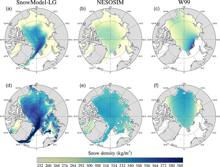
346                                                         L. Zhou et al.: Inter-comparison of snow depth over Arctic sea ice

upper ocean (Eicken et al., 2004). In winter, snow insulates        evaluate them against various in situ observations and differ-
the underlying sea ice cover, reducing heat flux from the ice–      ent NASA Operation IceBridge (OIB) snow depth products.
ocean interface to the atmosphere and slowing winter sea            Since these data sets do not have common spatiotemporal
ice growth (Sturm and Massom, 2017). Snow also strongly             resolutions, we limit our comparisons to monthly averages
reflects incoming solar radiation, impacting the surface en-        between October–November (from now referred to as the au-
ergy balance and under-ice algae and phytoplankton growth           tumn period) and March–April (spring period) from 2000 to
(Mundy et al., 2009). Furthermore, sea ice thickness cannot         2018 and also limit our region to the Arctic basin (i.e., we ex-
be retrieved from either laser or radar satellite altimetry with-   clude regions such as the Sea of Okhotsk, Bering Sea, Baffin
out good knowledge of both the snow depth and snow density          Bay and Davis Strait, and the East Greenland Sea).
(Giles et al., 2008; Kwok, 2010; Zygmuntowska et al., 2014).           The paper is organized as follows. The next section de-
   Despite its recognized importance, snow depth and density        scribes the details of each snow product, snow depth ob-
over the Arctic Ocean remain poorly known. Most of our un-          servations and climatology data used for comparison. Com-
derstanding comes from measurements collected from Soviet           parisons among snow products and between climatologies
North Pole drifting stations and limited field campaigns. The       are shown in Sect. 3. Section 4 discusses validation against
Warren et al. (1999) climatology and the recently updated           OIB and buoy measurements and representation issues. The
Shalina and Sandven (2018) climatology, hereafter W 99 and          conclusion and further implications for snow are found in
SS18, respectively, have provided a basic understanding of          Sect. 5.
the seasonally and spatially varying snow depth distribution
over Arctic sea ice. However, these data were collected from
stations between 1950 and 1991 and were largely confined            2     Data and methods
to multiyear ice (MYI) in the central Arctic. Hence, they are
                                                                    In this section, we introduce (1) observational data sets of
not representative of the Arctic-wide snow cover characteris-
                                                                    snow depth used for validation/comparison, (2) climatolog-
tics of recent years (Webster et al., 2014). Today, the Arctic
                                                                    ical snow depth products, (3) passive and active microwave
Ocean has transitioned from a regime dominated by thicker,
                                                                    snow depth products, and (4) reconstructed snow depth es-
older MYI to one dominated by thinner and younger first-
                                                                    timates from models. The inter-comparison among all snow
year ice (FYI) (Maslanik et al., 2007, 2011). In addition, the
                                                                    products and comparison between these products and mea-
length of the ice-free season has increased (delayed freeze-up
                                                                    surements are based on their native spatial and temporal res-
and early melt onset/breakup), reducing the amount of time
                                                                    olution. However, the spatial and temporal resolution varies
over which snow can accumulate on the sea ice (Stroeve and
                                                                    considerably between products. Details on resolution and
Notz, 2018). In response to this data gap, several groups are
                                                                    grids are provided in Table 1.
working to produce updated assessments of snow on sea ice
                                                                       An additional comparison was made between OIB and
using a variety of techniques.
                                                                    the different snow depth products at the coarsest spatial
   From satellites, several studies have used passive mi-
                                                                    (100 × 100 km) grid and temporal (monthly) resolution. Be-
crowave brightness temperatures to retrieve snow depth, on
                                                                    low we briefly describe each data set. We refer the reader to
FYI (Markus et al., 2011) and MYI (Rostosky et al., 2018;
                                                                    the references for each data product for more detailed infor-
Kilic et al., 2019; Braakmann-Folgmann and Donlon, 2019;
                                                                    mation on the individual algorithms.
Winstrup et al., 2019). Other studies have modeled snow ac-
cumulation over sea ice using various atmospheric reanaly-          2.1     Measurements used for comparison
sis products as input (Blanchard-Wrigglesworth et al., 2018;
Petty et al., 2018; Liston et al., 2020; Tilling et al., 2020).     2.1.1    In situ observations
Some promise has also been shown in mapping snow depth
by combining satellite-derived radar freeboards from two            Ice mass balance buoys (IMBs) are designed to provide snow
different radar altimeters (Lawrence et al., 2018; Guerreiro        depth and ice thickness information and have generally been
et al., 2016) and from active–passive microwave satellite syn-      deployed within undeformed MYI (Richter-Menge et al.,
ergies (Xu et al., 2020). With the launch of ICESat-2, addi-        2006). In this study, we use snow depth measurements from
tional possibilities exist to combine radar and lidar altimeters    IMBs deployed by US Army Cold Regions Research and En-
to directly retrieve snow depth (Kwok and Markus, 2018).            gineering Laboratory (CRREL). Each buoy is equipped with
Such approaches are paving the way for proposed future              acoustic sounders above and below the ice with an accuracy
satellite missions (i.e., ESA’s CRISTAL, Kern et al., 2019).        5 mm for depth measurements (Richter-Menge et al., 2006).
   In recognition of the numerous new snow data products            Following Perovich et al. (2021), snow depth measurements
available, it is timely to provide an inter-comparison of these     greater than 2 m or less than 0 m are removed. In total, 58
products so that recommendations can be made to the sci-            CRREL buoy tracks are used between 2010 and 2015 (avail-
ence community as to which data product best suits their            able at: http://imb-crrel-dartmouth.org, last access: 13 Jan-
needs. Towards this end, we provide a comprehensive in-             uary 2021). To align the IMB data with the daily and monthly
tercomparison between eight new snow depth products and             snow depth products, as well eliminate effects from missing

The Cryosphere, 15, 345–367, 2021                                                        https://doi.org/10.5194/tc-15-345-2021
L. Zhou et al.: Inter-comparison of snow depth over Arctic sea ice                                                                                   347

Table 1. Summary of investigated snow reconstruction products.

   Product         Time span    Temporal resolution   Spatial grids    Projection type            Method type               Reference
   SnowModel-LG    1980–2018    All year (daily)      25 × 25 km       EASE grid                  Reanalysis-based          Liston et al. (2020),
                                                                                                                            Stroeve et al. (2020)
   NESOSIM         2000–2017    August to April       100 × 100 km     Polar stereographic grid   Reanalysis-based          Petty et al. (2018)
                                (daily)
   CPOM            1991–2017    All year (daily)      10 × 10 km       Polar stereographic grid   Reanalysis-based          Tilling et al. (2020)
   UW              1980–2015    April                 75 × 75 km       Polar stereographic grid   Reanalysis-based          Blanchard-Wrigglesworth
                                (monthly)                                                                                   et al. (2018)
   DuST            2003–2008,   Every 2 months        1.5◦ long        Up to 81.5◦ N              Active satellite-based    Lawrence et al. (2018)
                   2013–2018    (2013–2018)           × 0.5◦ lat
                                and monthly
                                (2003–2008)
   DESS            2011–2019    March                 12.5 × 12.5 km   Polar stereographic grid   Active and passive        Xu et al. (2020)
                                (monthly)                              (up to 87.5◦ N)            satellite-based
   PMW Bremen      2003–2018    March and April       25 × 25 km       Polar stereographic grid   Passive satellite-based   Rostosky et al. (2018)
                                (daily)
   PMW DMI         2013–2018    January to April      25 × 25 km       EASE grid 2.0              Passive satellite-based   Winstrup et al. (2019)
                                (daily)

measurements, we average the IMB data into monthly av-                     ferent algorithms show general agreement in regional snow
erages after first creating daily averages from the 4-hourly               depth distributions, larger interannual variability is observed
observations. See Table S1 in the Supplement for a listing of              among these algorithms than found in W 99, and mean snow
buoys used, along with their dates/time periods of operation.              depth differences result from different ways of detecting
   Snow buoys have been deployed by the Alfred Wegener                     the snow–air and snow–ice interfaces from the radar returns
Institute (AWI) since 2010 (Nicolaus et al., 2017) and pro-                (Kwok et al., 2017). Taking these differences into consider-
vide snow depth estimates from four separate snow depth                    ation, we use four OIB snow depth products from the (1)
pingers. These are averaged together to provide one snow                   Sea Ice Freeboard, Snow Depth, and Thickness data quick-
depth value at each buoy location. Here, we use snow depths                look product (quicklook) available from NSIDC website and
from 28 AWI snow buoys between 2013–2017 (accessible at:                   examined in King et al. (2015) and Kwok et al. (2017); (2)
http://data.meereisportal.de, last access: 13 January 2021),               NASA Goddard Space Flight Center (GSFC) (Kurtz et al.,
which are also listed in Table S1. Similar to the CREEL                    2013, 2015); (3) Jet Propulsion Laboratory (JPL) (Kwok and
buoys, the snow depths are first averaged into daily averages              Maksym, 2014); and (4) snow radar layer detection (SRLD)
before monthly averages are derived.                                       (Koenig et al., 2016). These four OIB products overlap only
                                                                           in 2014 and 2015, and thus we limit our comparisons with
2.1.2   OIB airborne observations                                          OIB-derived snow depths to those 2 years. Each OIB product
                                                                           is first regridded to the 100×100 km polar stereographic pro-
Since 2009, NASA Operation IceBridge (OIB) has con-                        jection, and then all daily flight tracks are averaged together
ducted airborne profiling of Arctic sea ice every spring, gen-             to produce monthly mean OIB snow depths (March or April)
erally across the western Arctic. Snow depth observations are              for each year. We also compare snow reconstructions on their
derived with an ultra-wideband quicklook snow radar (Paden                 native spatiotemporal resolution with OIB measurements in
et al., 2014), capable of retrieving snow depth from the radar             the Supplement.
echoes from both air–snow and snow–ice interfaces (Kurtz
and Farrell, 2011). Snow depth can then be retrieved through               2.2     Snow depth climatologies
retracking and compensation from the radar echogram. The
OIB campaigns provide unique large-scale and high-spatial-                 In addition to the airborne and in situ snow measurements,
resolution observations; however, the swath is limited due to              we use two types of conventional large-scale snow prod-
the airborne nature of the measurements. Furthermore, most                 ucts that are often used in the derivation of sea ice thick-
flight tracks cover a limited area from the north of Greenland             ness from radar or laser altimetry (Ricker et al., 2014; Kwok
towards Alaska, and data cover only a limited time period,                 and Cunningham, 2008), the Warren et al. (1999) (W 99) and
namely March and April.                                                    the Shalina and Sandven (2018) (SS18) climatologies. W 99
   Several algorithms have been developed to derive snow                   provides distributions of snow depth and density for each cal-
depth from this radar system (Kwok et al., 2017). While dif-               endar month by assembling North Pole (NP) drifting station

https://doi.org/10.5194/tc-15-345-2021                                                                   The Cryosphere, 15, 345–367, 2021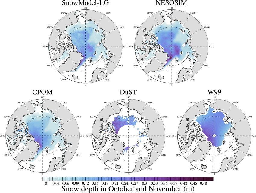
348                                                        L. Zhou et al.: Inter-comparison of snow depth over Arctic sea ice

observations from the 1950s to 1990s. A two-dimensional            models (Xu et al., 2020). Each approach uses vastly differ-
quadratic function is adopted to fit the measurements to the       ent methodologies and provides snow information at differ-
Arctic basin. W 99 also provides a climatology of snow wa-         ent spatial and temporal resolutions.
ter equivalent (SWE) from January to December. This is de-
rived using snow depths and densities measured along snow          2.3.1   Reanalysis-based snow depth reconstruction
lines, and, if unavailable, Arctic-mean density for that month
is used. Like snow depth, a two-dimensional quadratic fit was      SnowModel-LG
applied to the SWE data.
   SS18 further combines NP data (as in W 99) with addi-           SnowModel-LG is a prognostic snow model originally devel-
tional snow data from the Soviet airborne expeditions (Sever)      oped for terrestrial snow applications, now adapted for snow
obtained primarily during the 1960s to 1980s to produce            depth reconstruction over sea ice using Lagrangian ice par-
spring (March–April–May) snow depth fields. Since the air-         cel tracking (Liston et al., 2020). Physical snow processes
craft would land on level FYI, SS18 is not limited to MYI in       are included such as blowing snow redistribution and sub-
the central Arctic (as W 99) but includes FYI in the Eurasian      limation, density evolution, and snowpack metamorphosis.
seas as well (Shalina and Sandven, 2018). The spatial grid         SnowModel-LG is used in a Lagrangian framework to redis-
spacing of the SS18 climatology is 100 × 100 km within the         tribute snow around the Arctic basin as the sea ice moves.
Arctic basin.                                                      Tracking begins on 1 August 1980, assuming snow-free ini-
                                                                   tial conditions, and accumulates snow until 31 July of the
2.3   Satellite- and model-based snow depth products               next year. On 31 July, any remaining snow that is isother-
                                                                   mal and saturated with meltwater becomes superimposed
Eight snow depth data sets are included in this inter-             ice and is no longer identified as “snow”. SnowModel-LG
comparison study (Table 1). They mainly fall into two cat-         is the only data product that includes snow depth during
egories: (1) snow reconstruction using atmospheric reanal-         the melt season. The essential inputs to this data product
ysis data as input to a snow accumulation model together           are atmospheric reanalysis estimates of precipitation, 2 m
with snow redistribution by sea ice drift; (2) snow depth          air temperature, wind speed and direction, and weekly ice
retrieved from satellite data, including passive-microwave-        motion vectors from NSIDC (Stroeve et al., 2020). Weekly
based snow retrieval, blended satellite-derived radar sea ice      ice motion vectors are linearly interpolated to daily resolu-
freeboards at two different frequencies, and active–passive        tion. Outputs relevant to this study are the snow depth and
satellite (combining CryoSat-2 and SMOS) data synergy.             bulk snow density (Liston et al., 2020) and are provided
Here, snow depth is defined as the average thickness of snow       on a 25 × 25 km EASE grid. A recent study (Stroeve et al.,
over the entire grid-cell area for eight products, not just over   2020) evaluated SnowModel-LG using NASA MERRA-2
the sea-ice-covered fraction.                                      (Gelaro et al., 2017) and ERA5 atmospheric reanalysis fields
   The first category includes four different new products: the    (Hersbach and Dee, 2016) against several data sets includ-
distributed snow evolution model (SnowModel-LG) (Liston            ing OIB, IMBs, MagnaProbe and passive microwave esti-
et al., 2020; Stroeve et al., 2020), NASA Eulerian Snow on         mates. They found that the model captured observed spatial
Sea Ice Model (NESOSIM) (Petty et al., 2018), the Centre           and seasonal variability in snow depth accumulation, while
for Polar Observation and Modelling (CPOM) model (Till-            also showing statistically significant declines in snow depth
ing et al., 2020), and the Lagrangian Ice Tracking System          since 1980 during the cold season. The temporal resolution
for snowfall over sea ice from the University of Washing-          of SnowModel-LG is daily between 1 August 1980 and 31
ton (UW) (Blanchard-Wrigglesworth et al., 2018). The sec-          July 2018.
ond category includes the following snow depth products:
the products from the University of Bremen (PMW Bremen)            NESOSIM
(Rostosky et al., 2018) and the Danish Meteorological In-
stitute (PMW DMI) (Winstrup et al., 2019) rely on satellite        The NASA Eulerian Snow On Sea Ice Model (NESOSIM)
passive microwaves at multiple frequencies and polarizations       is a three-dimensional, two-layer (vertical), Eulerian snow
for their snow depth retrieval algorithms. The Dual-altimeter      budget model (Petty et al., 2018). NESOSIM includes two
Snow Thickness (DuST) product (Lawrence et al., 2018) is           snow layers: old compacted snow and new fresh snow. Wind-
derived from combining data from CryoSat-2 (Ku band) and           packing and snow loss to the leads are included and were
AltiKa (Ka band) satellite radar altimeters. The DuST prod-        used to calibrate NESOSIM with historical snow depth and
uct also combines Envisat (radar altimeter: Ku band) and           density observations from the NP drifting station data. NE-
ICESat (laser altimeter) data during their period of overlap.      SOSIM was run using several atmospheric reanalyses, in-
Finally, Department of Earth System Science in Tsinghua            cluding ERA-Interim (ERA-I) (Dee et al., 2011), JRA-55
University (DESS) combines a Ku-band altimeter (CryoSat-           (Ebita et al., 2011) and MERRA (Rienecker et al., 2011), and
2) and L-band passive microwave radiometer (SMOS) to re-           a median of these daily reanalysis snowfall estimates is used
trieve snow depth and sea ice thickness based on two physical      in this study. The model is also forced with near-surface wind

The Cryosphere, 15, 345–367, 2021                                                      https://doi.org/10.5194/tc-15-345-2021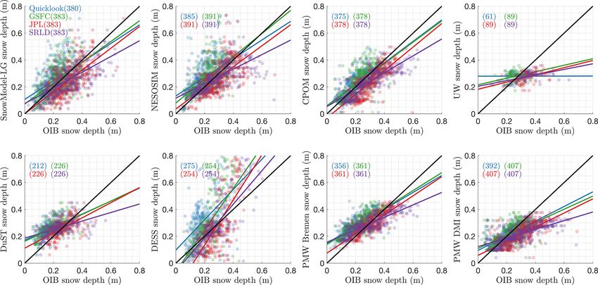
L. Zhou et al.: Inter-comparison of snow depth over Arctic sea ice                                                            349

fields from ERA-I, NSIDC Polar Pathfinder sea ice drift vec-      UW
tors (Tschudi et al., 2019) and Bootstrap passive microwave
ice concentrations (Comiso, 2017). Snow accumulation is           The last reanalysis-based snow reconstruction is from the
initialized at the end of summer (default of 15 August) and       University of Washington (UW). The algorithm accumulates
run until the following spring (1 May). To initialize snow        cold-season snowfall along sea ice drift trajectories using 12-
depth in mid-August, NESOSIM linearly scales the August           hourly snowfall from ERA-I, weekly NSIDC sea ice vec-
snow depth in the W 99 climatology based on the ratio be-         tors and weekly-averaged NOAA-NSIDC sea ice concentra-
tween duration of the summer melt season and the climato-         tion (Meier et al., 2013). A Lagrangian Ice Tracking System
logical summer duration. The duration of the summer melt          (LITS) (DeRepentigny et al., 2016) is used to backward track
season is defined based on ERA-I air temperatures, and cli-       each grid point from the first week of April to the last week of
matological summer melt duration is from Radionov et al.          the previous August (Blanchard-Wrigglesworth et al., 2018).
(1997). Snow depth is further equally divided into the “old”      This tracking system has a claimed accuracy of ≈ 50 km af-
and “new” snow layers, with snow transferred from the new         ter 6 months of tracking (DeRepentigny et al., 2016). Once
to the old snow layer based on the wind conditions. Snow          the 6-month trajectories are established for each ice parcel,
is then accumulated and evolves dynamically with sea ice          the algorithm accumulates weekly-averaged snowfall along
motion through a divergence–convergence and an advection          each parcel trajectory. A sea ice concentration correction is
term. Daily snow depth (mean depth over the sea ice frac-         further imposed every week (one time step). Specifically, if
tion) and snow density and snow volume (per unit grid cell)       the ice concentration drops below 15 %, the accumulation
are available from 15 August to 30 April for each year, at a      stops and the trajectory is ended at the previous time step.
spatial grid spacing of 100 × 100 km in a polar stereographic     Only monthly snow depths in April are available for the pe-
projection. NESOSIM provides the effective snow depth of          riod from 1980 to 2015. Spatial grid spacing of the data set
the ice-covered fraction and the mean grid-cell snow depth.       is 75 × 75 km on a polar stereographic projection.
In order to be consistent with snow depth estimates from the
other methods, we will use the latter in this study.              2.3.2   Satellite-based snow depth retrieval

                                                                  DuST
CPOM
                                                                  Lawrence et al. (2018) derives snow depth by utilizing the
                                                                  difference in freeboards retrieved from radar altimeter satel-
The CPOM snow depth product (Tilling et al., 2020) is ini-        lites operating at different frequencies. Specifically, satel-
tialized on a Lagrangian grid with a spacing of 10 km run-        lite data from ESA’s CryoSat-2 (CS-2, Ku-band radar satel-
ning from 40◦ N to the pole. Snow accumulation begins on          lite altimeter operational since 2010) and CNES/ISRO’s Al-
15 August each year using the W 99 August snow depth and          tiKa (Ka-band radar satellite altimeter, 2013–present) are
a fixed density of 350 kg m−3 on all ice-covered (sea ice con-    used. The deviation of each satellite’s return from its ex-
centration > 15 %) grid points. This initial snow layer is kept   pected dominant scattering horizon (the snow surface for
separated from any accumulated snow after the model has           the Ka band and the ice–snow interface for the Ku band) is
started running. The model then steps daily through the win-      quantified using independent snow and ice freeboards from
ter, accumulating snow in SWE. Snow parcels are moved us-         OIB. Using a spatially variable correction function, AltiKa
ing NSIDC Polar Pathfinder ice motion data, and any parcels       and CS-2 freeboards are calibrated to the snow surface and
moving outside the ice-covered region are removed. New            snow–ice interfaces, respectively, allowing snow depth to be
parcels covered by expansion of the ice-covered region be-        estimated as the difference between the two. A caveat to the
come active with no initial snow. Where the 2 m ERA-I air         approach is that since OIB data are only available during
temperature is above freezing point, the daily ERA-I SWE          March and April and cover limited regions of the Arctic, the
of snowfall is added to the already accumulated column.           calibration of the CS-2 and AltiKa freeboards with OIB may
A fraction of the accumulated snow is removed when the            not be valid during other months and/or regions. The same
wind speed exceeds 5 m s−1 using a function proportional to       methodology has also been applied to ICESat and Envisat
wind speed and lead fraction (see Schröder et al., 2019, Ta-      satellites, whose active periods overlap between 2003 and
ble 1). Finally, the total column of accumulated SWE at each      2009, and these data are used to extend the snow depth prod-
Lagrangian point is converted to snow depth using a daily         uct further back in time. This Dual-altimeter Snow Thick-
snow density function constructed in a similar way to Kwok        ness (DuST) product produces (1) monthly snow depth maps
and Cunningham (2008), which is added to the initial snow         from October to April during the CS-2/AltiKa period (2013–
layer (if present). The irregularly spaced snow data from the     present) and (2) bimonthly (every 2 months) annual snow
Lagrangian grid are re-gridded onto a regular 10 km2 polar        depth maps (March–April or October–November) during the
stereographic projection using an averaging radius of 50 km       ICESat–Envisat period (2003–2008). For both time periods,
to give a snow depth map for each day of winter.                  the snow depth is gridded on a 1.5◦ longitude × 0.5◦ latitude

https://doi.org/10.5194/tc-15-345-2021                                                    The Cryosphere, 15, 345–367, 2021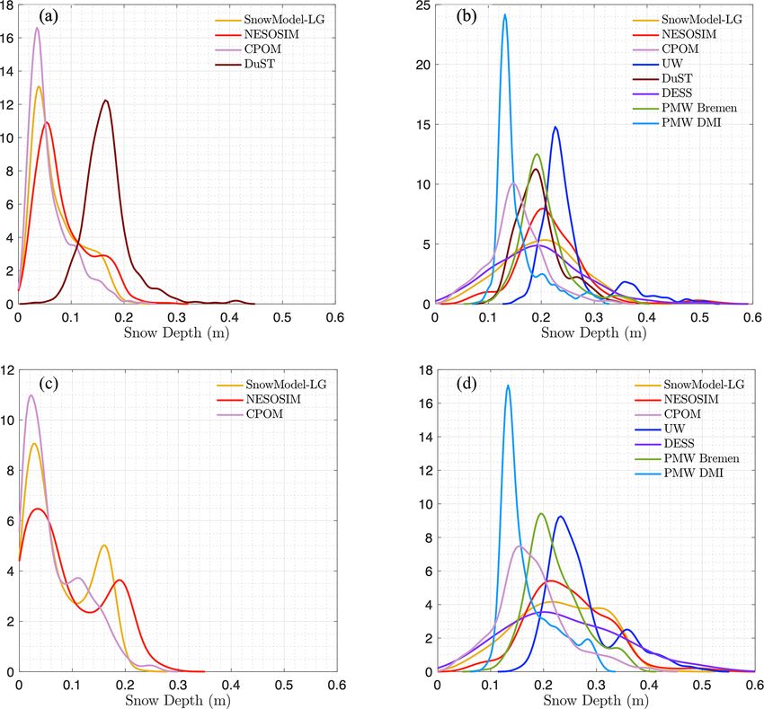
350                                                     L. Zhou et al.: Inter-comparison of snow depth over Arctic sea ice

grid. The data are limited to below 81.5◦ N due to the upper    PMW DMI
latitude of AltiKa/Envisat.
                                                                In Winstrup et al. (2019), snow depth is derived by a ran-
                                                                dom forest regression model based on passive microwave
                                                                Tbs from AMSR-E and AMSR2. The model was trained us-
PMW Bremen                                                      ing a Round-Robin Data Package (Pedersen et al., 2018),
                                                                with OIB campaigns snow thicknesses provided by NSIDC
                                                                including IDCSI4 and quicklook products and collocated
The University of Bremen’s PMW snow depth product de-           brightness temperatures. Training was performed on two-
scribed in Rostosky et al. (2018) on FYI is available dur-      thirds of the data set, using OIB data from the period April
ing the AMSR-E/2 period. The algorithm is adapted from          2009–March 2014, leaving the remaining OIB data (period:
Markus and Cavalieri (1998), which was derived from a           March 2014–April 2015) for validation purposes. Specifi-
series of passive microwave sensors, such as the Scan-          cally, multi-channel Tbs ranging from the C band (6.9 GHz)
ning Multichannel Microwave Radiometer (SMMR) (from             to 89 GHz are included as predictors, at both vertical and
1979), and continuing on through the Special Sensor Mi-         horizontal polarization. The random forest consists of 500
crowave/Imager (SSM/I) and SSM/I Sounder (SSMIS). The           regression trees, each derived from bootstrapping the input
latter algorithm computes the spectral gradient ratio between   data and using a maximum limit of five predictors for each
18.7 and 37 GHz vertical polarization brightness tempera-       leaf in the regression trees. The most important predictors,
tures (Tbs) to generate 5 d averaged snow depth estimations     as found by the algorithm, were the following channels:
over FYI (Markus et al., 2011). This algorithm has limita-      18.7 GHz (27 %), 23.8 GHz (17 %) and 10.7 GHz (11 %), all
tions for wet snow spring and multiyear ice (Comiso et al.,     vertical polarizations. Derived snow depths were found to be
2003) and large sensitivity to surface roughness (Stroeve       in good agreement with the OIB data retained for validation,
et al., 2006). Snow depths over smooth FYI were found to        with an average error of 0.05 m and an accuracy of 78.7 %.
be accurate in comparisons with OIB during 2009 and 2011        The passive microwave snow depth product from the Dan-
(RMSE < 0.06 m over a shallow snow cover), while signif-        ish Meteorological Institute (PMW DMI) constructs spring-
icant biases were found over rougher FYI or MYI (Brucker        time (March and April) daily snow depth between 2013 and
and Markus, 2013).                                              2018 at 25 × 25 km spatial grid spacing on the EASE-Grid
   Rostosky et al. (2018) further extends the approach of       2.0 (Brodzik et al., 2012).
Markus and Cavalieri (1998) to also include snow depth over
MYI using the lower frequencies of 6.9 GHz from the NASA        DESS
Advanced Microwave Scanning Radiometer for the Earth
Observing System (AMSR-E) and the JAXA Global Change            The Department of Earth System Science in Tsinghua Uni-
Observation Mission – Water (GCOM-W) AMSR2 instru-              versity (DESS) algorithm retrieves both sea ice thickness and
ment. We refer to the resulting product as the PMW Bre-         snow depth simultaneously by using sea ice freeboard from
men snow depth product. The gradient ratio between verti-       CS2 and the L band (1.4 GHz) Tbs from the Soil Moisture
cal polarized brightness temperatures (Tbs) at 18.7 GHz and     and Ocean Salinity (SMOS) satellite (Xu et al., 2020). The
6.9 GHz helps to mitigate the retrieval sensitivity problems    active periods of these two satellites are both from 2010 to
over MYI during March and April. Specifically, robust linear    present. Specifically, this algorithm combines a hydrostatic
regressions were derived based on fitting 5 year (2009, 2010,   equilibrium model and improved L-band radiation model
2011, 2014, and 2015) of the NOAA Wavelet (WAV) Air-            (Xu et al., 2017). Sea ice freeboard is converted to sea ice
borne Snow Radar-Snow Depth on Arctic Sea Ice Data Set          thickness based on hydrostatic equilibrium (Laxon et al.,
(Newman et al., 2014) and the polarized Tb gradient ratio.      2003), using assumptions on snow, ice and water densities.
Snow depths over different ice types were fitted separately,    Tbs from SMOS can be used to retrieve thin sea ice thick-
using the Ocean and Sea Ice Satellite Application Facility      ness (Kaleschke et al., 2012) and snow depth over thick ice
(OSI-SAF) sea ice type map to distinguish between FYI and       (Maaß et al., 2013(@). The L-band radiation model is fur-
MYI. No evaluation/validation was performed in regions out-     ther improved by adding vertical structure of temperature
side of OIB measurements. The spatial grid spacing is similar   and salinity in sea ice and snow (Zhou et al., 2017). In or-
to typical passive microwave measurements, at 25×25 km in       der to obtain the missing measurements resulting from lim-
the polar stereographic projection. Daily snow depth maps       ited upper latitude in the SMOS satellite, L-band Tbs span-
for winter months from November to April since 2002 are         ning inclination angles from 0 to 40◦ and from 85 to 87.5◦ N
available. It should be noted that snow depth over MYI is       are approximated using Tbs of all frequencies in AMSR-E
only available during March and April when the OIB data         and AMSR2 through a back-propagation machine-learning
were available to constrain the model. Snow depth uncer-        process. By combining the two observational data sets, the
tainty is estimated to be between 0.1 and 6.0 cm over FYI       uncertainties in both sea ice thickness and snow depth are
and between 3.4 and 9.4 cm over MYI.                            largely reduced. Unlike optimal interpolation-based sea ice

The Cryosphere, 15, 345–367, 2021                                                   https://doi.org/10.5194/tc-15-345-2021
L. Zhou et al.: Inter-comparison of snow depth over Arctic sea ice                                                                  351

thickness synergy, as applied in Ricker et al. (2017), the un-
certainty in ice thickness is reduced through an explicitly re-
trieved snow depth.
   Both sea ice thickness and snow depth are available in the
DESS product. Here we use the monthly snow depth maps
available for March of each year since 2011, which are pro-
vided at a spatial grid spacing of 12.5 × 12.5 km on a polar
stereographic projection.

3     Snow products inter-comparison                                Figure 1. The common regions (yellow) of snow product inter-
                                                                    comparison with (a) and without (b) DuST. Also shown are the re-
In this section, we carry out a systematic comparison of            gions of interest in this study: Canadian Arctic (CA), North Atlantic
the eight snow products, using the two climatological snow          sector (Atlantic), and Pacific and Central Arctic (Pacific).
data sets (W 99 and SS18) as a reference for all comparisons
and analyses. Section 3.1 presents the results for mean snow
depth and its spatial distribution, Sect. 3.2 introduces the sea-   land Sea (NESOSIM in particular) and the Atlantic sector of
sonal cycle, and the long-term trend and interannual variabil-      the Arctic. Despite some general agreements, mean spring
ity is presented in Sect. 3.3. For the two products that model      snowpack and regional discrepancies are evident in Fig. 2.
an evolving snow density, we also intercompare these against        In particular, the thickest snow in late winter/early spring for
climatology (Sect. 3.4). While we focus on basin-wide es-           NESOSIM occurs in the East Greenland Sea, while in DESS
timates for the whole Arctic, we also explore consistency           the deepest snow is concentrated in the Canadian Arctic.
and mean state of all products over three sub-regions: the             During autumn, for the region north of Greenland and
Canadian Arctic sector (CA) including the Canadian Arc-             Svalbard, SnowModel-LG runs forced with MERRA-2 show
tic Archipelago, the Atlantic (Atlantic), and the Pacific and       a similar spatial pattern to other reanalysis-based modeling
Central Arctic (Pacific) sectors (regions outlined in Fig. S1).     systems (i.e., NESOSIM and CPOM) but shallower snow
Over these regions, sea ice conditions vary considerably, with      than NESOSIM (Fig. 3). DuST also shows deep snowpacks
mostly thick MYI within the CA and thinner FYI elsewhere.           in this region (16.6 cm mean snow depth), though the spatial
The North Atlantic has generally more precipitation as a re-        coverage is more limited. Spring snow depth, ranging from
sult of proximity to the North Atlantic storm tracks.               15.2 to 25.3 cm in the Arctic domain (Fig. 1), exhibits large
   Given the relatively long time period and basin-scale cov-       spatial variability among all products. Further, relatively
erage provided by SnowModel-LG, this snow depth prod-               thick snowpacks in the North Atlantic sector are evident
uct is used as the reference product when carrying out the          in all reanalysis-based products except for CPOM. Deeper
regional consistency checks. To align the temporal and spa-         snowpacks are expected in this region as it receives win-
tial resolution between all snow products, comparisons are          ter precipitation from the North Atlantic storm tracks. The
mainly carried out after year 2000 and focused on the early         discrepancies in spring among the reanalysis-based products
and late winter months of October and/or November and               are the results of several aspects including initial snow as-
March and/or April. The products containing data for longer         sumption, tracking numerical algorithm and reanalysis adop-
time periods are further explored against climatologies, and        tion. For comparison, snow is also the deepest (over 35 cm)
their long-term trends are assessed.                                to the north of Svalbard in both the W 99 and SS18 clima-
                                                                    tologies. NESOSIM further suggests thick snow over Davis
3.1    Mean state and distribution of snow depth                    Strait, with spring averaged snow depths greater than 25 cm.
                                                                    This is in stark contrast to the other data sets over the FYI
Mean snow depth, which is a direct indicator of total snow          in that region and is likely unrealistic given this is a region
volume over sea ice, is of fundamental importance for the           of first-year ice that does not usually freeze until December
characterization of the Arctic hydrological cycle. Spatial          and/or January, e.g., Stroeve et al. (2014), limiting the time
maps of monthly mean snow depth across all data products,           over which snow can accumulate on the ice.
as well as the W 99 and SS18 climatologies, are shown in               The histogram of time-averaged snow depth in the differ-
Figs. 2 and 3 in spring (autumn) months for the season of           ent products is shown in Fig. 4 for the period 2000 to 2018
2014–2015. Products are shown with their native resolution          during the spring and autumn periods, respectively. Out of
and grids. The spatial patterns in all products are in broad        all the reanalysis-based data products, snow depth distribu-
agreement that thicker snow occurs north of Greenland and           tions in NESOSIM are shifted towards slightly deeper snow-
the CA sector and thinner snow in the seasonal ice zones            packs (8.4 cm) than those from SnowModel-LG (7.2 cm) and
(i.e., Baffin Bay and marginal seas of the Eurasia continent).      CPOM (6.0 cm) during autumn, although the shapes of the
Some products also show thicker snow in the East Green-             distributions are similar. The deepest snowpacks during Oc-

https://doi.org/10.5194/tc-15-345-2021                                                        The Cryosphere, 15, 345–367, 2021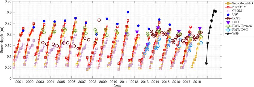
352                                                        L. Zhou et al.: Inter-comparison of snow depth over Arctic sea ice

Figure 2. Mean snow depth (units: m) in spring (March–April) 2014 for eight snow products, W 99 and SS18.

Figure 3. Mean snow depth (units: m) in autumn (October–November) 2014 for four snow products and W 99.

The Cryosphere, 15, 345–367, 2021                                                         https://doi.org/10.5194/tc-15-345-2021
L. Zhou et al.: Inter-comparison of snow depth over Arctic sea ice                                                              353

tober and/or November are found in DuST, with a mode of            snow depth on perennial and seasonal ice. It is worth not-
the distribution at about 16.6 cm. This is much larger than        ing that this agreement is across the two distinctive meth-
other products and seems unlikely to be realistic early in the     ods for snow depth reconstruction, i.e., the reanalysis-based
snow accumulation season. During spring (Fig. 4b), PMW             numerical integration and satellite-based retrievals. This is
DMI exhibits the overall smallest snow depth in late winter        also reflected in both the basin-scale snow depth averages
(14.5 cm), while UW shows the largest snow depth (25.2 cm)         and the spatial patterns. However, the areas where the thick-
in the common region of the snow products. Conclusions             est/thinnest snow depths are found tend to differ between the
are similar if we omit DuST and extend the analysis up to          two types of methods. The heavy snow in reanalysis-based
87.5◦ N. Doing so, the bimodal snow depth distribution in          products falls primarily over the East Greenland Sea and At-
autumn is more evident, suggesting more snow cover over            lantic sector as a result of frequent storm tracks over this area,
old sea ice north of 81.5◦ N. As expected, snow depths shift       whereas from active or passive microwave satellite data the
to overall deeper snowpacks in spring, especially when in-         thickest snow is detected over the Canadian Arctic sector due
cluding the higher latitudes (Fig. 4c and d). The shallowest       to the different features of old vs. newly formed ice. Finally,
spring snow in PMW DMI, with a mean snow depth < 15 cm,            the intercomparison of the different snow products, and fur-
and the thickest autumn snow in DuST are the two extremes          ther against two climatological data sets, reaches similar con-
among current snow products.                                       clusions: (1) all snow products have similar structure such
   Additionally, we examine snow depth over the three dif-         that snow over perennial ice is thicker, but with quite large
ferent sectors in spring 2015 (Fig. S1 in the Supplement).         regional differences in mean value; and (2) snow depths in
The deepest snowpacks from reanalysis-based snow prod-             the products evaluated show less snow in recent years rela-
ucts mainly occur over the North Atlantic, while satellite-        tive to the climatologies.
based products indicate more snow accumulating over the
CA. Although this is only 1 year of comparison, it shows           3.2   Seasonal cycle of snow depth
that regional differences in snow accumulation can be quite
pronounced depending on the data set used.                         Time series (2000–2018) of monthly mean snow depths dur-
   Discrepancies between snow products and the climatolo-          ing winter (September to April) averaged over regions up to
gies both in spring (Fig. 5) and in autumn (Fig. S2) are ev-       81.5◦ N are displayed in Fig. 7, whereas Fig. 8 shows the
ident. In autumn (Fig. S2), bimodal snow distributions are         seasonal mean and spread. The W 99 is included as reference
noticeable both in SnowModel-LG and NESOSIM using the              (see Fig. S3 for the results when the region is extended up to
data past 2000, with a large proportion of thin snow not seen      87.5◦ N).
in the W 99 climatology. By the end of winter, the differences        In NESOSIM, April snow depths are higher than in
between all products and W 99 are larger (Fig. 5) than in au-      SnowModel-LG (Fig. 7), especially after 2012. We further
tumn, with the minimum decreasing being 10 cm for UW and           see from Fig. 8 that the initial snow depth before autumn
the maximum being over 15 cm for PMW DMI in spring.                is thinner in SnowModel-LG, but there is more wintertime
SnowModel-LG, DuST and DESS all have snow depths be-               snow accumulation in SnowModel-LG than in NESOSIM.
low 10 cm in March and/or April. For reanalysis-based prod-        Thicker autumn snow in NESOSIM is a result of using W 99
ucts, the snowpack is still significantly shallower against cli-   for the initial conditions, while SnowModel-LG tracks the
matologies in the 1980s (1990s in the case of CPOM) when           snow through the summer melt season, removing any re-
W 99 is partly collected. In addition to mean snow depth,          maining snow at the end of summer when the snowpack
the skewness of the snow distribution, especially in spring,       is saturated and isothermal (this then becomes decomposed
among all products is mainly positive as a result of the larger    ice). The end result is that by the end of winter overall differ-
presence of thin snow cover over FYI dominated in the cur-         ences between the two products are less pronounced despite
rent era, while that of W 99 is the opposite.                      large differences in total snow accumulated over winter.
   Apart from W 99, the Shalina and Sandven (2018) clima-             Seasonal snow accumulation is also larger in SnowModel-
tology provides additional snow depth information in the           LG compared with CPOM. In contrast, the seasonal accu-
marginal seas, especially over the Eurasian seas. Overall          mulation in DuST and snow changes from March to April
SS18 has lower snow depths in the central Arctic compared          in PMW Bremen are unexpectedly small, even negative,
with W 99. Figure 6 reveals that snow distribution in SS18         while the PMW DMI shows similar seasonal changes to the
includes two modes – 18.1 and 32.2 cm – which correspond           reanalysis-based products. Overall, the largest seasonal snow
to snow over FYI and MYI respectively. Generally, differ-          accumulation occurs in W 99, and the deepest snowpacks
ences between the SS18 climatology and the various snow            are observed in March, the month when snow reaches its
products are similar to the comparison results with W 99, but      maximum depth, whereas many of the other products reach
SS18 tends to exhibit a similar bimodal distribution to that       their maximum snow depths in April. However, based on
seen in some of the snow products.                                 Sect. 3.1, compared with W 99, all snow cover products in
   To summarize, there is general agreement among the prod-        early winter have thinner snowpacks than at the end of the
ucts (except for UW) that there is a distinct difference in        winter, which implies either that the intensity of snow ac-

https://doi.org/10.5194/tc-15-345-2021                                                      The Cryosphere, 15, 345–367, 2021
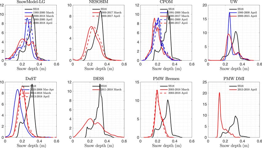
354                                                         L. Zhou et al.: Inter-comparison of snow depth over Arctic sea ice

Figure 4. Snow distribution comparison within the common regions (in Fig. 1a) in all snow products during the period 2000–2018 (different
products cover different periods) with/without DuST included in October–November (a, c) and March–April (b, d).

Figure 5. Snow distribution comparison between W 99 and snow products in spring (March and/or April).

The Cryosphere, 15, 345–367, 2021                                                            https://doi.org/10.5194/tc-15-345-2021
L. Zhou et al.: Inter-comparison of snow depth over Arctic sea ice                                                            355

Figure 6. Snow distribution comparison between SS18 climatology and snow products.

Figure 7. Time series of average monthly snow depth in each snow product within the common regions since 2000. Only wintertime
(September to next April) is shown.

cumulation is weakening or that the snow accumulation pe-          ther over the last 40 years, it is expected that the early snow
riod has shortened. We further note that W 99 accumulates          accumulation will continue to differ from that reflected in
more snow during the early part of winter, and thus the sea-       W 99.
sonal curves are flattened near spring. SnowModel-LG, NE-
SOSIM and CPOM on the other hand share similar seasonal            3.3   Trend and interannual variability of snow depth
accumulation curves, with accumulation continuing to in-
crease through winter. This seasonal pattern of winter snow        All reanalysis-based snow reconstructions, namely
accumulation finds support in a recent study by Kwok et al.        SnowModel-LG, CPOM, NESOSIM and UW, have
(2020) that found accumulation later in winter in 2018–2019.       consistent interannual variability in spring snow volume
This implies that there may be limited efficacy of the climato-    from 2000 to present (see details in Table S2), with statisti-
logical seasonal pattern of snow accumulation in the current       cally significant (confidence level 99 %) correlations of the
Arctic climate. As sea ice freeze-up continues to delay fur-       interannual snow depth/volume between the data sets. DESS
                                                                   also exhibits generally similar interannual variability to the

https://doi.org/10.5194/tc-15-345-2021                                                     The Cryosphere, 15, 345–367, 2021
356 L. Zhou et al.: Inter-comparison of snow depth over Arctic sea ice Figure 8. Wintertime snow accumulation among eight products and W 99 since 2000. reanalysis-based products (R 2 = 0.42 for SnowModel-LG, (Serreze et al., 2012) or changes in the proportion of MYI 0.68 for NESOSIM and 0.32 for CPOM), whereas PMW vs. FYI in the region. On the other hand, snow depth trends Bremen and DuST do not. in spring are mostly negative within the rest of the Arctic While there is interannual variability in snow accumula- basin and statistically significant for SnowModel-LG in FYI tion, the variability is overall quite small, ranging from 2 cm regions and for CPOM in the Barents Sea. In autumn, the re- in November to about 2 to 3 cm in April. This also holds gions with statistically significant negative snow depth trends for results as averaged up to 87.5◦ N (Fig. S3). The inter- in SnowModel-LG are larger, which is likely a result of de- annual variability seen in the data products is about half of lays in freeze-up (Markus et al., 2009; Stroeve and Notz, that previously reported in W 99, where interannual variabil- 2018). CPOM also shows negative trends in these regions ity was estimated to be about 4.3 cm in November and 6.1 cm but not as large as those from SnowModel-LG. April and in April. It is important to note, however, the climatological November mean snow depth trends from SnowModel-LG as estimation of interannual variability in W 99 includes snow computed over the entire Arctic basin are −0.5 and −0.9 cm depth uncertainties and should be treated as an upper bound per decade, respectively, although some regions show larger for the inherent physical interannual variability. It should be trends. In CPOM, a basin-mean significantly negative trend also noticed that DuST shows a significant positive snow (−0.47 cm decade−1 ) is only found in November. depth bias from the Envisat period to the CryoSat-2 period, Finally, we synthesize long-term changes in snow depth likely a result of using OIB to calibrate the snow depth es- in relationship to the climatology products. As mentioned in timates. This positive snow bias is missing in the passive- Sect. 3.1, the minimum and maximum differences of mean microwave-based snow products (e.g., PMW Bremen) and is snow depth in March and/or April between products in the not observed in DESS (time series in PMW DMI is too short current years and climatology are 10 and 15 cm respectively to be assessed). over the last 40 years; thus the inter-decadal snow depth As averaged over the common regions of all data sets, no changes would be in the range of −0.25 and −0.375 cm yr−1 . significant trend is observed in most snow products except These estimates span the value of −0.29 cm yr−1 in Webster DuST since 2000. However, regionally the reanalysis-based et al. (2014). However, one should keep in mind that there snow products exhibit regions of statistically significant pos- are large uncertainties in the snow climatology data sets, and itive and negative snow depth trends over a longer time the interannual variability is larger than in the snow products. period. For example, positive snow depth trends are found north of Greenland and the Canadian Arctic Archipelago from 1991 to 2015 (common period) (Fig. 9). These pos- itive trends may be a result of more autumn precipitation The Cryosphere, 15, 345–367, 2021 https://doi.org/10.5194/tc-15-345-2021
L. Zhou et al.: Inter-comparison of snow depth over Arctic sea ice 357
Figure 9. Trend of snow depth (units: cm yr−1 ) for SnowModel-LG, CPOM and UW in spring (April) (a–c) and autumn (November) (d, e)
during the period from 1991 to 2015. Areas with significant trends are shown as dotted areas (confidence level 95 %).
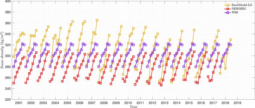
3.4 Snow density comparison ter; W 99 falls between the two estimates at 320 kg m−3 . Sea-
sonally, SnowModel-LG densities increase more from Octo-
ber to April than in NESOSIM and W 99. Neither the NE-
Apart from snow depth, we further investigate snow den- SOSIM nor SnowModel-LG densities suggest any long-term
sity in the two products that provide snow density estimates: changes in snow density, yet SnowModel-LG shows consid-
SnowModel-LG and NESOSIM. Since the W 99 climatol- erable interannual variability of spring and winter snow den-
ogy contains both snow depth and SWE, we can compare sity, which is not present in NESOSIM or W 99.
against the W 99 snow densities. Snow density in W 99 is lim-
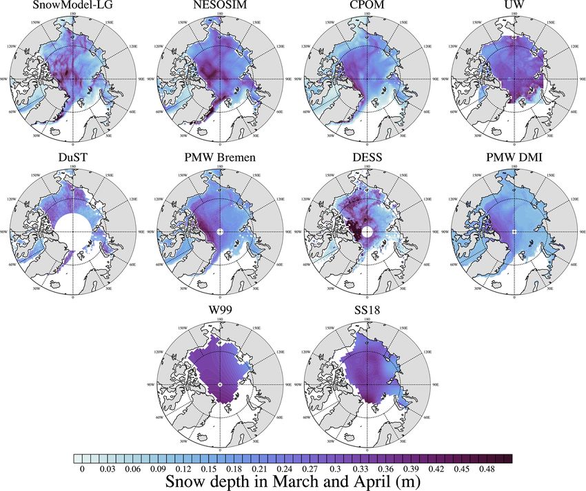
ited to the Arctic basin. SnowModel-LG suggests that snow
is denser than in NESOSIM in both November and April,
as shown in Fig. 10. Considering that the snow depth in 4 Comparison of snow depth products against
SnowModel-LG is thinner than NESOSIM, we find that the observations
two models provide a broadly equivalent SWE (not shown).
Snow over the Atlantic sector, especially within the East In this section, we compare the snow depth products against
Greenland Sea, is the densest in SnowModel-LG, with mean the observational data sets. Since snow depth data from OIB
density values above 370 kg m−3 in November and April. In play an important role in the development of some of the
contrast, NESOSIM has mostly smaller snow densities and snow products, the comparison and validation potentially
considerably less spatial variability. For W 99, the snow is suffer from the problem of data dependency. This applies to
denser over the Atlantic sector in November, while in April both reanalysis-based snow reconstructions and the satellite-
the denser snow is over the Pacific sector. retrieved snow depth fields. Buoy-based comparisons are free
Time series of wintertime mean snow density within from the data dependency problem, yet the limited local spa-
the Arctic basin in SnowModel-LG, NESOSIM and W 99 tial coverage of buoys hinders direct comparisons with the
are summarized in Fig. 11. Both SnowModel-LG and NE- products in study, which are all on much coarser spatial
SOSIM show an increase in snow density into the win- scales (> 10 km). Therefore, after the intercomparisons we
ter, which is consistent with W 99. However, snow density discuss the complexities in validating different snow prod-
in SnowModel-LG is consistently higher than that of NE- ucts and observations with in situ and airborne measurements
SOSIM, with more pronounced differences at the end of win- in Sect. 4.3.
https://doi.org/10.5194/tc-15-345-2021 The Cryosphere, 15, 345–367, 2021358 L. Zhou et al.: Inter-comparison of snow depth over Arctic sea ice
Figure 10. Mean snow density (units: kg m−3 ) according to SnowModel-LG, NESOSIM and W 99 in November (a–c) and the next April (d–
f) since 2000.
Figure 11. Time series of mean snow density (units: kg m−3 ) within Arctic basin (common region in Fig. 1) comparison in SnowModel-LG,
NESOSIM and W 99 since 2000.
4.1 Comparison against OIB measurement samples per grid cell. It should be noted that
snow depths from DuST, PMW Bremen and DMI are directly
We assess the snow products against four different OIB snow fitted against OIB snow depths, and as a result, these data
depth products. We first compare OIB and snow products af- show significantly correlations (over 0.36 for PMW DMI)
ter gridding both to a common 100 × 100 km grid and by with OIB as shown in Table 2. Therefore, we do not consider
evaluating the monthly averages in 2014 and 2015. Results this a suitable validation (or comparison) for these products.
are shown in Fig. 12 and Table 2. Taking the quicklook prod- For the PMW DMI product, however, OIB data from the pe-
uct as an example, there are on average 1300 OIB 40 m mean
The Cryosphere, 15, 345–367, 2021 https://doi.org/10.5194/tc-15-345-2021L. Zhou et al.: Inter-comparison of snow depth over Arctic sea ice 359 riod from March 2014–2015 were not used during model de- tween OIB and these products at the coarse scale of 100 km velopment, and hence we have more confidence in the high (discussed further in Sect. 4.3). correlation observed. Except for NESOSIM and UW, the Given the potential data dependency problem and the sen- other reanalysis-based products are also to some extent in- sitivity to the specific OIB data set, it is not possible to directly tuned by OIB snow depths in some years. Overall, conclude which snow product performs best. Snow products all products show reasonably high correlations with the dif- that have been produced through tuning with OIB data show ferent OIB snow estimates except for UW, which only shows higher R 2 and smaller RMSEs. The PMW DMI product per- a slight correlation with some versions of the OIB data. forms best, despite not being tuned with OIB data for the It should be noted that OIB snow depth is itself a de- time period to which it is compared. The outlier is the UW rived product, and thus caution is warranted when interpret- product. In summary, there is a need for a consensus as to ing the results of the comparison with snow products. In fact, which OIB data products are the most accurate and also for a strong dependence of our validation results on the specific further independent observations to compare against the var- OIB data product is evident by the different linear fitting ious pan-Arctic snow products currently available to the sci- slopes shown in Fig. 12, as well as the R 2 values, RMSE ence community. and normalized RMSE (NRMSE: RMSE/(max − min)) in Table 2. The fit is best for the PMW Bremen and PMW 4.2 Comparison with buoy data DMI data, followed by the CPOM and DESS products, though this depends on the choice of OIB data set used We further explore how well the snow products represent for evaluation. For example, CPOM performs best against the mean state of small-scale snow depth on Arctic sea ice SRLD (R 2 = 0.61) and worst against GSFC (R 2 = 0.43); by comparing against CRREL IMBs and AWI snow buoys. DESS also performs best against SRLD (R 2 = 0.59) but As discussed in Sect. 2.1.1, 86 buoy tracks (58 tracks are worst against quicklook (R 2 = 0.26). SnowModel-LG and from CRREL and 28 tracks are from AWI) were processed NESOSIM have similar R 2 ranging from a low R 2 of 0.27 from 2000 to 2017 (Table S1). Scatterplots in Fig. 13 be- and 0.29, respectively, against the quicklook product to a tween monthly mean (March and April) buoy snow depths high of 0.47 (SnowModel-LG vs. SRLD) and 0.39 (NE- and those from the various products are based on their na- SOSIM vs. GSFC). The UW snow product, on the other tive spatial resolution. DuST is excluded due to a lack of hand, performs poorly against all OIB snow depth estimates buoy samples in its more limited spatial coverage. Despite (maximum R 2 of 0.31 with SRLD). Among all non-directly some statistically significant correlations, the correlations are OIB-fitted snow products (SnowModel-LG, CPOM, DESS, all very low, with slopes close to 0. The highest correlation UW and NESOSIM), RMSE in CPOM is the lowest, while in among the products is 0.16 for DESS. The PMW Bremen and DESS the RMSE is over 10 cm. The distribution/variability PMW DMI products show essentially no variability/spread in UW is narrow compared with other products related to the compared to the buoy data. lack of spatial variability of snow depth across the basin. Next, we focus on temporal evolution as we do not ex- In order to avoid biases introduced by temporal and spa- pect the local-scale point measurements of the IMBs and tial averaging and interpolation during the validation, we also snow buoys to match with the coarse spatial scale of the carry out the comparison for each of the data products on data products. We compare snow depth differences in the their native grids and native temporal resolution (Fig. S4). products along the buoys’ drifting tracks against the accom- In contrast to the coarser-resolution comparisons shown in panied snow accumulation measured by buoys during win- Fig. 12 and Table 2, more outliers, lower R 2 values and ter (Fig. S5). Specifically, the three daily-resolution prod- larger RMSEs are evident in these native-spatial–temporal- ucts (SnowModel-LG, NESOSIM and CPOM) are inter- resolution comparisons. The comparison results still depend polated onto daily geolocations of the buoys. Only buoys on the choice of OIB data product, and in some instances with valid measurements from October until the follow- the statistical correlation improves. There is still no signif- ing February are considered. Snow accumulation is then icant correlation between UW snow depths and those from calculated by subtracting the mean snow depth within the OIB, but the overall RMSE is the lowest recorded at less first 7 d and that in the last 7 d. None of these products than 4.0 cm. PMW DMI has the lowest NRMSE, followed show significant correlation with buoy accumulation because closely by all other snow products, with the largest NRMSE several outliers weaken the overall correlation. Based on in DESS. All snow products except NESOSIM and UW Stroeve et al. (2020), good correlations are witnessed be- show higher R 2 under spatial coarser resolution compared tween SnowModel-LG and buoy data using the buoy location to Fig. 12, Fig. S4 and Table S3. The comparisons between in each integration step. Therefore, the lack of correlation we monthly and daily scale estimates suggests that temporal res- observe may be due to large discrepancies in trajectories de- olution has little influence on OIB comparisons, since there termined from the ice drift products and from buoys, espe- are only small changes in R 2 and RMSE, without significant cially after a long-term integration. differences. However, spatial resolution does impact the sta- In general, the comparison with snow depth measure- tistical fits, which is related to the lack of representation be- ments from buoys highlights two important limitations of https://doi.org/10.5194/tc-15-345-2021 The Cryosphere, 15, 345–367, 2021
You can also read