Baseline Surveys for Seabirds in the Labrador Sea Relevés de référence sur les oiseaux marins dans la mer du Labrador 206
←
→
Page content transcription
If your browser does not render page correctly, please read the page content below
Environmental
      Studies
      Research
      Fund

206

   Baseline Surveys for Seabirds in the
   Labrador Sea

   Relevés de référence sur les oiseaux
   marins dans la mer du Labrador

                                          \

Canada                     March 2016
Correct citation for this report is:

D. A. Fifield, A. Hedd, G. J. Robertson, S. Avery‐Gomm, C. Gjerdrum, L. A. McFarlane Tranquilla, S. J.
Duffy. 2016. Baseline Surveys for Seabirds in the Labrador Sea (201‐08S). Environmental Studies
Research Funds Report No. 206. St. John’s. 69 pp.
Environmental Studies Research Funds

Baseline Surveys for Seabirds in the Labrador Sea
                    (201‐08S)

                    Final Report

                 Wildlife Research Division
          Environment and Climate Change Canada
                 St. John’s, Newfoundland

                       March 2016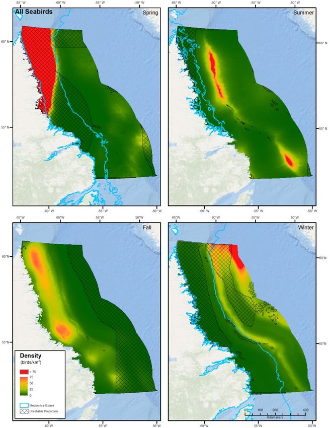
Baseline Surveys for Seabirds in the Labrador Sea Final Report

Acknowledgements

We thank the Environmental Studies Research Funds (ESRF) for funding support and Dave Burley of
the Canada‐Newfoundland and Labrador Offshore Petroleum Board (C‐NLOPB) and Dave Taylor
(ESRF Secretariat) for guidance and support throughout. Access to survey vessels was kindly
provided in part by DFO chief scientists, and CCGS captains. Environment and Climate Change
Canada (ECCC) management and administrative support was provided by Kevin Cash, Richard Elliot,
François Fournier and Don Moncrieff. We thank Jack Lawson (DF0) for the opportunity to
participate in aerial surveys and for fruitful discussion of survey and analysis methods. We thank the
Nunatsiavut Government and NunatuKavut for support and participation in the observer training
workshop. We also thank the many dedicated observers who spent long hours collecting data in
often less than ideal weather conditions, and the captains and crews for their hospitality. Alejandro
Buren, Francois Bolduc, Pat O’Hara, Rob Ronconi, Pierre Ryan, Sabina Wilhelm and Sarah Wong
contributed to many discussions of survey techniques, analysis and mapping.

                                                                                                    i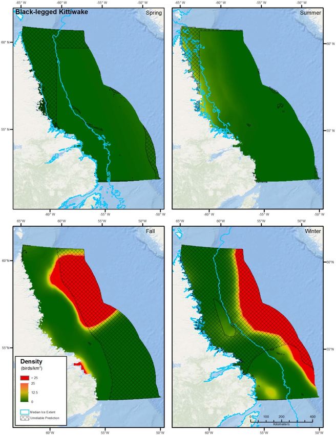
Baseline Surveys for Seabirds in the Labrador Sea Final Report

Table of Contents

Acknowledgements................................................................................................................................. i
Table of Contents ................................................................................................................................... ii
List of Figures ........................................................................................................................................ iv
List of Tables........................................................................................................................................... v
1      Executive summary ........................................................................................................................1
2      Introduction ................................................................................................................................... 2
3      Objectives ...................................................................................................................................... 3
4      Methods......................................................................................................................................... 4
  4.1    Study Area ............................................................................................................................... 4
  4.2    Ship‐based surveys .................................................................................................................5
  4.3    Aerial surveys ..........................................................................................................................6
  4.4    Ship‐based data analysis ......................................................................................................... 8
     4.4.1     Data extraction and filtering ........................................................................................... 8
     4.4.2     Modeling approach ......................................................................................................... 9
     4.4.3     Mapping of results ........................................................................................................16
     4.4.4     Seasonal density estimates ........................................................................................... 16
5    Results.......................................................................................................................................... 17
  5.1    Objective 1. Conduct baseline surveys of seabirds in the Labrador Sea in support of
  ongoing oil and gas exploration and future oil and gas development ............................................17
     5.1.1     Ship‐based Surveys .......................................................................................................17
     5.1.2     Aerial Surveys ................................................................................................................23
  5.2    Objective 2. To identify, collate, and integrate any existing data relevant to pelagic seabird
  distributions in the Labrador Sea .....................................................................................................26
  5.3    Objective 3. To provide fundamental information on the distribution and population
  densities of the seabirds in the study area ...................................................................................... 26
     5.3.1     Raw results ....................................................................................................................26
     5.3.2     Detection function models............................................................................................ 26
     5.3.3     Densities ........................................................................................................................26
  5.4    Objective 4. To involve, train, and transfer expertise to local and in particular, indigenous
  individuals, the technical skills involved in conducting such surveys whenever possible ............... 32
  5.5    Objective 5. To maintain positive control of the scientific methodology and quality of the
  data gathered during the surveys .................................................................................................... 34
  5.6    Objective 6. To ensure safety of any in‐field study operations ............................................35
6    Discussion and Recommendations .............................................................................................. 35
    6.1       Importance of the Labrador Sea ........................................................................................... 35
    6.2       Use of predictive density surface modeling.......................................................................... 35
    6.3       Remaining gaps .....................................................................................................................36
    6.4       Aerial surveys ........................................................................................................................37

    6.5       Integration of industry collected data .................................................................................. 37
                                                                                                                                         ii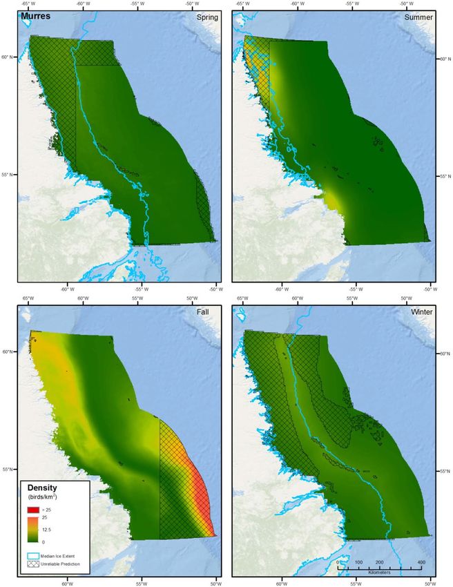
Baseline Surveys for Seabirds in the Labrador Sea Final Report
7    Literature Cited ............................................................................................................................ 39
8      Appendices .................................................................................................................................. 43
    8.1    Appendix 1. Seabird density maps........................................................................................ 43
       8.1.1   All seabirds ....................................................................................................................44
       8.1.2   Atlantic puffin................................................................................................................46
       8.1.3   Black‐legged kittiwake .................................................................................................. 48
       8.1.4   Dovekie..........................................................................................................................50
       8.1.5   Gulls............................................................................................................................... 52
       8.1.6   Murres ...........................................................................................................................54
       8.1.7   Northern fulmar ............................................................................................................56
       8.1.8   Shearwaters ..................................................................................................................58
    8.2    Appendix 2: Summary of recommendations stemming from this report ............................ 60

                                                                                                                                                     ii
Baseline Surveys for Seabirds in the Labrador Sea Final Report

List of Figures

Figure 1. Labrador Sea study area, which encompasses the area of the Labrador Sea delineated by
        NAFO regions 2G, 2H, 2J, out to the Canadian EEZ (Exclusive Economic Zone). Significant
        discovery licenses and active C‐NLOPB land issuance sectors in the Labrador Sea are also
        indicated. ................................................................................................................................... 5
Figure 2. Typical histogram of observed distances with fitted detection function (smooth black
        curve). For our study the distance categories were A: 0‐50m, B: 50‐100m, C:100‐200m,
        D:200‐300m. The detection probability, labeled “Correction Factor” here is computed as the
        area under the curve divided by the area of the dashed rectangle. Adapted from Gjerdrum
        et al. (2012).............................................................................................................................. 11
Figure 3. Example plots of 3 smooth terms employed in a Generalized Additive Model (GAM) that
        show the seasonal effect of distance to the 1000 m isobath on bird density that were A)
        retained in the model (Atlantic puffin), B) replaced with a parametric term (gulls), and C)
        removed from the model (gulls). .............................................................................................13
Figure 4. Survey effort (2006‐2008, 2011‐2014) including ECSAS surveys (red), and those supported
        by ESRF during this study or previously (yellow) that were completed specifically to address
        the data gap in the Labrador Sea............................................................................................. 21
Figure 5. Seasonal ship‐based survey effort (2006‐2008, 2011‐2014) in Labrador Sea. ...................... 22
Figure 6. Participants in the Seabird and Marine Mammal Observer Training workshop in Happy‐
        Valley Goose Bay 13‐14 November 2014. ...............................................................................34
Figure 7. Seasonal predicted densities (2 km x 2 km grid) of all seabirds based on Generalized
        Additive Models (GAMs).......................................................................................................... 44
Figure 8. Seasonal bird observations and coefficient of variation (CV, 6 km by 6 km grid) for
        predicted densities of all seabirds based on Generalized Additive Models (GAMs). .............. 45
Figure 9. Seasonal predicted densities (2 km x 2 km grid) of Atlantic puffin based on Generalized
        Additive Models (GAMs).......................................................................................................... 46
Figure 10. Seasonal bird observations and coefficient of variation (CV, 6 km by 6 km grid) for
        predicted densities of Atlantic puffin based on Generalized Additive Models (GAMs). ......... 47

                                                                                                                                                     iv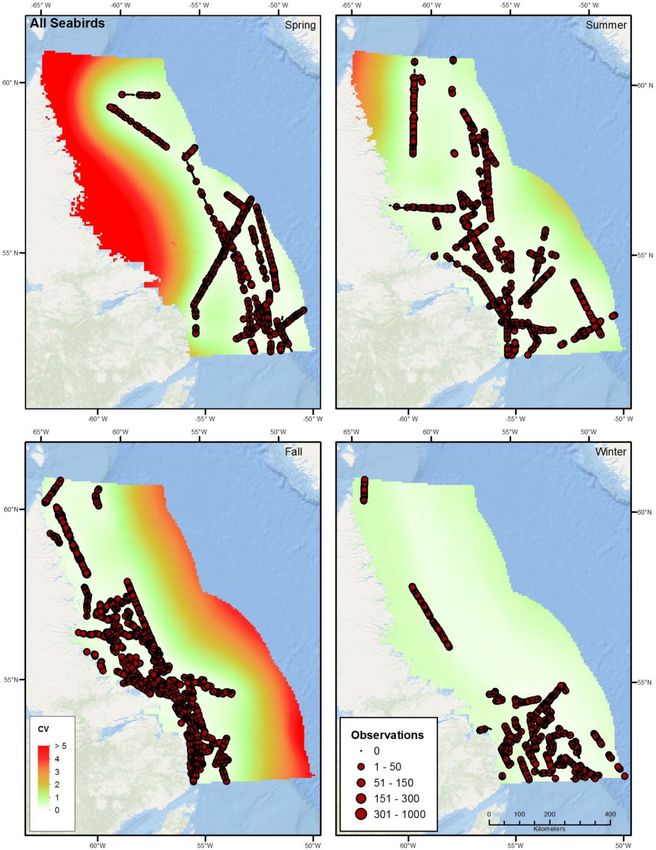
Baseline Surveys for Seabirds in the Labrador Sea Final Report
Figure 11. Seasonal predicted densities (2 km x 2 km grid) of Black‐legged kittiwake based on
Generalized Additive Models (GAMs). ....................................................................................48
Figure 12. Seasonal bird observations and coefficient of variation (CV, 6 km by 6 km grid) for
predicted densities of Black‐legged kittiwake based on Generalized Additive Models (GAMs).
.................................................................................................................................................49
Figure 13. Seasonal predicted densities (2 km x 2 km grid) of dovekie based on Generalized Additive
Models (GAMs). ....................................................................................................................... 50
Figure 14. Seasonal bird observations and coefficient of variation (CV, 6 km by 6 km grid) for
predicted densities of dovekie based on Generalized Additive Models (GAMs). ................... 51
Figure 15. Seasonal predicted densities (2 km x 2 km grid) of gulls based on Generalized Additive
Models (GAMs). ....................................................................................................................... 52
Figure 16. Seasonal bird observations and coefficient of variation (CV, 6 km by 6 km grid) for
predicted densities of gulls based on Generalized Additive Models (GAMs) ......................... 53
Figure 17. Seasonal predicted densities (2 km x 2 km grid) of murres based on Generalized Additive
Models (GAMs). ....................................................................................................................... 54
Figure 18. Seasonal bird observations and coefficient of variation (CV, 6 km by 6 km grid) for
predicted densities of murres based on Generalized Additive Models (GAMs). .................... 55
Figure 19. Seasonal predicted densities (2 km x 2 km grid) of Northern fulmar based on Generalized
Additive Models (GAMs). ........................................................................................................ 56
Figure 20. Seasonal bird observations and coefficient of variation (CV, 6 km by 6 km grid) for
predicted densities of Northern fulmar based on Generalized Additive Models (GAMs) ...... 57
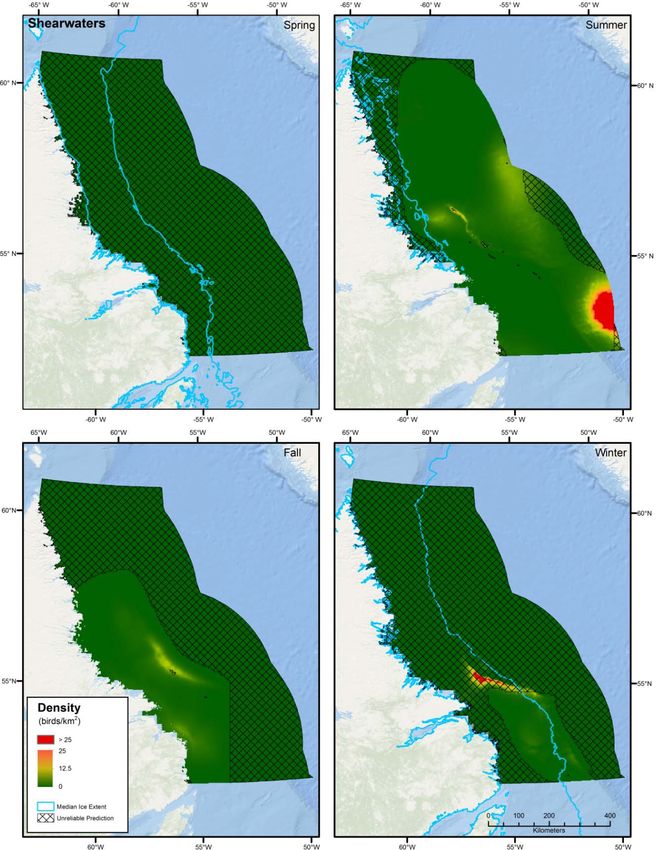
Figure 21. Seasonal predicted densities (2 km x 2 km grid) of shearwaters based on Generalized
Additive Models (GAMs). ........................................................................................................ 58
Figure 22. Seasonal bird observations and coefficient of variation (CV, 6 km by 6 km grid) for
predicted densities of shearwaters based on Generalized Additive Models (GAMs) ............. 59
List of Tables
Table 1. Environmental variables collected during ship‐based surveys. ............................................... 6
Table 2. Distance categories for aerial and ship‐based surveys, and clinometer angles used for aerial
surveys for aircraft flying at a nominal 600’. .............................................................................8
v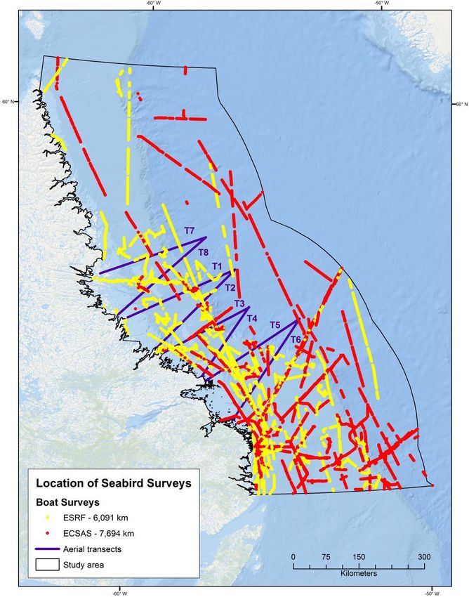
Baseline Surveys for Seabirds in the Labrador Sea Final Report

Table 3. List of eight seabird guilds analyzed for this report. ................................................................ 9
Table 4. List of environmental variables used to model the density of seabirds within the Labrador
          Sea. .......................................................................................................................................... 15
Table 5. Details of 35 survey trips whose data are analyzed in this report. Surveys supported by the
          ESRF during this study (or previously) are highlighted in bold. ...............................................18
Table 6. Vessel‐survey effort and data used for density surface models of seabirds within the
          Labrador Sea, summarized by collection year, season and program ...................................... 20
Table 7. Summary of species sighted from Labrador Sea aerial surveys, from 16‐17 October and 7
          November, 2013. ..................................................................................................................... 24
Table 8. Summary of species sighted from Labrador Sea aerial surveys, from 25, 26, and 28 August,
          2014. ........................................................................................................................................ 25
Table 9. Detection function models for each guild. ............................................................................. 27
Table 10. Density surface models for each guild.................................................................................. 28

                                                                                                                                                         vi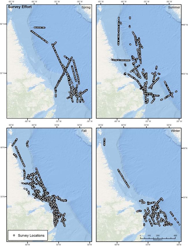
Baseline Surveys for Seabirds in the Labrador Sea Final Report

1   Executive summary
The Labrador Sea is important to marine birds year‐round, by supporting breeding seabird colonies
during summer, and providing important staging, migration, and wintering habitat for seabirds from
widespread colonies across the Atlantic. However, explicit local‐scale spatial information on marine
bird distribution has been limited by patchy marine survey coverage in the Labrador Sea, mostly
due to logistical difficulties. To fill this gap, baseline data on seabird distribution were collected
from vessels and aerial surveys in Labrador in 2013 and 2014. These data were combined with data
from Environment and Climate Change Canada’s Eastern Canada Seabirds At Sea (ECSAS) program,
(funded in part by ESRF 2006‐2009) to take advantage of new analysis methods in species
distribution modeling to provide a richer description of seabird densities and distributions in the
Labrador Sea.

From May 2006 to November 2014, ECSAS observers surveyed 13783.3 linear km (over 713 h) for
seabirds within the Labrador Sea study area, with the most intensive effort occurring between 2012
and 2014. Surveys were conducted during all seasons, however, as survey platforms were largely
ships of opportunity, effort was distributed unevenly across the study area through time. In total,
ship surveys yielded 33,469 seabirds detected (12,379 flocks during 13783.3 km of transects, Table
6) in 4638 of 8392 (55%) survey segments, with dovekie, northern fulmar, black‐legged kittiwake,
and murres being most frequently observed. Average detection probability was 38% (CV=0.26) for
all seabirds combined, ranging from a low of 31% (CV = 0.03) for dovekie to 54% (CV = 0.11) for
Atlantic puffin. Density surface modelling efforts were generally successful, although depending on
the species and season, reasonable predictions of seabird density were not possible for significant
portions of the study area. Models explained between 21.7% and 68.3% of the deviance in the data,
and position (latitude and longitude), sea surface temperature, sea surface height, bathymetry,
distance to the shelf edge and eddy kinetic energy were important predictors in most models.

The Labrador Shelf and adjacent portions of the Labrador Sea were clearly important regions for
seabirds, particularly during fall and winter, when average densities in areas of acceptable precision
were 15.5 and 12.8 birds/km2, respectively. During fall, relatively high densities were predicted
throughout the Labrador Shelf, from the Saglek and Nain Banks south to the Labrador Trough,
overlapping with areas of significant discovery licenses and coincident with southward migration of
dovekies and murres from Arctic breeding colonies. Northern fulmars had the highest predicted
densities in fall and winter (29.8 and 62.9 birds/km2), followed by Black‐legged Kittiwakes (13.8 and
20.6 birds/km2), although confidence intervals were large for these species. Dovekies (17.1 and 14.8
birds/km2) and murres (4.9 and 2.2 birds/km2) were also numerous in fall and winter, and modeling
efforts for these two species, especially murres, led to reasonable prediction throughout much of
the study area. Gulls, Atlantic puffins and shearwaters were present in the study area at lower
densities.

In conjunction with the DFO marine mammal surveys, four exploratory aerial surveys (2 in Oct‐Nov
2013 and 2 in Aug 2014) were conducted to develop methods compatible with marine mammal
observation protocols. 6,301 marine birds were counted in the 2013 surveys and 4,346 in the 2014
surveys. Northern fulmars were the most commonly detected seabird, followed by common eiders
and unidentified alcids, with gulls making up the bulk of the remaining observations. The altitude of

                                                                                                   1
Baseline Surveys for Seabirds in the Labrador Sea Final Report
these particular surveys (600 ft) was too high for reliable seabird observations, and many birds
could not be identified to species, limiting the utility of them for seabirds.
On 13‐14 November 2014 ECCC and DFO taught a Seabird and Marine Mammal Observer Training
workshop in Happy‐Valley Goose Bay. The workshop had 20 attendees from 6 communities (Port
Hope Simpson, North West River, Happy Valley‐Goose Bay, Hopedale, Makkovik and Nain)
representing a diverse range of experience. Despite the diverse background of attendees (55%
arrived with limited understanding of the subject), 90% reported that the workshop was extremely
useful.
In consultation with researchers, C‐NLOPB and industry, 21 existing seabird surveys occurring in the
Labrador Sea were identified. Of these 9 were useable and imported into the ECSAS database. The
others could or were not used for various reasons including survey protocol incompatibility (for
industry surveys, because the ECSAS protocol was not published until 2012 and not provided to the
C‐NLOPB until the spring of 2015), and unavailability of data.
Overall, this program was successful in improving knowledge of seabird distribution and densities in
the Labrador Sea. Although the density surface modeling proved very powerful in expanding the
geographic scope of prediction beyond the available data, gaps in survey coverage remain,
particularly off the continental shelf in fall and winter, and in the northern portion of the study area
in all seasons. Future work should consider filling those seasonal and spatial gaps, and continuing to
improve density surface modeling efforts, both in the Labrador Sea, in adjacent regions of interest
to the offshore oil and gas industry.
The data analyzed in this report are available from Dave Fifield (dave.fifield@canada.ca) at
Environment and Climate Change Canada.
Sommaire
La mer du Labrador est importante pour les oiseaux marins toute l’année : l’été, elle soutient les
colonies reproductrices d’oiseaux marins et l’hiver, elle offre un habitat important d’escale, de
migration et d’hivernage aux oiseaux marins de colonies répandues sur tout l’Atlantique. Or, il y a
une lacune de données spatiales explicites à l’échelle locale sur la répartition des oiseaux marins en
raison de la couverture irrégulière des relevés marins effectués dans la mer du Labrador, surtout à
cause de difficultés logistiques. Pour combler cette lacune, des données de base sur la répartition
des oiseaux marins ont donc été recueillies à partir de navires et de levés aériens au Labrador en
2013 et 2014. Ces données et des données du programme Eastern Canada Seabirds at Sea (oiseaux
en mer dans l’est du Canada) ou ECSAS (partiellement financés par le Fonds pour l’étude de
l’environnement de 2006 à 2009) ont été mises ensemble afin de profiter de nouvelles méthodes
d’analyse dans la modélisation de la répartition des espèces pour avoir une description plus riche
de la densité des oiseaux marins et de leur répartition dans la mer du Labrador.
De mai 2006 à novembre 2014, des observateurs du programme ECSAS ont effectué un relevé des
oiseaux marins dans la zone d’étude de la mer du Labrador, couvrant 13 783,3 km linéaires (sur
713 heures), dont les efforts les plus intenses ont eu lieu entre 2012 et 2014. Les relevés ont été
effectués pendant toutes les saisons, mais puisque ce sont des navires occasionnels qui servent
2Baseline Surveys for Seabirds in the Labrador Sea Final Report
normalement de plateforme pour les relevés, pendant la période d’étude, la répartition des efforts
était inégale dans l’ensemble de la zone d’étude. Les relevés des navires ont permis de détecter
33 469 oiseaux marins (12 379 bandes sur 13 783,3 km de transects; Tableau 6) dans 4 638 des
8 392 segments (55 %), dont les plus fréquemment observés étaient le mergule nain, le fulmar
boréal, la mouette tridactyle et les guillemots. Pour l’ensemble des oiseaux de mer, la probabilité
de détection moyenne était 38 % (CV=0,26), allant d’une faible probabilité de 31 % (CV = 0,03) pour
le mergule nain à 54 % (CV = 0,11) pour le macareux moine. En général, les efforts de modélisation
de la densité de surface ont été réussis. Toutefois, selon l’espèce et la saison, il n’était pas possible
de faire des prévisions raisonnables quant à la densité des oiseaux marins dans des parties
importantes de la zone d’étude. Les modèles ont expliqué de 21,7 à 68,3 % de l’écart dans les
données, et dans la plupart des modèles, la position (latitude et longitude), la température de la
surface de la mer, la hauteur de la mer, la bathymétrie, la distance jusqu’au bord du plateau
continental et l’énergie de turbulence était des prédicteurs importants.
Le plateau continental du Labrador et les parties adjacentes de la mer du Labrador étaient
manifestement des régions importantes pour les oiseaux marins et en particulier, à l’automne et
l’hiver alors que les densités moyennes étaient de 15,5 et de 12,8 oiseaux/km2, respectivement,
dans les zones où la précision était acceptable. À l’automne, des densités relativement élevées ont
été prévues pour l’ensemble du plateau continental du Labrador, des bancs Saglek et Nain vers le
sud jusqu’à la fosse du Labrador, chevauchant des zones importantes de licence de découverte
importante et coïncidant avec la migration vers le sud de populations de mergule nain et de
guillemot de leurs colonies de reproduction dans l’Arctique. À l’automne et l’hiver, les densités
prévues des fulmars boréaux étaient les plus élevées (29,8 et 62,9 oiseaux/km2), suivies de celles
des mouettes tridactyles (13,8 et 20,6 oiseaux/km2), quoique les intervalles de confiance soient
larges pour ces espèces. Les mergules nains (17,1 et 14,8 oiseaux/km2) et les guillemots (4,9 et
2,2 oiseaux/km2) étaient également nombreux à l’automne et l’hiver et les efforts de modélisation
des deux espèces, surtout des guillemots, ont permis de faire des prévisions raisonnables pendant
une grande partie de la zone d’étude. Les mouettes et les goélands, les macareux moines et les
puffins étaient présents dans la zone d’étude à des densités plus faibles.
De pair avec les relevés de mammifères marins effectués par Pêches et Océans Canada, quatre
levés aériens de reconnaissance (deux en octobre et novembre 2013 et deux en août 2014) ont été
effectués afin d’élaborer des méthodes compatibles avec les protocoles d’observation des
mammifères marins. Lors des relevés en 2013 et en 2014, 6 301 et 4 346 oiseaux marins ont été
comptés, respectivement. L’oiseau marin le plus souvent détecté était les fulmars boréaux, suivis
des eiders à duvet et des alcidés non identifiés. Les mouettes et goélands composaient les autres
observations pour la plupart. L’altitude à laquelle ces relevés ont été effectués (600 pi) était trop
haute pour faire des observations fiables sur les oiseaux marins et l’espèce de nombreux oiseaux
n’a pu être identifiée, ce qui a rendu moins utiles ces observations.
Le 13 et 14 novembre 2014, Environnement et Changement climatique Canada et Pêches et Océans
Canada ont tenu un atelier de formation sur l’observation d’oiseaux et de mammifères marins à
Happy-Valley Goose Bay, au Labarador. L’atelier comptait 20 participants de six communautés (Port
Hope Simpson, North West River, Happy Valley-Goose Bay, Hopedale, Makkovik et Nain),
représentant une vaste gamme d’expérience. Malgré les antécédents divers des participants (55 %
avaient une compréhension limitée du sujet de l’atelier), 90 % d’entre eux ont dit que l’atelier a été
extrêmement utile.
3Baseline Surveys for Seabirds in the Labrador Sea Final Report
En consultation avec des chercheurs, l’Office Canada-Terre-Neuve des hydrocarbures extracôtiers
et l’industrie, 21 relevés d’oiseaux marins présents dans la mer du Labrador ont été trouvés. De ces
relevés, neuf étaient utiles et ils ont été importés dans la base de données du programme ECSAS.
Les autres relevés n’ont pas été utilisés pour diverses raisons, notamment l’incompatibilité du
protocole d'enquête (pour les enquêtes de l'industrie, parce que le protocole ECSAS n'a été publié
qu'en 2012 et non fourni à l'OCTLHE jusqu'au printemps 2015) et la non-disponibilité de données.
Globalement, ce programme a réussi à accroître les connaissances sur la répartition et les densités
des oiseaux marins dans la mer du Labrador. La modélisation de la densité de surface s’est avérée
très efficace pour élargir l’étendue géographique de prévision au-delà des données existantes, mais
des écarts demeurent quant à la couverture des relevés et en particulier, au large du plateau
continental à l’automne et l’hiver et dans la partie nord de la zone d’étude toute l’année. Pour les
travaux à l’avenir, il est recommandé de considérer ce qui suit : combler les écarts saisonniers et
spatiaux; continuer à améliorer les efforts de modélisation de la densité de surface, dans la mer du
Labrador et dans les régions d’intérêt adjacentes à l’industrie pétrolière et gazière extracôtière.
Pour consulter les données analysées dans le rapport ci-dessus, veuillez prendre contact avec Dave
Fifield (dave.fifield@canada.ca) à Environnement et Changement climatique Canada.
2 Introduction
The Labrador Sea is important to marine birds year‐round, by supporting breeding seabird colonies
during summer, and providing important staging, migration, and wintering habitat for seabirds from
widespread colonies internationally, including Canada, Greenland, Iceland, Svalbard, and the UK
(Brown 1986, Huettmann and Diamond 2000, Bakken and Mehlum 2005, Frederiksen et al. 2012,
Mosbech et al. 2012, Jessopp et al. 2013, Linnebjerg et al. 2013, Fort et al. 2013, McFarlane
Tranquilla et al. 2013). However, explicit local‐scale spatial information on marine bird distribution
has been limited by patchy marine survey coverage in the Labrador Sea (Fifield et al. 2009), mostly
due to logistical difficulties.
The Labrador Sea contains significant oil and gas reserves and has been a focus for resource
exploration for decades (AMAP 2010). Yet, only recently has an increase in interest for offshore
exploration in the Labrador Sea prompted a demand for better baseline biological data, currently
sparse in this region (Fifield et al. 2009), required to support regional scale environmental
assessments (C‐NLOPB 2008). Seabirds are extremely vulnerable to the effects of oil at sea (Wiese
and Robertson 2004, O’Hara and Morandin 2010), but determining the effect of an accidental
hydrocarbon release in the marine environment is difficult when seabird densities in a particular
area, and a particular season, are not known (Wilhelm et al. 2007).
4Baseline Surveys for Seabirds in the Labrador Sea Final Report
Understanding the spatial and temporal extent of overlap of marine bird populations with offshore
resource activities will be critical to the environmental assessment process (Camphuysen et al.
2004, Fifield et al. 2009), and to understanding potential risks to marine birds.
Since 2006 Environment and Climate Change Canada (ECCC) has developed a rigorous seabird at sea
monitoring program for eastern Canada, known as the ECSAS (Eastern Canada Seabirds At Sea)
program. This program has developed standardized protocols, a sophisticated data entry and
management system, an inventory of required equipment (field‐ready laptops and optics), training
materials, a pool of qualified seabird observers with necessary safety training and analytical
expertise in survey data analysis (with a specific focus on DISTANCE sampling). Previously funded
ESRF projects, specifically the Offshore Seabird Monitoring Program (ESRF Report Number of 183;
Fifield et al. 2009), which focused on areas of current production in Atlantic Canada, helped to
move forward on many of these program components. All of these resources were available and
required to initiate this study of seabird distributions in the Labrador Sea.
To portray seabird densities across Atlantic Canada waters, Fifield et al. (2009) presented means
and variances for each species‐group in 1° blocks of latitude and longitude. Although valid, this
approach has some drawbacks, including the possibility of limited data in each block, the lack of any
relationship in densities between adjacent blocks and the lack of use of any oceanographic or
biological data that may help to understand drivers of seabird distributions and densities. Recent
statistical advances in species distribution modeling (SDM), or density surface modeling (DSM), are
providing an emerging framework that overcomes many of the constraints of the previous analysis
(Miller et al 2013). Survey data are used directly to examine relationships between environmental
covariates (generally collected by remote sensing) and seabird densities. Once these relationships
are understood, predictions of seabird densities to areas of comparable environmental conditions
are possible – even when there is no survey coverage in the immediate area (although predictions
do become weaker as environmental conditions and distance from the surveyed area increases).
These statistical approaches are an active area of research (Miller et al. 2013, Hedley et al. 2004),
but all are based on advanced techniques and extensive experience and training are required.
This report, supported by ESRF, details the collection of baseline data on seabird distributions in the
Labrador Sea that could be affected by offshore activities. We take advantage of new analysis
methods in species distribution modeling to provide a richer description of seabird densities and
distributions in the Labrador Sea. These methods include distance sampling analysis (Miller 2015,
Buckland et al. 2001) of data collected with an appropriate protocol (Gjerdrum et al. 2012) coupled
with density surface modelling of abundance (Miller et al. 2015, Miller 2013). See also the
companion report, Lawson et al. (2016), for a similar modelling exercise of marine mammal
occurrence in the Labrador Sea.
3 Objectives
As stated in the MOU, this project supports baseline surveys of seabirds in the Labrador Sea, in
order to provide information that will support regulatory decision‐making regarding mitigation of
the effects of oil and gas production activities in the Labrador Sea (Figure 1).
5Baseline Surveys for Seabirds in the Labrador Sea Final Report
The specific objectives of this study are to :
1. Conduct baseline surveys of seabirds in the Labrador Sea in support of ongoing oil and gas
exploration and future oil and gas development;
2. To identify, collate, and integrate any existing data relevant to pelagic seabird distributions
in the Labrador Sea;
3. To provide fundamental information on the distribution and species population densities of
the seabirds in the study area;
4. To involve, train, and transfer expertise to local and in particular, indigenous individuals, the
technical skills involved in conducting such surveys whenever possible;
5. To maintain positive control of the scientific methodology and quality of the data gathered
during the surveys;
6. To ensure safety of any in‐field study operations
4 Methods
4.1 Study Area
The study area is aligned with the Labrador Shelf Strategic Environmental Assessment (SEA) Area (C‐
NLOPB 2008), defined using NAFO regions (2G, 2H, 2J) within the Canadian EEZ.
6Baseline Surveys for Seabirds in the Labrador Sea Final Report
Figure 1. Labrador Sea study area, which encompasses the area of the Labrador Sea delineated by
NAFO regions 2G, 2H, 2J, out to the Canadian EEZ (Exclusive Economic Zone). Significant discovery
licenses and active C‐NLOPB land issuance sectors in the Labrador Sea are also indicated.
4.2 Ship‐based surveys
Surveys were conducted within the purview of Canadian Wildlife Service’s ongoing Eastern Canada
Seabirds At Sea (ECSAS) program (Gjerdrum et al. 2012), benefitting from access to a pool of
experienced observers, established logistical support, and the strength of an ongoing database
archive. Ship‐based surveys were conducted following a standardized protocol that incorporates
Distance Sampling methods (Gjerdrum et al. 2012, Buckland et al. 2001).
7Baseline Surveys for Seabirds in the Labrador Sea Final Report
Observers were placed on ships of opportunity, except for four surveys that were contracted
directly with funds from ESRF. Three were in the Labrador Sea; two in 2013 and 2014 aboard the
F/V What’s Happening from Nain, Labrador, captained by Mr. Joey Agnatok and one trip in 2015
aboard the F/V Labrador Venture from L’Anse au Loup, Labrador, captained by Mr. Lloyd Normore.
These cruises were primarily intended to deploy and retrieve hydroacoustic recorders at two points
on the Labrador Shelf to detect marine mammals (in collaboration with Dr. Jack Lawson, DFO; see
MOU “Mid‐Labrador Marine Megafauna and Acoustic Surveys on the Labrador Coast (2010‐07S)”
and associated report). The fourth survey was part of an Arctic Biodiversity Survey aboard the M/V
Cape Race led by the University of New Brunswick. This cruise steamed from Qikiqtarjuaq, Nunavut
south along the entire Labrador coast, to St. Pierre et Miquelon in September of 2014. The vessel
charter was cost‐shared with the University of New Brunswick, University of Guelph, Université de
Laval, University of Toronto, University of Rhode Island, the Smithsonian, and Parks Canada.
Ship‐based surveys were conducted using distance sampling (Buckland et al. 2001) according to the
ECSAS protocol (Gjerdrum et al. 2012) and are explained more fully in Fifield et al. (2009). Briefly,
surveys consisted of nominally 5‐minute observation periods (called segments) along a continuous
transect line. Coordinates at the beginning and end of each segment were recorded using ship‐
based navigation systems, puck‐style GPS’s, or with hand‐held GPS units. Environmental variables
were collected and updated at the beginning of each segment (Table 1; see also Gjerdrum et al.
2012). We recorded birds on the water continuously along each segment, but we used a snapshot
approach for flying birds (Tasker et al. 1984, Gjerdrum et al. 2012). Distance categories (see Table 2)
were assigned by measuring the perpendicular distance to each individual bird (or the centroid of
each group of birds) with the help of a pre‐marked custom ruler constructed for each observer‐
vessel combination (Gjerdrum et al. 2012). Data was either entered directly into the ECSAS
Microsoft Access database using voice recognition software, or recorded on datasheets and entered
into the database later (see full details in Fifield et al. 2009).
Table 1. Environmental variables collected during ship‐based surveys.
Variable Name
Visibility (km)
Weather code
Glare conditions code
Sea state code
Wave height (m)
True wind speed (knots) OR Beaufort scale
True wind direction (deg)
Ice type code
Ice concentration code
4.3 Aerial surveys
The existence of aerial marine mammal surveys in the Labrador Sea (“Mid‐Labrador Marine
Megafauna and Acoustic Surveys on the Labrador Coast (2010‐07S)”(Lawson et al. 2016), led by Dr.
Jack Lawson, DFO) gave us the opportunity to collaborate and attempt to survey marine birds in
2013 and 2014. The survey route, altitude, and speed were pre‐determined by the marine mammal
8Baseline Surveys for Seabirds in the Labrador Sea Final Report
survey protocol and we developed a specific aerial survey protocol in this context. Surveys were
flown at a nominal flight speed of 100 knots at an altitude of 600 feet using a Twin Otter aircraft
operated by Air Labrador based out of Happy Valley‐Goose Bay, Newfoundland and Labrador.
Cross‐shelf transects were designed to capture variation in marine mammal (and seabird)
distribution across a variety of depths and to ensure survey coverage beyond the shelf edge. Flight
path and direction were chosen to ensure proximity to airstrips and fuel throughout the duration of
the survey for logistical and safety considerations.
In 2013, data were collected by two seabird observers from both the port and starboard sides
simultaneously, with observers switching positions at regular intervals during replicate 1 and
remaining on the same side during the entirety of replicate 2 (see Results). In 2014, both seabird
observers were seated on the port side. Two types of window (bubble and flat) were tested. Bubble
windows allowed observers to see directly below the aircraft while flat windows occlude this part of
the transect. In 2013, the port observer used a bubble window while a flat window was used on the
starboard side. In 2014, the front observer was equipped with a large bubble window and a smaller
one was used in the rear of the aircraft.
Aerial surveys were conducted using distance sampling where perpendicular distance is measured
from the survey line to detected animals. This allows for the estimation and correction during
analysis of imperfect animal detection (see Section 4.4.2, and Buckland et al. 2001, Gjerdrum et al.
2012). Similar to ship‐based surveys, birds were assigned to distance categories consisting of bands
of defined width running parallel to the survey line (Table 2, Gjerdrum et al. 2012; Camphuysen et
al. 2004). The distance category for a flock containing multiple individuals was defined by the
location of the centroid of the flock.
Distance categories were delimited by marking their boundaries on the observer window using a
dry erase marker and a SUUNTO clinometer to measure angles down from the horizon (Table 2).
In 2013, two different transect widths and distance category systems were used while in 2014, the
wider transect width was used (Table 2). For replicate 1 (2013), categories were lettered A, B, C, D,
and E and corresponded to the same distance ranges used in the ship‐based survey (Gjerdrum et al.
2012; Table 2). During replicate 1 (2013), there was a large blind spot on the starboard side due to
the flat window. Also, due to the flight altitude, the distance bands appeared very narrow to the
observer. To remedy this, during replicate 2 (2013) and in 2014, the distance bands were widened
and the blind spot was accounted for. The new bands were lettered Z , A, B, C, D, and E, and
corresponded to distance ranges 0‐100, 100‐200, 200‐300, 300‐500, 500‐700, and > 700 metres
respectively (Table 2). Distance band Z was only visible to observers with a bubble window.
Clinometer angles (Table 2), corresponding to desired distances were calculated using an arc
distance formula, which takes into account the curvature of the earth (Lerczak and Hobbs 1998).
For replicate 1 (2013) and all surveys in 2014, observers recorded data by dictating observations
into a digital voice recorder and recorded flight track information using a Garmin GPSmap 62s
handheld GPS. For replicate 2 (2013), the starboard side observer used this same equipment, but
the port side observer used a Panasonic Toughbook laptop linked to a Garmin GPSmap 78s
handheld GPS and a Plantronics Digital DSP 400 headset with microphone connected to the
computer. Recordings were captured using United States Fish and Wildlife Service (USFWS)
VoiceGPS software. For replicate 1 (2013), data were recorded to the nearest minute, with time
9Baseline Surveys for Seabirds in the Labrador Sea Final Report
read from the voice recorder display. For replicate 2 (2013), data were recorded to the nearest
second, with time automatically recorded with the computerized system and manually recorded
from a stopwatch with the voice recorder system (observations from replicate 2 were subsequently
binned into one‐minute segments during data analyses to ensure similar count units across both
replicates). Recordings from voice recorders and the USFWS VoiceGPS system were saved to a .wav
file for backup and transcribed to a Microsoft Excel file (.xls). Coordinate information for each
observation was interpolated by matching the time dictated into the voice recording or captured by
the software with the time in the track file recorded from the handheld GPS.
Environmental data (Table 1) were also collected for the aerial surveys.
Table 2. Distance categories for aerial and ship‐based surveys, and clinometer angles used for aerial
surveys for aircraft flying at a nominal 600’.
Aerial Replicate 1 (2013 only) and Ship‐based Surveys
Distance category Distance band (m) Clinometer angle of top
of band (aerial)
A 0‐50 74.8
B 50‐100 61.5
C 100‐200 42.7
D 200‐300 31.6
E > 300 N/A
Aerial Replicate 2 (2013) and all 2014 surveys
Distance category Distance band (m) Clinometer angle of top
of band (aerial)
Z 0‐100 61.5
A 100‐200 42.7
B 200‐300 31.6
C 300‐500 20.2
D 500‐700 14.8
E > 700 N/A
4.4 Ship‐based data analysis
4.4.1 Data extraction and filtering
All survey data within the study area collected using distance sampling with perpendicular distances
(2006‐2008, 2011‐2014, Gjerdrum et al. 2012) were extracted from the ECSAS database version
3.38. However, data collected 2009‐2010 under the ECSAS programme differed in its distance
sampling methodology and therefore were not used in this analysis. Only data collected from
moving vessels whose speed exceed 4 knots were included (Gjerdrum et al. 2012). Certain taxa (i.e.,
gulls, Northern fulmar, shearwaters, and black‐legged kittiwake) are known to be attracted to
10Baseline Surveys for Seabirds in the Labrador Sea Final Report
fishing vessels, which can artificially inflate densities of these birds around such vessels. Therefore,
observations of these taxa during DFO trawl surveys (10 of 35 trips) were removed prior to analysis.
4.4.2 Modeling approach
We produced separate analyses for eight species guilds, each consisting of a single species or a
group of similar species (Table 3). For each guild, a seasonal spatial predictive model was
constructed in R 3.2.3 (R Core Team 2014) following a two‐stage density surface modeling approach
(Miller et al. 2013) using the Distance v. 0.9.4 (Miller 2015) and dsm v. 2.2.9 (Miller et al. 2015) R
packages.
Table 3. List of eight seabird guilds analyzed for this report.
Taxon Common name Scientific name
Atlantic puffin Atlantic puffin Fratercula arctica
Black-legged kittiwake Black-legged kittiwake Rissa tridactyla
Dovekie Dovekie Alle alle
Gulls Herring gull Larus argentatus
Iceland gull Larus glaucoides
Glaucous gull Larus hyperboreus
Great black-backed gull Larus marinus
Lesser black-backed gull Larus fuscus
Sabine’s gull Xema sabini
Unidentified gull
Murres Common murre Uria aalge
Thick-billed murre Uria lomvia
Unidentified murre
Northern fulmar Northern Fulmar Fulmarus glacialis
Shearwaters Great shearwater Puffinus gravis
Manx shearwater Puffinus puffinus
Sooty shearwater Puffinus griseus
Unidentified shearwater
All seabirds All of the above plus:
Arctic tern Sterna paradisaea
Black guillemot Cepphus grille
Great skua Stercorarius skua
Leach’s storm-petrel Oceanodroma leucorhoa
Long-tailed jaeger Stercorarius longicaudus
Northern gannet Morus bassanus
Parasitic jaeger Stercorarius parasiticus
Pomarine jaeger Stercorarius pomarinus
Razorbill Alca torda
Red phalarope Phalaropus fulicaria
11Baseline Surveys for Seabirds in the Labrador Sea Final Report
Red-necked phalarope Phalaropus lobatus
South polar skua Stercorarius maccormicki
Unidentified storm-petrel
Unidentified alcid
Unidentified tern
Unidentified skua
Unidentified jaeger
Unidentified phalarope
Wilson’s storm-petrel Oceanites oceanicus
Stage 1. The first stage, detection function fitting, accounts for the fact that some birds are
unavoidably missed during surveys (Buckland et al. 2001). For each guild, a detection function was
fitted modeling guild detectability as a function of distance from the observer and other covariates
including observer identity flock size, wind speed, wave height, season, and bird behavior: flying
versus swimming (Thomas et al. 2010, Marques et al. 2007). The process of fitting a detection
function to the histogram of observed distances consists of fitting a variety of smooth curve shapes
to the histogram and selecting the one with the best fit (Figure 2). The mathematical properties of
the chosen curve are then used estimate detectability, also known as the detection probability. The
suite of curves fitted to the histogram is generated by one of two basic curve shape family
equations (also known as key functions): the half‐normal and the hazard‐rate functions. These basic
key function curve shapes are modified by the values of the covariates. This process can be
envisioned as using the covariate values to induce extra “bendiness” and/or “stretching/shrinking”
to the basic curve shape to make it fit the histogram better, thereby providing a highly flexible
facility to fit a smooth detection function curve to the histogram of distances (Marques et al. 2007).
Best models for each guild were selected using Akaike Information Criteria (AIC)1, and model fit was
assessed using plots of model fit to distance histograms, and through χ2 goodness‐of‐fit tests. The
resulting detection function was then used to estimate the density of birds in each survey segment
(Hedley et al. 2004).
1
The Akaike information criterion (AIC) is a measure of the relative quality of statistical models for a given set of
data. Given a collection of models for the data, AIC estimates the quality of each model, relative to each of the
other models. Hence, AIC provides a means for model selection.
Source: https://en.wikipedia.org/wiki/Akaike_information_criterion
12Baseline Surveys for Seabirds in the Labrador Sea Final Report
Figure 2. Typical histogram of observed distances with fitted detection function (smooth black
curve). For our study the distance categories were A: 0‐50m, B: 50‐100m, C:100‐200m, D:200‐300m.
The detection probability, labeled “Correction Factor” here is computed as the area under the curve
divided by the area of the dashed rectangle. Adapted from Gjerdrum et al. (2012).
Stage 2. In the second stage, we constructed seasonal Generalized Additive Models (GAMs, Wood
2006) of the per‐segment densities as a function of environmental covariates (see Section 4.4.2.1)
in order to understand potential drivers of bird density in areas that we surveyed. A GAM can be
envisioned as linear model constructed from an additive combination of parametric terms
(modeling linear relationships) and smooth functions (“smooths” hereafter) of some predictor
variables (Figure 3). Each smooth can be thought of as a “wiggly” curve fit to the data. The smooth
curves are constructed from thin‐plate regression splines and the extent of “wiggly‐ness” required
to fit the data is computed automatically by a statistical algorithm.
GAMs were fitted to the per‐segment density data using both negative binomial and Tweedie
response distributions. For each distribution, separate main effects and seasonal interaction models
were fitted yielding four separate initial full models containing all environmental covariates. Main
effects models contained smooths to model the additive effect of each environmental covariate,
but the shape of these smooths was constrained to be constant across seasons. Seasonal
interaction models differed only in that a separate smooth was fitted for each covariate in each
season allowing the nature of the relationship to vary seasonally. A parametric (i.e., non‐smooth)
term for each season was also initially included in all models.
Model refinement progressed by backwards selection of each of the four initial models by refining
all smooth terms first, followed by parametric terms.
Refinement of smooth terms consisted of either replacing a smooth term by a parametric one (if
warranted), or by removing the term, and then refitting the model and repeating the process until
all terms had been considered. At each step, the smooth term with the lowest estimated degrees of
freedom (EDF – a measure of “wiggly‐ness”) was considered. Only those with terms with EDF less
than 1.5 were considered for replacement or removal. Such a low EDF is indicative of a smooth that
has very little “wiggly‐ness” and thus doesn’t really require a smooth term at all since it can be
represented by a parametric (linear relationship) term. Such smooth terms were replaced by
13Baseline Surveys for Seabirds in the Labrador Sea Final Report
parametric terms, but only if the slope of the relationship was significantly different from 0 (i.e., if
its p‐value was ≤ 0.01) and were removed otherwise (Figure 3). When replacing smooth terms with
parametric terms in seasonal interaction models (where the shape of the smooth curve for a term
was allowed to differ across seasons), the newly inserted parametric term included an interaction
with season to allow the slope of the linear relationship to vary by season.
Refinement of parametric terms consisted of removing those whose p‐value was ≥ 0.01, and
interactions were removed before main effects.
QQ‐plots of the four models obtained through this backward selection process plus the original four
full models before backward selection (for a total of eight candidate models) were compared in
order to select a single “best” model. When two or more models had equally good QQ‐plots, the
model with the best AIC and percentage of deviance explained was selected.
Finally, we used the best fitted model for each guild to predict to areas we did not survey producing
a map of predicted density in each 2km x 2km cell of the entire study area for which the same
environmental covariates were available. Maps of model uncertainty depicting coefficient of
variation (CV) were produced at a resolution 6 km x 6 km due to computer memory constraints.
14You can also read