A Baseline for Cross-Database 3D Human Pose Estimation
←
→
Page content transcription
If your browser does not render page correctly, please read the page content below
sensors
Article
A Baseline for Cross-Database 3D Human Pose Estimation
Michał Rapczyński * , Philipp Werner                    , Sebastian Handrich and Ayoub Al-Hamadi

                                          Neuro-Information Technology Group, Otto von Guericke University, 39106 Magdeburg, Germany;
                                          Philipp.Werner@ovgu.de (P.W.); Sebastian.Handrich@ovgu.de (S.H.); Ayoub.Al-Hamadi@ovgu.de (A.A.-H.)
                                          * Correspondence: Michal.Rapczynski@ovgu.de

                                          Abstract: Vision-based 3D human pose estimation approaches are typically evaluated on datasets
                                          that are limited in diversity regarding many factors, e.g., subjects, poses, cameras, and lighting.
                                          However, for real-life applications, it would be desirable to create systems that work under ar-
                                          bitrary conditions (“in-the-wild”). To advance towards this goal, we investigated the commonly
                                          used datasets HumanEva-I, Human3.6M, and Panoptic Studio, discussed their biases (that is, their
                                          limitations in diversity), and illustrated them in cross-database experiments (for which we used a
                                          surrogate for roughly estimating in-the-wild performance). For this purpose, we first harmonized
                                          the differing skeleton joint definitions of the datasets, reducing the biases and systematic test errors
                                          in cross-database experiments. We further proposed a scale normalization method that significantly
                                          improved generalization across camera viewpoints, subjects, and datasets. In additional experiments,
                                          we investigated the effect of using more or less cameras, training with multiple datasets, applying
                                          a proposed anatomy-based pose validation step, and using OpenPose as the basis for the 3D pose
                                          estimation. The experimental results showed the usefulness of the joint harmonization, of the scale
                                          normalization, and of augmenting virtual cameras to significantly improve cross-database and in-

                                   database generalization. At the same time, the experiments showed that there were dataset biases
Citation: Rapczynski, M.; Werner, P.;
                                          that could not be compensated and call for new datasets covering more diversity. We discussed our
Handrich, S.; Al-Hamadi, A. A             results and promising directions for future work.
Baseline for Cross-Database 3D
Human Pose Estimation. Sensors 2021,      Keywords: 3D human pose estimation; deep learning; generalization
21, 3769. https://doi.org/10.3390/
s21113769

Academic Editor: Tomasz                   1. Introduction
Krzeszowski
                                                Three-dimensional human body pose estimation is useful for recognizing actions
                                          and gestures [1–8], as well as for analyzing human behavior and interaction beyond
Received: 17 March 2021
                                          this [9]. Truly accurate 3D pose estimation requires multiple cameras [10–12], special depth-
Accepted: 24 May 2021
                                          sensing cameras [13–15], or other active sensors [16–18], because with a regular camera,
Published: 28 May 2021
                                          the distance to an object cannot be measured without knowing the object’s actual scale.
                                          However, many recent works have shown that 2D images suffice to estimate the 3D pose in
Publisher’s Note: MDPI stays neutral
                                          a local coordinate system of the body (e.g., with its origin in the human hip). Applications
with regard to jurisdictional claims in
published maps and institutional affil-
                                          such as the recognition of many actions and gestures do not require the accurate position of
iations.
                                          the body in the 3D world, so local (also called relative) 3D pose estimation from 2D images
                                          can be very useful for them.
                                                Due to the challenges of obtaining accurate 3D ground truths, most prior works
                                          used one or two of the few publicly available databases for 2D-image-based 3D pose
                                          estimation, such as: Human3.6M [19,20], HumanEva-I and HumanEva-II [21,22], Panoptic
Copyright: © 2021 by the authors.
                                          Studio [10,11], MPI-INF-3DHP [23], or JTA [24]. All these databases were either recorded in
Licensee MDPI, Basel, Switzerland.
                                          a laboratory (a few sequences of MPI-INF-3DHP were recorded outdoors, but the diversity
This article is an open access article
distributed under the terms and
                                          is still very limited) or synthesized and do not cover the full diversity of possible poses,
conditions of the Creative Commons
                                          peoples’ appearances, camera characteristics, illuminations, backgrounds, occlusions, etc.
Attribution (CC BY) license (https://
                                          However, for real-life applications, it would be desirable to create 3D pose estimation
creativecommons.org/licenses/by/          systems that work under arbitrary conditions (“in-the-wild”) and are not tuned to the
4.0/).                                    characteristics of a particular limited dataset. Reaching this goal requires much effort, prob-

Sensors 2021, 21, 3769. https://doi.org/10.3390/s21113769                                                 https://www.mdpi.com/journal/sensors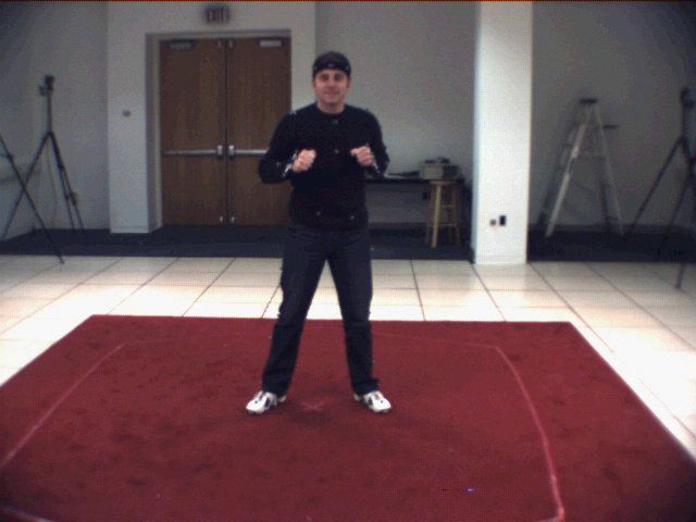
Sensors 2021, 21, 3769                                                                                          2 of 30

                         ably including the creation of new datasets. However, one step towards better in-the-wild
                         performance is discussing dataset biases and measuring cross-database performance, that
                         is training with one database and testing with another one [25]. This step was addressed in
                         our paper.
                               Our key contributions are as follows:
                         1.   We reviewed the literature (Section 2) and discussed biases in the commonly used
                              datasets Human3.6M, HumanEva-I, and Panoptic Studio (Section 3), which we also
                              used for our cross-dataset experiments;
                         2.   We proposed a method for harmonizing the dataset-specific skeleton joint definitions
                              (see Section 4.1). It facilitates cross-dataset experiments and training with multiple
                              datasets while avoiding systematic errors. The source code is available at https:
                              //github.com/mihau2/Cross-Data-Pose-Estimation (accessed on 27 May 2021);
                         3.   We proposed a scale normalization method that significantly improves generalization
                              across cameras, subjects, and databases by up to 50% (see Section 4.2). Although
                              normalization is a well-known concept, it has not been consistently used in 3D human
                              pose estimation, especially with the 3D skeletons;
                         4.   We conducted cross-dataset experiments using the method of Martinez et al. [26]
                              (Section 5), showing the negative effect of dataset biases on generalization and the
                              positive impact of the proposed scale normalization. Additional experiments investi-
                              gated the effect of using more or less cameras (including virtual cameras), training
                              with multiple datasets, applying a proposed anatomy-based pose validation step, and
                              using OpenPose as the basis for the 3D pose estimation. Finally, we discussed our
                              findings, the limitations of our work, and future directions (Section 6).

                         2. Related Work
                              Since the work of Shotton et al. [13] and the development of the Kinect sensor, enor-
                         mous research efforts have been made in the field of human pose estimation. While the
                         work at that time was often based on depth sensors, approaches developed in recent years
                         have focused primarily on estimating the human pose from RGB images. In addition to the
                         high availability of the corresponding sensors, which allows for the generation of extensive
                         datasets in the first place, this is primarily due to the development in the area of deep
                         neural networks, which are very successful in processing visual information. Therefore, all
                         current approaches are based on deep neural networks, but, according to their objectives,
                         can be roughly divided into three categories.
                              The quantitative results of prior works are summarized in Tables 1–3 for reference.

                         2.1. 2D Human Pose Estimation
                              The first class of approaches aims to predict the 2D skeleton joint positions from an
                         RGB input image. In their approach called convolutional pose machines [27], the authors
                         proposed a network architecture of cascading convolutional networks to predict belief maps
                         encoding the 2D joint positions, where each stage refines the prediction of the previous
                         stage. This approach was extended by Newell et al. [28] by replacing the basic convolutional
                         networks with repeated bottom-up, top-down processing networks with intermediate
                         supervision (stacked hourglass) to better consolidate features across all scales and preserve
                         spatial information at multiple resolutions. In [29], the pose estimation problem was split
                         into two stages. A base network with a pyramidal structure aimed to detect the 2D joint
                         positions, while a refinement network explicitly learned to predict the “hard-to-detect”
                         keypoints, i.e., keypoints that were not detected by the base network during the training
                         process. In addition to 2D keypoints, the network in the part affinity field approach [30]
                         learns to predict the orientation and location of several body parts (limbs), resulting in
                         superior keypoint detection. This is particularly helpful when it comes to associating
                         multiple detected joint positions with individuals in multi-person scenarios. This approach
                         was later integrated into the OpenPose framework [31]. In [32], the authors replaced the
                         discrete pixelwise heat map matching with a fully differentiable spatial regression loss.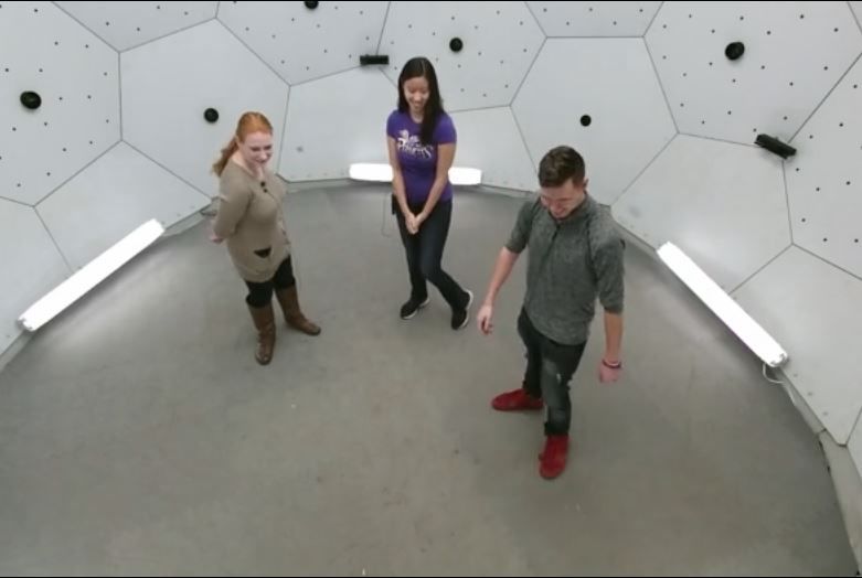
Sensors 2021, 21, 3769                                                                                                3 of 30

                         This led to an improved pose estimation, as the low resolution of the predicted heat maps
                         no longer limited the spatial precision of the detected keypoints. Furthermore, several
                         regularization strategies increasing the prediction accuracy were proposed. Human pose
                         estimation in multi-person scenarios poses a particular challenge. Top-down approaches
                         (e.g., [33]) perform a person detection (bounding boxes) followed by a single-person pose
                         estimation, but typically suffer from partial or even complete overlaps. In contrast, bottom-
                         up approaches [34] first detect all joint positions and then attempt to partition them into
                         corresponding person instances. However, this requires solving an NP-hard partitioning
                         problem. The authors in [35] addressed this problem by simultaneously modeling person
                         detection and joint partitioning as a regression process. For this purpose, the centroid of
                         the associated person was predicted for each pixel of the input image. In [36], the authors
                         first identified similarities among the several approaches for human pose estimation and
                         provided a list of best practices. In their own approach, the authors achieved a state-of-
                         the-art performance by replacing upsample layers with deconvolutional filters and adding
                         optical flow for tracking across multiple images. Whereas all other approaches obtain
                         high-resolution representations by recovering from low-resolution maps using some kind
                         of upscaling networks, Sun et al. [37] proposed HRNet, a network architecture that is able
                         to maintain high-resolution representations throughout all processing steps, leading to
                         superior performance on 2D human pose estimation.

                         Table 1. Mean per-joint position error (MPJPE) for state-of-the-art approaches on H36M.

                          Method (Reference)              MPJPE (mm)         Method (Reference)            MPJPE (mm)
                          Ionescu et al. [20]                 162.1          Habibie et al. [38]              65.7
                          Pavlakos et al. [39]                115.1          Zhou et al. [40]                 64.9
                          Chen and Ramanan [41]               114.2          Sun et al. [42]                  64.1
                          Zhou et al. [43]                    113.0          Luo et al. [44]                  61.3
                          Tome et al. [45]                     88.4          Rogez et al. [46]                61.2
                          Martinez et al. [26]                 87.3          Nibali et al. [47]               55.4
                          Pavlakos et al. [48]                 75.9          Luvizon et al. [49]              53.2
                          Wang et al. [50]                     71.9          Dabral et al. [51]               52.1
                          Tekin et al. [52]                    69.7          Li et al. [53]                   50.9
                          Chen et al. [54]                     68.0          Lin and Lee [55]                 46.6
                          Katircioglu et al. [56]              67.3          Chen et al. [57]                 44.1
                          Benzine et al. [58]                  66.4          Wu and Xiao [59]                 43.2
                          Sárándi et al. [60]                  65.7          Cheng et al. [61]                42.9

                         Table 2. Mean per-joint position error (MPJPE) for state-of-the-art approaches on the PAN dataset.

                          Method (Reference)                                                MPJPE (mm)
                          Popa et al. [62]                                                         203.4
                          Zanfir et al. [63]                                                       153.4
                          Zanfir et al. [64]                                                        72.1
                          Benzine et al. [58]                                                       68.5

                         Table 3. Mean per-joint position error (MPJPE) for state-of-the-art approaches on the HumanEva-
                         I dataset.

                          Method (Reference)                                                MPJPE (mm)
                          Radwan et al. [65]                                                       89.5
                          Wang et al. [50]                                                         71.3
                          Yasin et al. [66]                                                        38.9
                          Moreno-Noguer [67]                                                       26.9
                          Pavlakos et al. [68]                                                     25.5
                          Martinez et al. [26]                                                     24.6
                          Pavlakos et al. [39]                                                     18.3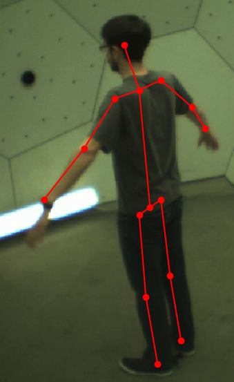
Sensors 2021, 21, 3769                                                                                           4 of 30

                         2.2. 3D Human Pose Estimation from 2D Images
                              The next class of approaches predicts 3D skeleton joint positions using raw 2D RGB
                         images as the input. Li and Chan [69] used a multitask learning approach to simultaneously
                         train a body part detector and a pose regressor using a fully connected network. In
                         contrast to the direct regression of a pose vector, Pavlakos et al. [68] transferred the idea
                         of the heat map-based 2D pose estimation into the 3D domain and predicted per-joint 3D
                         heat maps using a coarse-to-fine stacked hourglass network, where each voxel contains
                         the probability that the joint is located at this position. Each refinement stage increases
                         the resolution of the z-prediction. Tekin et al. [52] proposed fusing features extracted
                         from the raw image with features extracted from 2D heat maps to obtain a 3D pose
                         regression vector. A similar approach was developed in [40], but instead of deriving
                         features from an already predicted heat map, the authors utilized latent features from
                         the 2D pose regression network. Their end-to-end trainable approach allows for sharing
                         common representations between the 2D and the 3D pose estimation tasks, leading to
                         an improved accuracy. Dabral et al. [51] utilized the same architecture as in [40], but
                         introduced anatomically inspired loss functions, which penalize pose predictions with
                         illegal joint angles and non-symmetric limb lengths. In LCR-Net [46], the pose estimation
                         problem was split into three subtasks: localization, classification, and regression. During
                         localization, candidate boxes and a list of pose proposals are generated using a region
                         proposal network. The proposals are then scored by a classifier and subsequently refined by
                         regressing a set of per-anchor-pose vectors. The subnets share layers so that the complete
                         process can be trained end-to-end. Kanazawa et al. [70] took a slightly different approach.
                         Instead of keypoints, the authors aimed to predict a full 3D mesh by minimizing the
                         reconstruction error. Since the reconstruction loss is highly underconstrained, the authors
                         proposed an adversary training to learn whether a predicted shape is realistic or not.
                         Sun et al. [42] evaluated the performance of the differentiable soft-argmax operation as
                         an alternative to the discrete heat map loss in greater detail and verified its effectiveness.
                         Their approach achieved state-of-the-art results on Human3.6M by splitting the volumetric
                         heat maps into separate x-, y- and z-maps, which allowed for mixed training from both
                         2D and 3D datasets. Instead of directly dealing with joint coordinates, Luo et al. [44]
                         modeled limb orientations to represent 3D poses. The advantage is that orientations are
                         scale invariant and less dependent on the dataset. Their approach achieved good results on
                         several datasets and generalized well to unseen data. In [49], the authors combined action
                         recognition with human pose estimation. The proposed multitask architecture predicted
                         both local appearance features, as well as keypoint positions, which were then fused to
                         obtain the final action label. The actual pose estimation was based on heat maps and the
                         soft-argmax function. The approach showed state-of-the art results on both pose estimation
                         and action recognition. Another multitask approach was presented by Trumble et al. [71]. It
                         simultaneously estimates 3D human pose and body shape using a symmetric convolutional
                         autoencoder. However, the approach relies on multi-view camera inputs. Approaches
                         that adapt a kinematic skeleton model to the input data typically rely on the detection of
                         corresponding points. This task has been mostly addressed in scenarios where a depth
                         sensor was available. In contrast to this, DensePose [72] maps an input image to the 3D
                         surface of the human body by regressing body part-specific UV coordinates from each RGB
                         input pixel. The approach showed good results, but one has to keep in mind that identifying
                         correspondences is not yet a complete pose estimation due to possible 2D/3D ambiguities
                         and model constraints. All aforementioned approaches learned a direct mapping between
                         the input data and the pose to be estimated. This must be distinguished from approaches
                         that initially learn a latent representation of either the input or the output data [56,73].
                         In [56], an overcomplete autoencoder network was used to learn a high-dimensional latent
                         pose representation. The input image was then mapped to the latent space, leading to a
                         better modeling of the dependencies among the human joints. In contrast, Rhodin et al. [73]
                         trained a latent representation of the input data by utilizing an autoencoder structure to
                         map one camera view to another. The pose was then regressed from the latent state space.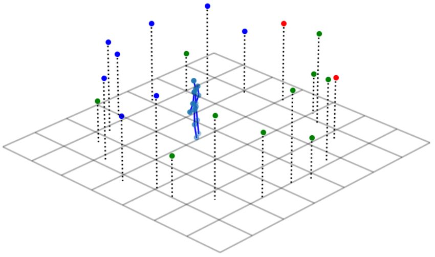
Sensors 2021, 21, 3769                                                                                         5 of 30

                         The approaches showed good, but not the best results. Sárándi et al. [60] demonstrated
                         the effectiveness of data augmentation. By occluding random positions in the RGB image
                         with samples from the Pascal VOC dataset, the mean per-joint position error (MPJPE)
                         can be reduced by up to 20%, making this approach the ECCV pose estimation challenge
                         winner in 2018. The occlusion acts as a regularizer, forcing the network to learn joint
                         positions from several visual cues. The authors used ResNet as the backbone architecture
                         to generate volumetric heat maps. As high-resolution volumetric heat maps are quite
                         memory intensive, the authors of MargiPose [47] proposed to learn three distinct heat maps
                         instead. The maps represent the xy-, xz-, and yz-plane and can be seen as projections of
                         the volumetric heat map. Their approach, which was based on the Inception v4 model,
                         achieved good results and provided a memory-efficient alternative to volumetric heat
                         maps. Habibie et al. [38] contributed by integrating 3D features in the latent space of the
                         learning process. The regressed 3D pose is back-projected to 2D before the loss is computed
                         and thus allows a 3D pose estimation based on 2D datasets. However, there is no explicit
                         supervision of the hidden feature maps that encode the 3D pose cues. A recent work by
                         Wu and Xiao [59] proposed to model the limbs explicitly. Their approach was somewhat
                         similar to OpenPose [31], but extended it to the 3D domain. Next to 2D keypoints from
                         2D heat maps, the network learned to predict densely-generated limb depth maps. Latent
                         features from the 2D pose estimator and the depth map estimation, as well as 3D specific
                         additional features were then fused to lift the 2D pose to 3D. Their approach significantly
                         outperformed all other methods on the Human3.6M and MPI-INF-3DHP datasets.

                         2.3. 3D Human Pose Estimation from the 2D Pose
                               The last class of approaches attempts to predict the 3D pose from an earlier pre-
                         dicted 2D pose, a process typically known as lifting. A big advantage of separating the
                         lifting from the 2D pose estimation is that it can be pre-trained using synthetic poses.
                         Martinez et al. [26] directly regressed 3D poses from 2D poses using only fully connected
                         layers. Their approach achieved excellent results, at least when using 2D ground truth joint
                         positions as the input. In [41], the authors built a huge library of 3D poses and matched
                         it against a detected 2D pose. Using also the stored camera parameters, the best 3D pose
                         was then scaled in a way that it matched the 2D pose. Pavllo et al. [74] exploited temporal
                         information by using dilated temporal convolutions on 2D keypoint sequences. Hossain
                         and Little [75] designed an efficient sequence-to-sequence network taking a sequence of 2D
                         keypoints as the input to predict temporally consistent 3D poses. Their approach achieved
                         state-of-the-art results for every action class of the Human3.6M dataset. While CNNs are
                         suitable for processing grid-like input data (e.g., images), graph convolutional networks
                         (GCNs) can be seen as a generalization of CNNs acting on graphs. In [76], Zhao et al.
                         exploited the hierarchical structure of skeletons by describing both 2D and 3D skeletons as
                         graphs and used CGNs to obtain 3D poses from 2D poses. The aforementioned approaches
                         reported excellent results, in particular when temporal information was used. However,
                         they heavily relied on the quality of the underlying 2D pose estimator. If no 2D ground
                         truth was used, the accuracy was typically similar to approaches that obtained 2D and 3D
                         poses directly from the image.

                         2.4. Cross-Dataset Generalization
                              Comprehensive datasets are required in order to train methods for pose estimation.
                         In contrast to 2D pose estimation, reliable 3D pose data cannot be obtained by manually
                         annotating images taken in-the-wild, but are acquired with the help of motion capture
                         systems (e.g., VICON [77], The Captury [78], IMU). This typically limits the acquisition to
                         controlled in-the-lab environments with low variations in terms of subjects, camera view
                         points, backgrounds, occlusions, lighting conditions, etc. This raises the questions how
                         well these approaches (a) perform across multiple controlled datasets and (b) generalize to
                         unconstrained in-the-wild data. Work in this area is still limited. The typical approach is
                         to combine in-the-wild 2D pose data with in-the-lab 3D pose data. Mehta et al. [23] used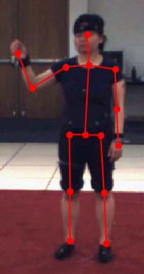
Sensors 2021, 21, 3769                                                                                            6 of 30

                         transfer learning to transfer knowledge from a pre-trained 2D pose network to a 3D pose
                         regression network [23]. They further provided the MPI-INF-3DHP dataset, an augmented
                         in-the-wild 3D pose dataset, by utilizing a marker-less multi-camera system [78] and
                         chroma keying (green screen). The best results on Human3.6M were achieved using
                         transfer learning and including additional data from MPI-INF-3DHP. Zhou et al. [40]
                         mixed 2D and 3D data per batch to learn common representations between 2D and 3D
                         data by computing additional depth regression and anatomical losses for 3D training
                         samples [40]. When additional 2D pose data from the MPII dataset were included, errors
                         on the Human3.6M dataset were reduced by up to 15 mm, and the proportion of correctly
                         estimated joints (PCKs) increased from 37.7% to 69.2% on the MPI-INF-3DHP dataset.
                         This indicated that the constrained setting of Human3.6M is insufficient to generalize
                         to in-the-wild data. The authors also concluded that adding additional 2D data did not
                         improve the accuracy of the 2D pose prediction, but mostly benefited the depth regression
                         via shared feature representations. As mentioned above, Habibie et al. [38] circumvented
                         the problem of missing 3D pose labels by learning both view parameters and 3D poses. The
                         3D poses were then back-projected to 2D (using a trainable network) before applying the
                         2D loss. Their approach showed high accuracy and generalized well to in-the-wild scenes.
                         Other approaches attempt to generate 3D labels from existing 2D datasets. Wang et al. [79]
                         achieved this by first mapping a 2D pose to 3D using a “stereo-inspired” neural network
                         and then refined the 3D pose using a geometric searching scheme so that the determined
                         3D pose matched the 2D pose with pixel accuracy. In [80], which was an updated version
                         of [46], Rogez et al. [46] created pseudo 3D labels for 2D datasets by looking for the 3D
                         pose that best matched a given 2D pose in a large-scale 3D pose database. Further work
                         addressed the problem of missing 3D pose labels by generating synthetic datasets by
                         animating 3D models [81,82] or rendering textured body scans [83]. While rendering may
                         seem promising, both integrating human models in existing images, as well as rendering
                         realistic scenes are not trivial and often require a domain adaption to generalize from
                         synthetic to real images [81,83,84]. Therefore, Rogez and Schmid [85] proposed to build
                         mosaic pictures of real images from 2D pose datasets. While artificial looking, the authors
                         showed that CNNs can be trained on these image and generalize well to real data without
                         the need for any fine-tuning and domain adaption.
                              While many authors combined multiple training datasets, work on cross-dataset eval-
                         uation is still limited. To the best of our knowledge, the very recent work of Wang et al. [86]
                         was the first to systematically examine the differences among existing pose datasets and
                         their effect on cross-database evaluation. However, they focused on systematic differ-
                         ences of camera viewpoints and conducted their experiment with another set of databases,
                         compared to our work.

                         2.5. Non-Vision-Based Approaches
                              All approaches listed so far were based on optical sensors, i.e., cameras. We would like
                         to point out to the reader that besides visual methods, other ranges of the electromagnetic
                         spectrum can also be used to estimate the human pose. The major advantage of these
                         approaches is that they are independent of lighting, background, as well as clothing and
                         even allow for person detection and pose estimation through walls and foreground objects.
                         Moreover, privacy issues can be avoided in contrast to camera-based approaches. The most
                         prominent examples are microwaves and millimeter waves. In [16], the authors proposed
                         a radar-based approach (operating in the 5.56–7.25 GHz range) for indoor person location,
                         obtaining a spatial resolution of 8.8 cm. In RFPose [17], the authors utilized radio frequency
                         (RF) signals (20 kHz–300 GHz) and visual information to extract 2D skeleton positions.
                         The approach was later extended to 3D [87], where the authors reported a mean per-joint
                         localization error of 4.2 cm, 4.0 cm, and 4.9 cm for the X-, Y-, and Z-axes, respectively.
                         However, a major disadvantage of this approach is the very specific and high hardware
                         requirements (synchronized 16 + 4 T-shaped antenna array with frequency-modulated
                         continuous waves), which severely limit its possible applications. There are also LIDAR-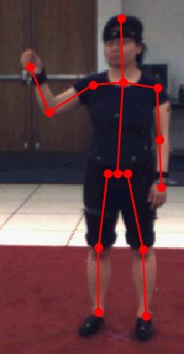
Sensors 2021, 21, 3769                                                                                            7 of 30

                         based approaches (e.g., [18]), but these are usually expensive and power consuming. More
                         recently, WiFi-based approaches were proposed. In [88], Wang et al. [88] developed a
                         human pose estimation system, which reconstructed 2D skeletons from WiFi by mapping
                         the WiFi data to 2D joint heat maps, part affinity fields, and person segmentation masks.
                         The authors reported an average percentage of correctly detected keypoints (PCK) of 78.75%
                         (89.48% for OpenPose [31]). However, their approach performed significantly worse in
                         untrained environments (mPCK = 31.06%). This is a main challenge for all WiFi-based
                         approaches, as WiFi signals exhibit significantly different propagation patterns in different
                         environments. To address this issue and achieve cross-environment generalization, the
                         authors of WiPose [89] proposed to utilize 3D velocity profiles obtained from WiFi signals
                         in order to separate posture-specific features from the static background objects. Their
                         approach achieved an accuracy of up to 2.83 cm (mean per-joint position error), but is
                         currently limited to a single non-moving person.
                               Camera-based approaches are passive methods, as they capture the ambient light
                         reflected by an object. In contrast, RF-based methods can be considered as active methods,
                         since an illumination signal is actively emitted and interacts with the objects in the scene
                         before being reflected and measured by the receiver. Here, the active illumination signal
                         is often based on appropriately modulated waves or utilizes stochastic patterns. A major
                         drawback of this approach is that the active signal is not necessarily ideal for the specific
                         task, i.e., it is not possible to distinguish between relevant and irrelevant information
                         during the measurement process.
                               This leads to the idea of learned sensing [90], in which the measurement process
                         and the processing of the measurement data are optimized in an overall system. This
                         requires the availability of programmable transmitter hardware whose configuration is
                         determined using machine learning methods in such a way that the emitted illumination
                         signal is optimal for the respective measurement process. This approach has recently been
                         successfully implemented for person recognition, gesture recognition, and human pose
                         estimation tasks. See [91,92] for further details. The idea of learned sensing was also applied
                         in the optical domain in order to determine optimal illumination patterns for specific
                         microscopy tasks [93].
                               For human pose estimation, the learned sensing approach cannot easily be transposed
                         to optical sensors. This is mainly due to the fact that changes in the active illumination
                         signal can be perceived by humans, which is typically undesirable in real-world scenar-
                         ios. Nevertheless, we suspect that the method can be transferred to approaches that use
                         special (infrared) photodiodes to determine the pose [94]. Furthermore, there may be
                         an application opportunity in multi-camera scenarios. These are often associated with a
                         costly measurement process (high energy consumption, data volume, latency), whereas
                         only a specific part of the measured data is actually required to resolve potentially occur-
                         ring ambiguities.

                         3. Datasets
                              In the following subsections, we describe the three 3D human pose estimation datasets
                         that we used in this article: HumanEva-I, Human 3.6M, and Panoptic. Afterwards, we
                         compare the datasets and discuss dataset biases.

                         3.1. HumanEva-I (HE1)
                              In 2006 and 2010, Sigal et al. [21,22] published the HumanEva-I and HumanEva-
                         II datasets to facilitate the quantitative evaluation and comparison of 3D human pose
                         estimation algorithms. We used HumanEva-I, which is larger and more diverse than
                         HumanEva-II. In HumanEva-I, each of four subjects performs six actions (walking, jogging,
                         gesturing, throwing/catching a ball, boxing, and a sequence of several actions) while being
                         recorded with seven cameras. The ground truth positions of the 15 provided skeleton joints
                         were obtained with a motion capture system using reflective markers.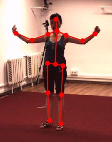
Sensors 2021, 21, 3769 8 of 30
3.2. Human3.6M (H36M)
Ionescu et al. [19,20] collected and published Human3.6M, which is comprised of
3.6 million frames showing diverse body poses of actors performing 15 everyday actions
including conversations, eating, greeting, talking on the phone, posing, sitting, smoking,
taking photos, waiting, and walking. It total, eleven actors were involved, but they
performed individually one after another (i.e., only one person was visible in each video).
The data were recorded with four color video cameras and a marker-based motion capture
system, providing thirty-two skeleton joint positions.
3.3. Panoptic (Pan)
Aiming at analyzing social interaction, Joo et al. [10,11] recorded the Panoptic Stu-
dio dataset. In its current state (Version 1.2), it is comprised of 84 sequences with more
than 100 subjects. The sequences are very diverse, among others covering: social games
(Haggling, Mafia, and Ultimatum) with up to eight subjects; playing instruments; dancing;
playing with toddlers; and covering range of motion. In contrast to the other datasets, there
is no categorization or segmentation of the actions (beyond the above-mentioned categories
of sequences). To record the dataset, Joo and colleagues built the Panoptic Studio, a special
dome with more than 500 cameras in its walls. Using these cameras, Joo et al. [10,11]
developed an algorithm for obtaining multi-person 3D skeleton joint ground truths with-
out markers. Their algorithm was based on 2D body pose estimation providing “weak”
proposals, triangulation and fusion of the proposals, and temporal refinement.
3.4. Comparison and Dataset Biases
Computer vision datasets are created for quantitatively measuring and comparing
the performance of algorithms. However, “are the datasets measuring the right thing, that
is, the expected performance on some real-world task?,” Torralba and Efros asked in their
article on dataset biases [25]. We were interested in the task of relative 3D human body
pose estimation in the real world, not only in a specific laboratory. Therefore, we may
ask if the error in estimating poses on a specific dataset resembles the expected error in
real-world application. Are these datasets representative samples of real-world data or are
they biased in some way?
Currently, most “in-the-wild” datasets are collected from the Internet, including
datasets commonly used for 2D human body pose estimation [95,96]. Although these
datasets are very diverse, they may still suffer from biases compared to the real world, e.g.,
capture bias (pictures/videos are often taken in similar ways) or selection bias (certain
types of images are uploaded or selected for datasets more often) [25].
The datasets of 3D pose estimation are less diverse. They are typically recorded in
a laboratory, because (1) multi-view camera systems are state-of-the-art for measuring
accurate 3D ground truths and (2) building, installing, and calibrating these systems
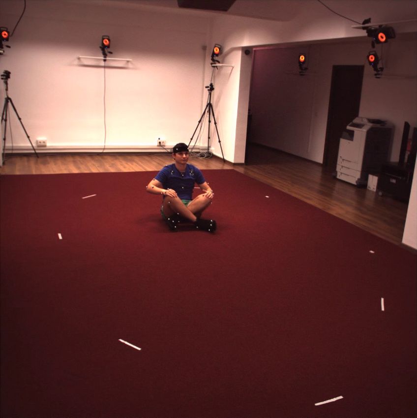
requires much effort (making it hard to move the systems). All three datasets, HumanEva-
I, Human3.6M, and Panoptic, were recorded in such an indoor laboratory with very
controlled conditions; see Figure 1 for some example images. The datasets differ in size
and diversity, as summarized in Table 4. Compared to in-the-wild data, the three datasets
suffer from several biases:
• Lighting: The recordings are homogeneously lit, typically without any overexposed
or strongly shadowed areas. Further, there is no variation in lighting color and color
temperature. Real-world data are often more challenging, e.g., consider an outdoor
scene with unilateral sunlight or a nightclub scene with colored and moving lighting;
• Background: The backgrounds are static and homogeneous. Real-world data often
include cluttered and changing backgrounds, which may challenge the computer
vision algorithms more;
• Occlusion: In real-world data, people are often partially occluded by their own body
parts, other people, furniture, or other objects; or parts of the body are outside the
image. Self-occlusion is covered in all three databases. Human3.6M is comprised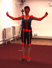
Sensors 2021, 21, 3769                                                                                                      9 of 30

                                      of more self-occlusions than the other datasets (and also some occlusions by chairs),
                                      because it includes many occlusion-causing actions such as sitting, lying down, or
                                      bending down. Occlusions by other people are common in Panoptic’s multi-person
                                      sequences. Additionally, parts of the bodies are quite frequently outside of the cameras’
                                      field of view in Panoptic;
                                 •    Subject appearance: Human3.6M and especially HumanEva-I suffer from a low num-
                                      ber of subjects, which restricts variability in body shapes, clothing, hair, age, ethnicity,
                                      skin color, etc. Although Panoptic includes many more and quite diverse subjects, it
                                      may still not sufficiently cover the huge diversity of real-world human appearances;
                                 •    Cameras: In-the-wild data are recorded from different viewpoints with varying res-
                                      olutions, noise, motion blur, fields of view, depths of field, white-balance, camera-
                                      to-subject distance, etc. Within the three databases, only the viewpoint is varied
                                      systematically, and the other factors are mostly constant. With more than 500 cameras,
                                      Panoptic is the most diverse regarding viewpoint (also using three types of cameras).
                                      In contrast to the others, it also includes high-angle and low-angle views (down-
                                      and up-looking cameras). If only a few cameras are used, as in Human3.6M and
                                      HumanEva-I, there may be a bias in the body poses, because people tend to turn
                                      towards one of the cameras (also see [86] on this issue);
                                 •    Actions and poses: HumanEva-I and Human3.6M are comprised of the acted behavior
                                      of several action categories, whereas the instructions in Human3.6M allowed quite
                                      free interpretation and performance. Further, the actions and poses in Human3.6M
                                      are much more diverse than in HumanEva-I, including many everyday activities and
                                      non-upright poses such as sitting, lying down, or bending down (compared to only
                                      upright poses in HumanEva-I). However, some of the acted behavior in Human3.6M
                                      used imaginary objects and interaction partners, which may cause subtle behavioral
                                      biases compared to natural interaction. Panoptic captured natural behavior in real
                                      social interactions of multiple people and interactions with real objects such as musical
                                      instruments. Thus, it should more closely resemble real-world behavior;
                                 •    Annotated skeleton joints: The labels of the datasets, the ground truth joints provided,
                                      differ among the datasets in their number and meaning. Most obviously, the head,
                                      neck, and hip joints were defined differently by the dataset creators. In Section 4.1,
                                      we discuss this issue in detail and propose a way to handle it.

          Figure 1. Example images of the HumanEva-I (left), the Human3.6M (middle), and the Panoptic databases (right).

                                 Table 4. Quantitative comparison of the datasets.

                                                               HumanEva-I             Human3.6M                  Panoptic
                                  Subjects                           4                      11                    >100
                                  Actions                            6                      15                    many
                                  Multi-person                       -                       -                      X
                                  Recording duration              10 min                 298 min                 689 min
                                  Cameras                            7                       4                    >500
                                  Total frames                    0.26 M                  3.6 M                  >500 M
                                  Skeleton joints                   15                      32                      19
Sensors 2021, 21, 3769 10 of 30
Although all the datasets have been and still are very useful to advance the state-of-
the-art, we expect that many of these datasets’ biases will degrade real-world performance
in 3D human pose estimation. As all the datasets were sampled from the real world, we
used training and testing with different databases as a surrogate for roughly estimating the
expected in-the-wild performance. Such cross-database evaluation is a common practice or
a targeted goal in many other domains of computer vision [25,97–102].
Some of the biases, such as lighting, background, as well as subject ethnicity, clothing,
and hair, only affect the images, but not the position of body joints. A limited diversity in
these factors may be acceptable in 3D pose estimation datasets, because it is no problem for
training a geometry-based approach that estimates the 3D pose from the 2D joint positions,
given the used 2D pose estimation model has been trained with a sufficiently diverse 2D
pose estimation dataset. Other factors, especially cameras and poses, heavily influence
the position of body joints and must be covered in great diversity in both 2D and 3D
pose datasets.
4. Methods
4.1. Joint Harmonization
As mentioned before, the skeleton joint positions provided in the datasets differed in
their number and definition. To be able to conduct cross-dataset experiments, we selected
a common set of 15 joints based on HumanEva-I. One keypoint was the central hip joint,
which is the origin of the local body coordinate system, i.e., it is always at (0, 0, 0). Thus,
we excluded it from the training and error evaluation. The remaining 14 joints are listed
in Table 5. The first problem we faced was that there was no head keypoint in Panoptic,
because this has not been annotated in the MS COCO dataset [96], which is used for training
OpenPose [27,31] and other 2D pose estimators. However, there are MS COCO keypoints
for the left and right ear. We calculated the center of gravity of these two points (Number
17 and 18 in Panoptic and OpenPose) in order to get a keypoint at the center of the head.
Table 5. Our joint definitions for the different datasets and OpenPose. The numbers in the table
correspond to the joint number in the datasets’ original joint definition. The joints marked with *
were repositioned in the harmonization process.
Joint HumanEva-I Human3.6M Panoptic OpenPose
R Hip 1* 1* 12 9
R Knee 2 2 13 10
R Ankle 3 3 14 11
L Hip 4* 6* 6 12
L Knee 5 7 7 13
L Ankle 6 8 8 14
Neck 7 13 * 0 1
Head 8* 15 * (17 + 18)/2 (17 + 18)/2
L Shoulder 9 17 3 5
L Elbow 10 18 4 6
L Hand 11 19 5 7
R Shoulder 12 25 9 2
R Elbow 13 26 10 3
R Hand 14 27 11 4
After this step, we had keypoints for all the joints listed in Table 5. However, there
were still obvious differences in some of the joints’ relative placements, as illustrated in
Figure 2a,c,e. The different skeleton joint definitions introduced systematic errors into the
cross-dataset experiments. To counter these effects, we harmonized the joint positions,
using Panoptic (and thus the MS COCO-based joints) as the reference. This facilitated
combining the 3D pose estimation with MS COCO-based 2D pose estimators, which is a
promising research direction, and comparing future results with ours.Sensors 2021, 21, 3769 11 of 30
(a) orig. joints, HE1 (b) harm. joints, HE1 (c) orig. joints, H36M (d) harm. joints, H36M (e) orig. joints, PAN
Figure 2. Examples showing the skeleton of HumanEva-I (HE1) and Human3.6M (H36M) before (“original” = orig.) and after
the harmonization (harm.) of the head, neck, and hip joints. Panoptic (PAN) was used as the reference for harmonization.
We adjusted the obvious differences in the head, neck, and hip positions in the
HumanEva-I (HE1) and Human3.6M (H36M) datasets: (1) the head joint was moved to in
between the ears in both HE1 and H36M; (2) the neck was placed between the shoulders in
the H36M; and (3) the hip width (distance between the left and right hip keypoints) was
expanded in HE1 and reduced in H36M.
To be more precise, the positions of the head and hip joints of the HE1 dataset were
harmonized as follows: To move the head closer to the neck, we multiplied the direction
vector between the neck and the head joint by a factor of 0.636. We calculated the factor
from the ratio of the means of the neck-to-head length of the HE1 (316.1 mm) and the
Panoptic (PAN) test datasets (201.1 mm). The hip joint distance was increased from the
common center point by a factor of 2.13, again based on scaling the direction vector by the
ratio of the mean distances (PAN 205.2 mm, HE1 96.3 mm). Figure 2a,b illustrates the effect
of our adjustment.
The joint harmonization of the H36M dataset changed the position of the neck, head,
and hip joints. The neck joint, which was defined at a higher position than in the other
datasets, was moved to the center between the shoulder joints. To move the head point
closer to the neck, we multiplied the direction vector between the repositioned neck joint
and the head joint by a factor of 0.885. The factor was calculated from the ratio of the
means of the neck-to-head length of the H36M (227.3 mm) and the PAN test datasets
(201.1 mm). The hip joint distance was reduced from the common center point to 0.775
of the original value, based on the mean distances (PAN 205.2 mm, H36M 264.9 mm).
Figure 2c,d illustrates the effect of the adjustment.
We provided the Python source code for harmonizing the joints at https://github.
com/mihau2/Cross-Data-Pose-Estimation/ (accessed on 27 May 2021).
4.2. Scale Normalization
People differ in their heights and limb lengths. On the one hand, this is a problem for
2D-image-based 3D pose estimation, because, in the general case, the real height and limb
lengths of a person (as well as the distance from the camera) cannot be measured from a
single 2D image; therefore, accurate estimation of 3D joint positions is only possible up to
an unknown scaling factor. Nevertheless, most state-of-the-art methods train their relative
pose estimation models in a way that forces them to implicitly predict this scale, because
they train the models to predict 3D joint coordinates, which implicitly contain the overall
scale and the body proportions. This imposes a burden that encourages the models to learn
dataset-specific heuristics, such as the height of individual subjects, the mean height of the
subjects, the characteristics of the camera used, or the expected height/depth depending
on the position and/or size of the person in the image. We expect that this way of training
worsens generalization to in-the-wild data and in cross-dataset evaluations. On the otherSensors 2021, 21, 3769 12 of 30
hand, knowing the scaling factor (the real height and limb lengths of the person) is not
necessary for many applications that only require relative joint positions. Normalizing the
joint positions from absolute to relative coordinates is common practice. We went a step
further and proposed to normalize the scale of the skeletons, in order to remove the (often
unnecessary) burden of predicting the scale and to improve the cross-dataset performance.
The absolute joint coordinates pi of each pose sample were normalized individually
based on the skeleton’s relative joint positions in relation to the center hip point p0 , which
was in the origin of the local coordinate system. We quantified the scale s by calculating
the mean of the Euclidean distances between the origin and all N joint positions:
N
1
s=
N ∑ k p i − p0 k (1)
i =1
Afterwards, we resized the skeleton by dividing all joint position coordinates by the
scale, yielding a normalized scale of 1. The normalized joint positions p̂i were calculated
as follows:
1
p̂i = (pi − p0 ) (2)
s
This normalized all poses to a similar coordinate scale. This transformation was
applied individually in both the 3D target data (with pi ∈ R3 ) and the 2D input data (with
pi ∈ R2 ).
4.3. Baseline Model and Training
We performed our experiments with the “Baseline” neural network architecture
proposed by Martinez et al. [26]. We decided to use an existing method rather than
developing a completely new approach, because the focus of our work was on cross-
dataset evaluation and proposing improvements that can be applied in many contexts. The
approach by Martinez et al. did not rely on images, but mapped 2D skeleton joint positions
to relative 3D joint positions, which is also called “lifting”. Thus, it can be combined with
any existing or future 2D body pose estimation method. This way, the results can benefit
from advances in 2D pose estimation, which are faster than in 3D pose estimation, because
in-the-wild 2D pose datasets are much easier to create than their counterparts with 3D
ground truths. Other advantages include: (1) The approach is independent of image-related
issues, such as lighting, background, and several aspects of subject appearance, which are
covered with great diversity in 2D pose datasets. By decoupling the 2D pose estimation
from the “lifting”, we avoided overfitting the 3D pose estimation to the quite restricted
diversity of the 3D pose datasets regarding lighting, background, and subject appearance.
(2) The approach allowed augmenting the training data by creating synthetic poses and
virtual cameras, which can massively increase the variability of the available data and
lead to better generalization. (3) No images were needed, so additional sources of training
data may be exploited, such as motion capture data recorded in sports, biomechanics, or
entertainment. (4) The source code is available. Therefore, it is easy to reproduce the results,
apply the method with other data, and start advancing the approach.
The architecture by Martinez et al. [26] was a deep neural network consisting of fully
connected layers and using batch normalization, ReLU, dropout, and residual connections.
The first layer maps the 2D coordinates (2n = 28 dimensions) to a 1024-dimensional
space. It is followed by two residual blocks, each including two fully connected layers.
Finally, there is another linear layer that maps the 1024-dimensional space to the 3n = 42-
dimensional 3D coordinate output.
The model, training, and testing were implemented in the TensorFlow2 deep learning
framework using the Keras API. The networks were trained with the Adam optimizer,
minimizing the mean squared error loss function. The training set was separated into
training and validation data with a 90/10% split, and the training data were shuffled before
each epoch. We used a batch size of 512 and a dropout rate of 0.5. The training of each
neural network started with a learning rate of 10−3 , which was reduced during the trainingSensors 2021, 21, 3769 13 of 30
by a factor of 0.5 if the loss on the validation set did not decrease for 3 epochs. The training
was stopped if the validation loss did not decrease for 10 epochs or the learning rate was
reduced below 10−6 . The model with the lowest validation loss was saved for testing.
4.4. Anatomical Pose Validation
We proposed an optional pose validation step, which assessed the predicted poses
using the constraints of human anatomy. The human body is usually symmetrical regard-
ing the length of the left and right extremities and has, according to Pietak et al. [103],
stable ratios regarding the lengths of the upper and lower limbs with little variation
between individuals.
For every pose, the ratios of each upper and lower extremity, as well as its left and
right counterpart were calculated. The ratios were measured as the difference in length in
%, based on the shorter of the two compared limbs. Therefore, a ratio of 2:1 and 1:2 would
both result in a difference of +100%. If one of the 8 calculated ratios was greater than 100%,
the pose was rejected by the validation.
The effect of this approach is analyzed in Section 5.7. All the other experiments were
conducted without applying this validation step, because it led to the exclusion of rejected
poses from the error calculation and thus limited the comparability of the error measures
(which may be based on different subsets of the data).
4.5. Use of Datasets
Each dataset was split into training and test data based on the sessions/subjects and
cameras, as illustrated in Figure 3. No single camera or session was used for both the
test and training set. Although parts of the datasets were unused, we selected this way
of splitting because our focus was to measure the generalization across subjects, camera
viewpoints, and datasets rather than reaching the highest in-dataset performance. The
cameras were assigned to the test set and the reduced and full training set, as illustrated
in Figure 4 and detailed below. Further, because the number of cameras was quite low in
Human3.6M (only 4), we generated synthetic camera views as described in Section 4.5.2.
After the main split, the training data was further randomly split into 90%, which were used
as the actual training set by the optimizer, and 10%, which were used as the validation set.
Figure 3. Separation of the training and test sets for the subject sessions and camera sets (blue:
reduced training camera set; blue and green: full training camera set; red: test camera set; white:
unused data).Sensors 2021, 21, 3769 14 of 30
(a) HE1 (b) H36M (c) PAN
Figure 4. Camera positions and an example pose for the used datasets (grid at z = 0 with 1 meter cell size; blue: reduced
training camera set; blue and green: full training camera set; red: test camera set).
4.5.1. Dataset Split Details
For HumanEva-I (HE1), Subjects 0 and 1 were used as the training set and Subject 2 as
the test set. The camera “BW1” was used for the test set. We used the other black-and-white
and color cameras for the training set. The reduced camera set only contained the black-
and-white cameras. For the evaluation using the OpenPose 2D joint positions, we used all
videos of Subject 2 that contained the corresponding video and motion capture data. This
reduced the OpenPose test dataset, in comparison to the standard test set, because only a
subset of the sessions included both motion capture and video files.
For Human3.6M (H36M), Subjects 1, 5, 6, 7, and 8 were used for the training set and
Subjects 9 and 11 for testing. We used Camera 3 as the test camera. Cameras 0, 1, and 2
were the reduced camera training set. The full camera training set contained Cameras 0, 1,
and 2 and their modified synthetic copies (see Section 4.5.2). For the evaluation using the
generated OpenPose 2D joint estimations, we used all videos of Subjects 9 and 11.
For Panoptic (PAN), the Range of Motions sessions (sequence names: 171026_pose1,
171026_pose2, 171026_pose3, 171204_pose1, 171204_pose2, 171204_pose3, 171204_pose4,
171204_pose5, 171204_pose6) were used for testing and all other sessions for training. Of
each panel, we only used VGA Camera No. 1. The cameras on Panels 9 and 10 were used
for testing. The cameras on Panels 1–8 were the reduced camera training set, and the
cameras on Panels 1–8 and 11–20 were the full training set.
Table 6 shows the resulting sample sizes for the different databases and successfully
mapped OpenPose (OP) samples.
Table 6. Sample sizes in thousands of poses.
Training Set Testing Set
Reduced Full
HE1 113 225 17.8
H36M 1169 2312 137.7
PAN 4131 9809 292.0
HE1 (OP) - - 1.7
H36M (OP) - - 52.1
4.5.2. Virtual Camera Augmentation
The H36M dataset was recorded with only 4 cameras. In order to make the ratio of
training and test cameras in the databases more similar, three more camera were added.
For this purpose, we virtually copied the training Cameras 0, 1, and 2 by rotating their
extrinsic camera parameters by 90◦ around the world coordinate center in the middle of
the recording space without changing the intrinsic camera parameters. This can be seen in
Figure 4b, where the blue points represent the original training camera positions, and the
newly created cameras are shown in green.Sensors 2021, 21, 3769 15 of 30
4.6. Implementation Details
First, the original 3D pose data in the world coordinate space were loaded. If a pose
contained a non-valid joint position, usually (0, 0, 0), the pose was discarded. Further, we
used the jointwise confidence score provided in the PAN dataset to remove unreliable data.
If the score of any of the 14 used joints wasSensors 2021, 21, 3769 16 of 30
The prediction speed on the trained models was tested using an NVIDIA GeForce
RTX 2080 TI graphics card. A batch with a size of 256 samples was calculated in around
30 milliseconds, which would result in 8533 pose estimations per second. The proposed
model can therefore calculate 3D poses from 2D points in real time.
5.1. Joint Harmonization
Table 7 shows the mean and standard deviation of the errors for the evaluation over
all datasets with and without joint harmonization. All entries in a row share the same
training database; those in a column share the same test database. On the main diagonal
are the in-database errors, which were significantly lower than the cross-database error
(off the main diagonal). This difference showed the presence of dataset biases and their
negative effect on cross-dataset generalization
The joint harmonization improved the results significantly from an overall mean
error of 133.7 mm to 120.0 mm (p = 0.040, paired t-test). The impact differed among the
individual training and test dataset combinations. As to be expected, the estimation error
was mainly reduced in the cross-database results, where it was decreased by up to −29%.
The greatest effect can be seen for HE1, which was the smallest dataset and whose joint
definition deviated most from those of the other datasets.
The high absolute errors of the models trained with the HE1 were especially prominent
in the ankle and knee joints. The errors can be attributed to the low diversity of poses
in HE1, which did not include wide arm movements and no non-standing poses, which
however were very common in H36M and PAN.
Table 7. Errors with original vs. harmonized joints (no-alignment errors in mm, mean ± std. deviation).
Training Data Test Data
HE1 H36M PAN
original joints (mean 133.7)
HE1 95.9 ± 2.9 299.7 ± 9.5 148.8 ± 4.9
H36M 142.1 ± 3.9 67.6 ± 0.6 95.1 ± 3.2
PAN 166.7 ± 2.4 143.6 ± 1.2 43.9 ± 0.3
harmonized joints (mean 120.0)
HE1 91.7 ± 1.9 254.1 ± 5.8 125.4 ± 4.3
H36M 141.7 ± 3.8 67.0 ± 0.6 98.3 ± 2.2
PAN 117.8 ± 2.4 140.4 ± 1.3 43.7 ± 0.2
mean error change
HE1 −4.3% −15.2% −15.7%
H36M −0.2% −0.9% 3.4%
PAN −29.3% −2.3% −0.6%
One-sided paired-sample t-test p = 0.040.
5.2. Number of Cameras
We compared the estimation error for the full camera set with a reduced camera set.
For this purpose, the amount of used cameras was halved. Details about the used camera
sets and their placement can be found in Section 4.5 and Figure 4.
Table 8 shows the results. The use of more cameras, and therefore more viewpoints
and pose samples, changed the individual testing errors by in between 6.8% and −28.8%.
Overall, the mean error decreased from 132.6 mm to 120.0 mm, which was a statistically
significant difference (p = 0.031 in a one-sided paired t-test). The increase in the number of
cameras had a positive impact on the testing results when training with the HE1 or H36M
dataset, which both only had three camera views in the reduced camera set, with changes
in the error of −5.1% up to −28.8%.Sensors 2021, 21, 3769 17 of 30
Table 8. Errors with the reduced vs. the full camera set (no-alignment errors in mm, mean ± std.
deviation).
Training Data Test Data
HE1 H36M PAN
reduced camera set (mean 132.6)
HE1 96.6 ± 1.9 270.6 ± 11.5 176.2 ± 5.4
H36M 166.4 ± 7.7 75.1 ± 0.4 105.2 ± 5.5
PAN 129.5 ± 2.1 131.4 ± 0.7 42.2 ± 0.3
full camera set (mean 120.0)
HE1 91.7 ± 1.9 254.1 ± 5.8 125.4 ± 4.3
H36M 141.7 ± 3.8 67.0 ± 0.6 98.3 ± 2.2
PAN 117.8 ± 2.4 140.4 ± 1.3 43.7 ± 0.2
mean error change
HE1 −5.1% −6.1% −28.8%
H36M −14.8% −10.7% −6.6%
PAN −9.0% 6.8% 3.4%
One-sided paired-sample t-test p = 0.031.
5.3. Scale Normalization
Table 9 shows the mean error and the standard deviation for the evaluation with
and without scale normalization. Scale normalization significantly decreased the pose
estimation error, from on average 120.0 mm to 90.1 mm (p = 0.015 in a one-sided sample-
paired t-test). For the in-database evaluation, the error decreased between −13.2% and
−24.6%. Cross-database testing resulted in even bigger reductions up to −42.9%.
The results of the models trained on HE1 and H36M and tested on the PAN dataset
showed less improvement or even a worse result when using scale normalization. This
error increase can be attributed to the test samples with a low camera viewing angle, which
was not contained in the HE1 and H36M datasets.
Table 9. Error with and without scale normalization (no-alignment errors in mm, mean ± std.
deviation).
Training Data Test Data
HE1 H36M PAN
no scale normalization (mean 120.0)
HE1 91.7 ± 1.9 254.1 ± 5.8 125.4 ± 4.3
H36M 141.7 ± 3.8 67.0 ± 0.6 98.3 ± 2.2
PAN 117.8 ± 2.4 140.4 ± 1.3 43.7 ± 0.2
with scale normalization (mean 90.1)
HE1 69.2 ± 0.7 170.3 ± 4.0 152.7 ± 2.7
H36M 86.0 ± 1.2 55.2 ± 0.5 89.2 ± 0.7
PAN 67.3 ± 1.0 83.1 ± 0.6 37.9 ± 0.4
mean error change
HE1 −24.6% −33.0% 21.8%
H36M −39.3% −17.7% −9.3%
PAN −42.9% −40.8% −13.2%
One-sided paired-sample t-test p = 0.015.
Interestingly, the scale normalization error when training on PAN and testing on HE1
decreased below the in-database error of HE1. The training set of PAN was larger and
more diverse than that of HE1, which helped the cross-dataset generalization outperform
the in-dataset generalization in this case.
Figure 5 shows the jointwise errors with and without scale normalization of only the
cross-database evaluation as a box plot. The median error decreased for all joints, most for
the leg joints. Most of the high-error outliers occurring with the original representation
disappeared when using scale normalization.You can also read