Spatial distribution analysis of the OMI aerosol layer height: a pixel-by-pixel comparison to CALIOP observations
←
→
Page content transcription
If your browser does not render page correctly, please read the page content below
Atmos. Meas. Tech., 11, 2257–2277, 2018
https://doi.org/10.5194/amt-11-2257-2018
© Author(s) 2018. This work is distributed under
the Creative Commons Attribution 4.0 License.

Spatial distribution analysis of the OMI aerosol layer height:
a pixel-by-pixel comparison to CALIOP observations
Julien Chimot1,a , J. Pepijn Veefkind1,2 , Tim Vlemmix2 , and Pieternel F. Levelt1,2
1 Department  of Geoscience and Remote Sensing (GRS), Civil Engineering and Geosciences, TU Delft, the Netherlands
2 Royal Netherlands Meteorological Institute, De Bilt, the Netherlands
a now at: European Organisation for the Exploitation of Meteorological Satellites (EUMETSAT), Darmstadt, Germany

Correspondence: Julien Chimot (julien.chimot@eumetsat.int)

Received: 26 October 2017 – Discussion started: 7 November 2017
Revised: 17 March 2018 – Accepted: 22 March 2018 – Published: 19 April 2018

Abstract. A global picture of atmospheric aerosol vertical        1   Introduction
distribution with a high temporal resolution is of key impor-
tance not only for climate, cloud formation, and air quality      Aerosols are small particles suspended in the air (e.g. desert
research studies but also for correcting scattered radiation      dust, sea salt, volcanic ashes, sulfate, nitrate, and smoke from
induced by aerosols in absorbing trace gas retrievals from        biomass and fossil-fuel burning). Aerosol sources and sinks
passive satellite sensors. Aerosol layer height (ALH) was         are heterogeneously distributed. Due to their scattering and
retrieved from the OMI 477 nm O2 −O2 band and its spa-            absorption effects on solar and thermal radiation, they re-
tial pattern evaluated over selected cloud-free scenes. Such      distribute shortwave radiation in the atmosphere. Their pres-
retrievals benefit from a synergy with MODIS data to pro-         ence not only perturbs the air thermal state and stability, our
vide complementary information on aerosols and cloudy pix-        climate system, air quality, and meteorological conditions
els. We used a neural network approach previously trained         but also interferes with satellite observations of atmospheric
and developed. Comparison with CALIOP aerosol level 2             trace gases. Aerosols are an important player in the climate
products over urban and industrial pollution in eastern China     system by leading to atmospheric warming, surface cool-
shows consistent spatial patterns with an uncertainty in the      ing, and additional atmospheric dynamical responses (IPCC:
range of 462–648 m. In addition, we show the possibility to       The Core Writing Team Pachauri and Meyer, 2014). By
determine the height of thick aerosol layers released by in-      acting as the condensation nuclei on which clouds form,
tensive biomass burning events in South America and Russia        they also modify cloud formation, lifetime, and precipita-
from OMI visible measurements. A Saharan dust outbreak            tion (Figueras i Ventura and Russchenberg, 2009; Sarna and
over sea is finally discussed. Complementary detailed analy-      Russchenberg, 2017). Overall, the climate effects of aerosols
ses show that the assumed aerosol properties in the forward       are large, but the scientific understanding of their effects
modelling are the key factors affecting the accuracy of the       remains challenging as their radiative properties is one of
results, together with potential cloud residuals in the obser-    the main uncertain components in global climate models
vation pixels. Furthermore, we demonstrate that the physi-        (Yu et al., 2006; IPCC: The Core Writing Team Pachauri
cal meaning of the retrieved ALH scalar corresponds to the        and Meyer, 2014). Finally, the scattering and absorption by
weighted average of the vertical aerosol extinction profile.      aerosols impact the actinic flux and consequently modify the
These encouraging findings strongly suggest the potential of      photolysis rates of important processes in the atmosphere
the OMI ALH product, and in more general the use of the           (Palancar et al., 2013).
477 nm O2 −O2 band from present and future similar satel-            In addition, scattering and absorption of shortwave radia-
lite sensors, for climate studies as well as for future aerosol   tion by aerosols modify the average light path in the atmo-
correction in air quality trace gas retrievals.                   sphere and therefore interfere with satellite observations of
                                                                  gases, such as NO2 , SO2 , O3 , CO2 , and CH4 , which are im-
                                                                  portant for air quality and climate science objectives. Europe

Published by Copernicus Publications on behalf of the European Geosciences Union.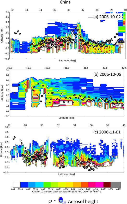
2258                                  J. Chimot et al.: Spatial pattern OMI aerosol layer height – comparison to CALIOP

is heavily investing in the development of polar-orbiting and      itoring Experiment-2 (GOME-2) and SCIAMACHY HCHO
geostationary satellite systems in the Copernicus program          (Barkley et al., 2012; Hewson et al., 2015), and about 50 %
(Ingmann et al., 2012), which will form an important com-          on OMI SO2 (Krotkov et al., 2008). ALH also remains one
ponent of air quality and climate observing systems on ur-         of the largest error sources for greenhouse gas retrievals:
ban, regional, and global scales (Martin, 2008; Duncan et al.,     e.g. CO2 from the American carbon OCO-2 mission (Crisp,
2014). However, inaccurate aerosol correction on these satel-      2015; Connor et al., 2016; Wunch et al., 2017) and CH4
lite measurements leads to misinterpretations and incorrect        from the future TROPOMI on board Sentinel-5 Precursor
evaluations of the implemented emission regulation controls.       (Hu et al., 2016).
   The magnitude of the radiative forcing by aerosols de-             Consequently, determining ALH with a large coverage
pends on the environmental conditions, aerosol properties,         (ideally daily and global) and an uncertainty better than
and horizontal and vertical distribution (IPCC: The Core           1 km (as a first approximation), for every single absorbing
Writing Team Pachauri and Meyer, 2014; Kipling et al.,             trace gas atmospheric satellite pixel, is ideally needed. Ac-
2016). Its determination requires satellite data in addition to    tive satellite sensors, such as the Cloud-Aerosol Lidar with
models (IPCC: The Core Writing Team Pachauri and Meyer,            Orthogonal Polarization (CALIOP), allow us to probe de-
2014). While, overall, the horizontal distributions of aerosol     tailed vertical aerosol profile, but with a limited coverage as
optical depth (AOD or τ ) and size are relatively well con-        they only look towards the nadir. This can lead to a gap up to
strained, uncertainties in vertical profile significantly con-     2200 km (in the tropics and subtropics) between adjacent or-
tribute to the overall uncertainty of radiative effects: e.g.      bital tracks. As an alternative, passive satellite sensors, with
25 % of the uncertainty of black carbon radiative estimations      a high spectral resolution such as OMI, offer adequate spatial
from the models is related to an inaccurate knowledge on           coverage with a good temporal resolution (up to daily global
the vertical distribution (McComiskey et al., 2008; Loeb and       before the OMI row anomaly development) thanks to a wide
Su, 2010; Zarzycki and Bond, 2010; IPCC: The Core Writing          swath. Thus, passive hyperspectral instruments can provide
Team Pachauri and Meyer, 2014). Knowledge of aerosol ver-          great contribution even if they do not achieve the same level
tical profiles allows the computation of related heating rates:    of accuracy as active instruments (i.e. limited vertical reso-
e.g. particles located above clouds can increase the liquid        lution, only cloud-free scenes). Because molecular oxygen
water path and geometric thickness of clouds and the subse-        (O2 ) is well mixed, its slant column measurement provides
quent atmospheric heating, and advection of light-absorbing        a suitable proxy for the determination of the modified scatter-
aerosols over the ocean and clouds from rice straw burning         ing height due to aerosols, in the absence of clouds. Most of
in China can strongly reduce clouds and Earth radiant energy       the developed ALH retrieval algorithms from backscattered
(Hsu et al., 2003; de Graaf et al., 2012; Wilcox, 2012). There-    sunlight satellite measurements focus on the absorption spec-
fore, aerosol layer height (ALH) drives not only the magni-        troscopy of the O2 A band around 765 nm, relatively close
tude but also the sign of aerosol direct and indirect radiative    to the CO2 and CH4 absorption bands (Wang et al., 2012;
effects (Kipling et al., 2016). Current ALH simulated by cli-      Sanders et al., 2015). Some studies also focus on the use of
mate models can differ in the range of 1.5–3 km (Koffi et al.,     the O2 B band (Ding et al., 2016; Xu et al., 2017). So far,
2012; Kipling et al., 2016).                                       only a few studies have worked on using the O2 −O2 satel-
   Furthermore, in the absence of clouds, vertical distribu-       lite absorption bands, within the ultraviolet (UV) and visi-
tion of aerosols is one of the most significant error sources      ble (vis) spectral ranges, to retrieve ALH and τ (Park et al.,
in trace gas retrievals from satellites (Leitão et al., 2010;      2016; Chimot et al., 2017). These bands are spectrally closer
Chimot et al., 2016). Major biases on the pollutant tropo-         to the NO2 , SO2 , and HCHO absorption lines. Contrary to the
spheric NO2 measured by satellites, depending on AOD and           O2 A band, the O2 −O2 477 nm band presents a wider (over
ALH, can be expected if no aerosol correction is applied. Be-      10 nm) but weaker spectral absorption. This leads to high
cause such information is not available for every observation,     sensitivities in the case of strong aerosol loading and less
aerosols are approximated via a simple cloud model (Acar-          challenges due to saturation. Moreover, in the visible spectral
reta et al., 2004; Boersma et al., 2011; Veefkind et al., 2016).   range, AOD values are generally higher while surface albedo
This only leads to a first-order correction for short-lived        or reflectance is lower, leading to a higher contrast between
gases (NO2 , SO2 , and HCHO) that does not comprehensively         aerosol and surface scattering signals. The 477 nm O2 −O2
assume the full scattering and absorbing effects of aerosol        channel is not only present in the current GOME-2, OMI,
particles on the average light path followed by the detected       and TROPOMI satellite sensors, but will be also included in
photons (Boersma et al., 2011; Chimot et al., 2016). In par-       future Sentinel-4 and Sentinel-5 instruments (Ingmann et al.,
ticular, current uncertainties on ALH lead to substantial bi-      2012; Veefkind et al., 2012).
ases in areas with high AOD (τ (550 nm) ≥ 0.5) and absorb-            This paper follows the exploratory study of Chimot et al.
ing and elevated particles: between −26 and −40 % on the           (2017), in which a neural network (NN) algorithm was devel-
retrieved tropospheric NO2 columns from the Dutch–Finnish          oped to investigate the feasibility of deriving ALH from the
Ozone Monitoring Instrument (OMI) (Castellanos et al.,             OMI 477 nm O2 −O2 spectral band over cloud-free scenes.
2015; Chimot et al., 2016), 20–50 % on Global Ozone Mon-           The main objective was the study of anthropogenic particles

Atmos. Meas. Tech., 11, 2257–2277, 2018                                              www.atmos-meas-tech.net/11/2257/2018/
J. Chimot et al.: Spatial pattern OMI aerosol layer height – comparison to CALIOP                                             2259

emission and their precursors from vehicles, coal burning,         2.2   The OMI aerosol layer height neural network
and industries. It has allowed us to retrieve ALH over land              algorithm
for the first time from this specific spectral band. A statistic
evaluation of 3-year cloud-free OMI observations over east-        The OMI ALH retrieval algorithm (Chimot et al., 2017) is
ern Asia, focusing on urban and large industrialized areas,        based on the exploitation of NOs 2 −O2 derived from the DOAS
has shown maximum differences below 800 m with a ref-              fit and relies on a NN approach. Here, the main elements
erence climatology database. In order to complete this first       of this algorithm are summarized, but for more details about
and statistically focused evaluation, the present study evalu-     their technical development and implementation, see Chimot
ates the spatial distribution of the OMI 477 nm O2 −O2 ALH         et al. (2017).
product on a pixel-by-pixel basis. It therefore focuses on its        This algorithm relies on how aerosols affect the length
variability for single days. For that purpose, specific cloud-     of the average light path along which the O2 −O2 absorbs.
free case studies are selected, including 3 winter days with       NOs 2 −O2 is then driven by the overall shielding or enhance-
strong anthropogenic pollution over eastern China. In addi-        ment effect of photons by the O2 −O2 complex in the visible
tion, to extend the performance assessment of such an ap-          spectral range due to the presence of particles. An aerosol
proach beyond the initial objective of Chimot et al. (2017),       layer located at high altitudes applies a large shielding ef-
new types of aerosol pollution episodes are investigated: 4        fect on the O2 −O2 located in the atmospheric layers below:
summer days with large biomass burning events in South             i.e. the amount of photons coming from the top of the atmo-
America and east of Russia and 1 day of wide desert dust           sphere (TOA) and reaching the lowest part of the atmosphere
transport over sea. The OMI ALH retrieval is compared with         is reduced compared to an aerosol-free scene. This shielding
the collocated CALIOP level 1 (L1) measurements and level          effect is then larger when the aerosol layer is located at an
2 (L2) aerosol retrievals.                                         elevated altitude than close to the surface.
                                                                      The designed NNs belong to the family of machine learn-
                                                                   ing and the artificial intelligence domain and rely on a multi-
                                                                   layer architecture, also named multilayer perceptron. The in-
2     OMI, MODIS, and CALIOP aerosol observations                  put and output variables are interconnected through a set of
                                                                   sigmoid functions present in the hidden layers and the synap-
2.1    The OMI sensor and O2 –O2 477 nm spectral band              tic weights W . For each single sigmoid function, two simple
                                                                   operations are performed: (1) a weighted sum of all the in-
The Dutch–Finnish OMI mission (Levelt et al., 2006) is             puts given by the previous layer and (2) a transport of this
a nadir-viewing push-broom imaging spectrometer launched           sum through the sigmoid functions. The ALH retrieval prob-
on the National Aeronautics and Space Administration               lem then becomes a simple series of analytical functions.
(NASA) Earth Observing System (EOS) Aura satellite. It de-            For all the processed OMI scenes, aerosol profile is as-
livers global coverage with a high temporal resolution of key      sumed as one single scattering layer (also called “box layer”)
air quality components derived from measurements of the            with a constant geometric thickness (100 hPa, or about 1 km).
backscattered solar radiation acquired in the UV–vis spectral      The particles included in this layer are homogeneous (i.e.
domain (270–550 nm) with approximately 0.5 nm resolution.          same size and optical properties). ALH is then defined as
Based on a two-dimensional detector array concept, radi-           the mid-altitude (a.s.l.) of this scattering layer. Furthermore,
ance spectra are simultaneously measured on a 2600 km wide         aerosol particles are assumed to cover the entire satellite ob-
swath within a nadir pixel size of 13 × 24 km2 (28 × 150 km2       servation pixel. The input layer contains seven parameters:
at extreme off-nadir).                                             viewing zenith angle θ , solar zenith angle θ0 , relative azimuth
   The O2 −O2 477 nm absorption band is currently opera-           angle φr , surface pressure P s, surface albedo A, aerosol opti-
tionally exploited by the OMI O2 −O2 cloud algorithm (OM-          cal thickness τ (550 nm), and the OMI NOs 2 −O2 . As explained
CLDO2) to derive effective cloud parameters (Acarreta et al.,      in Chimot et al. (2017), a prior τ (550 nm) is required as input
2004; Veefkind et al., 2016). This spectral band directly mea-     as both ALH and τ (550 nm) simultaneously affect NOs 2 −O2
sures the absorption of the visible part of the sunlight in-       and need to be distinguished.
duced by the O2 –O2 collision complex along the whole light           The optimal weights were estimated through a rigorous
path. A spectral fit, prior to the OMI effective cloud re-         training task following the error back propagation technique
trieval algorithm, is performed over the 460–490 nm spec-          and a training dataset that includes a set of representative sit-
tral range to derive the continuum reflectance Rc (475 nm)         uations for which inputs and outputs are well known. The
and the O2 −O2 slant column density NOs 2 −O2 . This spectral      quality of the training dataset was ensured by full physical
fit relies on the differential optical absorption spectroscopy     spectral simulations, dominated by aerosol particles with-
(DOAS) approach (Platt and Stutz, 2008). NOs 2 −O2 represents      out clouds, generated by the Determining Instrument Speci-
the O2 −O2 absorption magnitude along the average light            fications and Analyzing Methods for Atmospheric Retrieval
path through the atmosphere. This is the key input variable        (DISAMAR) software of KNMI (de Haan, 2011). Aerosol
for the OMI ALH retrieval by the NN algorithm.                     scattering is simulated by a Henyey–Greenstein (HG) scat-

www.atmos-meas-tech.net/11/2257/2018/                                                Atmos. Meas. Tech., 11, 2257–2277, 2018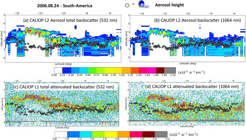
2260                                  J. Chimot et al.: Spatial pattern OMI aerosol layer height – comparison to CALIOP

tering phase function 8(2) parameterized by the asymme-           demanding and beyond the scope of this paper. Instead, more
try parameter g, which is the average of the cosine of the        elements on specific error analysis are further discussed in
scattering angle (Hovenier and Hage, 1989). Aerosols were         Sect. 4.
specified for a standard case, assuming fine particles with          Maximum seasonal differences between the LIdar cli-
a unique value of the extinction Ångström exponent α = 1.5        matology of Vertical Aerosol Structure for space-based li-
and g = 0.7. In order to investigate the assumptions related to   dar simulation studies (LIVAS) and 3-year OMI ALH,
the aerosol single scattering albedo ω0 properties, two train-    over cloud-free scenes in north-eastern Asia with MODIS
ing datasets were generated with a different typical value:       τ (550 m) ≥ 1.0, are in the range of 180–800 m (Amiridis
one with ω0 = 0.95 and one with ω0 = 0.9 in the visible spec-     et al., 2015; Chimot et al., 2017). The previous extended sen-
tral domain. Therefore, two OMI ALH NN algorithms were            sitive study has shown the following. (a) Due to the nature
created, one for each aerosol ω0 values.                          of the O2 −O2 spectral band, a minimum particle load (i.e.
   The aerosol models in the training database were based         τ (550 nm) = 0.5) is required to be able to exploit the aerosol
on a HG scattering phase function for two reasons. First,         signal as, below this threshold, low amounts of aerosols have
both Chimot et al. (2017) and this paper are exploratory stud-    negligible impacts on NOs 2 −O2 shielding and lead to high
ies focusing on the potential of exploiting the O2 −O2 spec-      ALH bias. (b) The aerosol model assumptions are the most
tral band for aerosol retrievals from a satellite sensor. Sec-    critical, in particular ω0 , as they may affect ALH retrieval un-
ond, our first long-term objective is the potential use of the    certainty up to 660 m. (c) In addition, potential aerosol resid-
ALH parameter for future tropospheric NO2 and similar trace       uals in the prior surface albedo may impact up to 200 m. (d)
gas retrievals over cloud-free scenes. Several studies empha-     An accuracy of 0.2 is required on prior τ (550 nm) to limit
sized that ALH is the key variable affecting the length of        ALH bias close to zero when τ (550 nm) ≥ 1.0 and below
the average light path in the computation of the related air      500 m for τ (550 nm) values close to 0.6.
mass factor (AMF) computation through the DOAS approach
(Boersma et al., 2004; Castellanos et al., 2015; Chimot et al.,   2.3   The CALIOP and MODIS aerosol products
2016). This is because the only quantity that is relevant for
absorption by trace gases in the visible is the average light     CALIOP sensor is a standard dual-wavelength elastically
path distribution, i.e. the distribution of distances travelled   backscattered lidar on board the CALIPSO satellite platform,
by photons in the atmosphere before leaving the atmosphere.       flying since 2006. Equipped with a depolarization channel at
The absolute radiance at the TOA is less important. The sec-      532 nm, it probes the aerosol and cloud vertical layers, from
ond variable of interest is τ . This average light path distri-   the surface to 40 km a.s.l., with a high vertical resolution
bution is mostly governed by ω0 and g, and of course ALH          (Winker et al., 2009). Level 1 scientific data products, dis-
and τ , and much less by details in the phase function. Studies   tributed by the Atmospheric Science Data Center (ASDC) of
by Leitão et al. (2010), Castellanos et al. (2015), and Chimot    NASA, include the lidar calibrated and geolocated measure-
et al. (2016) showed the lower sensitivity of the AMF to α,       ments of high-resolution vertical profiles (between 30 and
ω0 , and g. These scattering parameters are included in HG        60 m in the troposphere) of the aerosol and cloud attenuated
scattering, and therefore this parameterized phase function       backscatter coefficients at 532 and 1064 nm with horizontal
can be used for AMF calculations. At this level and with re-      resolutions of 1/3, 1, and 5 km (Winker et al., 2009).
spect to these mentioned objectives, it is then assumed one          The CALIOP aerosol L2 product contains the retrieved
does not need to define more realistic aerosol models for         aerosol backscatter and extinction coefficient profiles at 532
every single OMI pixel. With g = 0.7, the HG function is          and 1064 nm, for each identified and well-located aerosol
known to be smooth and reproduce the Mie scattering func-         layer, at 5 km horizontal resolution. These retrievals are
tions reasonably well for most of aerosol types, in partic-       performed after calibration, range correction, feature detec-
ular for spherical particles (e.g. nitrate, sulfate) (Dubovik     tion and classification, and assumptions on lidar extinction-
et al., 2002). Such an approach is used for the preparation       to-backscattering ratio (Winker et al., 2009; Young and
of the operational ALH retrieval algorithms for Sentinel-4        Vaughan, 2009).
and Sentinel-5 Precursor (Leitão et al., 2010; Sanders et al.,       The MODIS spectrometer was launched on the NASA
2015; Colosimo et al., 2016; Nanda et al., 2018) and for vari-    EOS Aqua platform in May 2002 and has been delivering
ous explicit aerosol corrections in the AMF calculation when      continuous images of the Earth in the visible, solar, and ther-
retrieving trace gases, such as tropospheric NO2 , over urban     mal infrared approximately 15 min prior to OMI. The consid-
and industrial areas dominated by anthropogenic pollution,        ered Aqua MODIS L2 aerosol product is the Collection 6 of
for example in eastern China (Spada et al., 2006; Wagner          MYD04_L2, based on the Dark Target (DT) and Deep Blue
et al., 2007; Castellanos et al., 2015; Vlemmix et al., 2010).    (DB) algorithms with a high enough quality assurance flag
The potential impact of the modelled scattering phase dis-        and an improved calibration of the instrument (Levy et al.,
cussion is kept in mind and further discussed in Sect. 4.4.       2013). While the MODIS measurement is acquired at the
However, reperforming the whole NN training process with          resolution of 1 km, the used MODIS aerosol τ (550 nm) is
more complex particle shape models is computationally very        at 10 km × 10 km, relatively close to the OMI nadir spatial

Atmos. Meas. Tech., 11, 2257–2277, 2018                                             www.atmos-meas-tech.net/11/2257/2018/
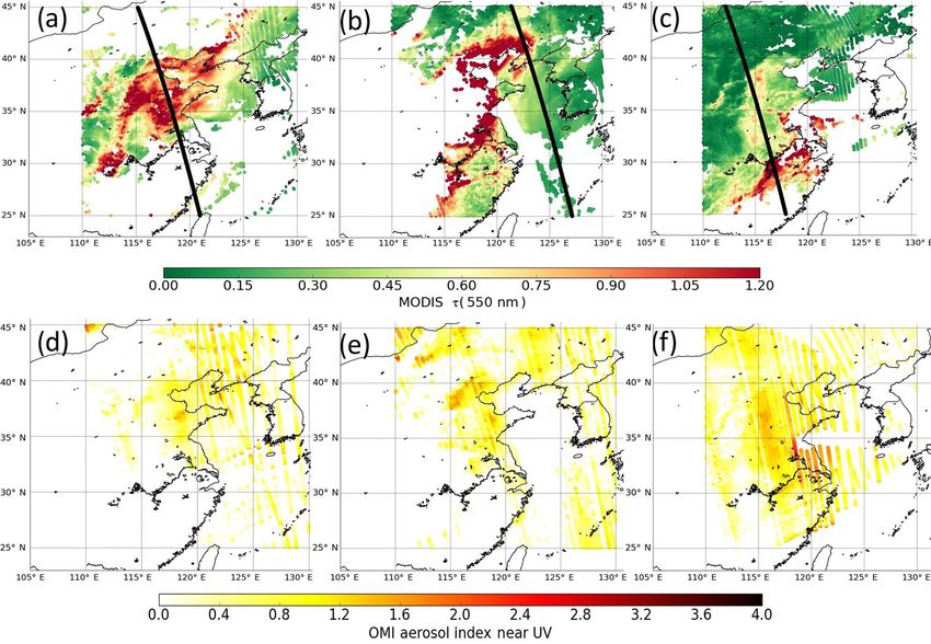
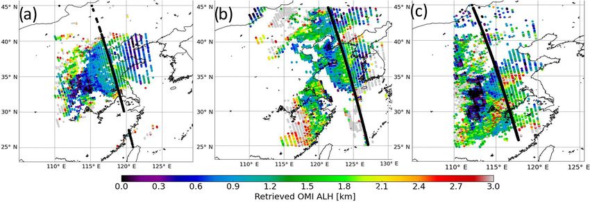
J. Chimot et al.: Spatial pattern OMI aerosol layer height – comparison to CALIOP                                                      2261

Figure 1. Maps of Aqua MODIS τ (550 nm) from the combined DT and DB Collection 6 (see Sect. 2.3) and collocated OMI aerosol index
from near-UV (UVAI) values (see Sect. 3) over cloud-free scenes for the urban and industrialized cases in eastern China. The dark thick lines
represent the track of CALIPSO space-borne sensor over the selected case studies: (a, d) 2 October 2006, (b, e) 6 October 2006, and (c, f)
1 November 2006.

Figure 2. Maps of retrieved OMI aerosol layer height (ALH) from all the cloud-free pixels collocated with Aqua MODIS τ (550 nm) (see
Fig. 1). The dark thick lines represent the track of CALIPSO space-borne sensor over the selected case studies: (a) 2 October 2006, (b)
6 October 2006, and (c) 1 November 2006.

www.atmos-meas-tech.net/11/2257/2018/                                                       Atmos. Meas. Tech., 11, 2257–2277, 2018
2262                                  J. Chimot et al.: Spatial pattern OMI aerosol layer height – comparison to CALIOP

resolution. The expected uncertainties of MODIS τ (550 nm)
are about ±0.05 + 15 % over land for DT (Levy et al., 2013)
and about ±0.03 on average for DB (Sayer et al., 2013).

3     Case studies: results and discussion

3.1    Methodology

OMI ALH retrievals are here obtained using MODIS L2
aerosol τ (550 nm) from the combined DT and DB product as
prior input, collocated within a distance of 15 km and where
τ (550 nm) ≥ 0.55 (see Sect. 2.2). Mitigating the probability
of cloud contamination within the OMI pixel is one of the
first criteria for a successful ALH retrieval. For that purpose,
we rely on the availability of the MODIS aerosol product
with the highest quality assurance flag ensuring that Aqua
MODIS τ (550 nm) is exclusively estimated when a sufficient
high amount of cloud-free sub-pixels is available (i.e. at the
MODIS measurement resolution of 1 km) (Levy et al., 2013).
However, since this may be not completely representative of
the atmospheric situation of the OMI pixel, two thresholds
are added for each collocated OMI–MODIS pixel: the geo-
metric MODIS cloud fraction to be smaller than 0.1, and the
effective OMI cloud fraction lower than 0.2. For this last pa-
rameter, it was shown that values higher than 0.3 are gener-
ally likely contaminated by clouds, while values between 0.1
and 0.2 may be cloud-free but contain a substantial amount
of very scattered particles that increase the scene brightness
(Boersma et al., 2011; Chimot et al., 2016).
   The ALH retrievals are applied to the OMI DOAS O2 −O2
observations, available in the last reprocessed OMCLDO2
                                                                   Figure 3. Retrieved OMI ALH compared with vertical profile of
product version (Acarreta et al., 2004; Veefkind et al., 2016).
                                                                   aerosol total backscatter coefficient (532 nm) from the CALIOP
A temperature correction is taken into account on the NOs 2 −O2    L2 product. Maximal distance between OMI pixels and CALIOP
variable, using the information available in the OMCLDO2           ground track is 50 km. Only cloud-free OMI pixels, collocated with
product, which is itself based on the temperature profiles of      Aqua MODIS Collection 6 aerosol cells, τ (550 nm) ≥ 0.55 (from
the National Centers for Environmental Prediction (NCEP)           the MODIS DT and DB algorithms), are selected: (a) 2 Octo-
analysis data (Veefkind et al., 2016).                             ber 2006, (b) 6 October 2006, and (c) 1 November 2006.
   The selected case studies include (1) urban and industrial
aerosol pollution over eastern China during 3 days between
October and November 2006, (2) large wildfire episodes in             For each study case, the most likely suitable NN algorithm
South America in August 2006 and September 2007 and in             (see Sect. 2.2) is selected by hand. We decided to rely on (1)
eastern Russia in August 2010 and June 2012, and (3) a Saha-       the OMI UV aerosol absorbing index (UVAI) and (2) their
ran dust transport over sea in June 2012. OMI ALH retrievals       well-known absorbing properties (according to the literature)
are compared with collocated CALIOP products within a dis-         in the visible spectral range in order to approximate the as-
tance of 50–100 km for the cases over eastern China and            sumption on aerosol ω0 at the visible (460–490 nm) spec-
South America and 300 km for eastern Russia. The larger            tral wavelengths. OMI UVAI is derived by the OMI near-UV
OMI–CALIOP distance over these two last regions is due             aerosol algorithm (OMAERUV) in the 330–388 nm spec-
to the so-called “row anomaly”, which has been significantly       tral band (Torres et al., 2007). It allows us to detect and
perturbing OMI measurements of the earthshine radiance at          distinguish UV absorbing from scattering aerosols through
all wavelengths since 2009. This leads to a reduced number         the measured change of spectral contrast, with respect to
of valid OMI ground pixels close to the CALIOP track. De-          a pure Rayleigh atmosphere. Weakly absorbing or large non-
tails are given at http://www.knmi.nl/omi/research/product/        absorbing particles are associated with near-zero or negative
rowanomaly-background.php (last access: 8 August 2010).            UVAI values. A threshold of 1 on UVAI is then specified to

Atmos. Meas. Tech., 11, 2257–2277, 2018                                               www.atmos-meas-tech.net/11/2257/2018/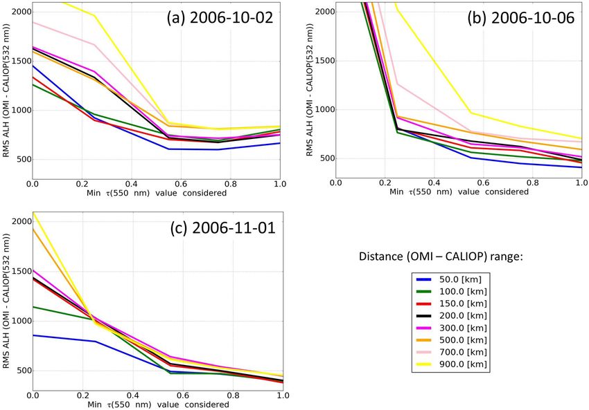
J. Chimot et al.: Spatial pattern OMI aerosol layer height – comparison to CALIOP                                            2263

Figure 4. Root-mean-square (RMS) deviation between collocated retrieved OMI ALH and derived CALIOP ALH (532 nm) (see Sect. 4.1)
for urban and industrialized cases over eastern China as a function of minimum MODIS τ (550 nm) and distance between OMI and CALIOP
ground pixels: (a) 2 October 2006, (b) 6 October 2006, and (c) 1 November 2006.

detect absorbing particles in the UV and then potentially in        of the NN algorithm over scenes with strong urban aerosol
the visible.                                                        pollution: day 1 of 2 October 2006, day 2 of 6 October 2006,
                                                                    and day 3 of 1 November 2006. As illustrated by the maps
3.2   Urban aerosol pollution                                       in Fig. 1, these days are characterized by high τ values over
                                                                    land as shown by Aqua MODIS: τ (550 nm) in the range of
                                                                    0.5–1.6 in October 2006, and 0.5–1.3 in November 2006. Lin
Fossil-fuel combustion is the main source of air pollution
                                                                    et al. (2015) estimated ω0 values in summer (and likely be-
in the large urban and industrialized area of eastern China.
                                                                    ginning of autumn) in the range of 0.94–0.96 in the visible.
With decreasing temperatures in autumn, coal-burning power
                                                                    This is likely a consequence of lower black carbon particle
plant activity is increased due to a higher energy consump-
                                                                    amounts at that time (compared to winter and spring) and
tion of heating systems. Consequently, excessive amounts of
                                                                    a high dominance of anthropogenic particles such as nitrate
aerosol particles and their precursors are emitted (Chamei-
                                                                    and sulfate. These particles may also be mixed, in parts, with
des et al., 1999). Moreover, crop residue burning in the agri-
                                                                    desert dust. Consistently, OMI UVAI depicts for the selected
cultural areas of eastern Asia may enhance aerosol concen-
                                                                    days values lower than or close to 1 (see Fig. 1). Therefore,
trations (Xue et al., 2014). Mineral dust particles, from the
                                                                    we use the NN algorithm trained with ω0 = 0.95 assuming
Taklamakan and Gobi deserts between middle of spring and
                                                                    low abundance of UV and visible absorbing particles.
end of autumn, are transported through westerly winds (Eck
                                                                       Figure 2 depicts the spatial distribution of retrieved OMI
et al., 2005; Proestakis et al., 2017). Collectively, the mix of
                                                                    ALH for all the selected collocated OMI–MODIS pixels,
all these pollutants contributes to the formation of regional
                                                                    with a variability between 0.5 and 3 km. The CALIPSO sub-
brown hazes greatly threatening public health, over the North
                                                                    orbital tracks were mostly located inland in days 1 and 3 and
China Plain during the dry season (from October to March).
                                                                    between inland and over sea in day 2 (see Fig. 1 and Fig. 2).
They have been frequently detected by satellite and ground-
                                                                    The aerosol layers in the CALIOP L2 product, based on the
based observations (Ma et al., 2010).
                                                                    total backscatter coefficients (532 nm), are generally located
   Three typical days between October and November 2006
                                                                    between the surface and 1.5 km height (see Fig. 3). Maxi-
in eastern China were selected to illustrate the performance

www.atmos-meas-tech.net/11/2257/2018/                                                Atmos. Meas. Tech., 11, 2257–2277, 2018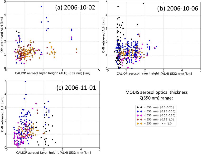
2264                                      J. Chimot et al.: Spatial pattern OMI aerosol layer height – comparison to CALIOP

Figure 5. Scatter-plot of collocated retrieved OMI ALH and derived CALIOP ALH (532 nm) (see Sect. 4.1) for urban and industrialized
cases over eastern China as a function of MODIS τ (550 nm). Distance between OMI and CALIOP pixels is 50 km: (a) 2 October 2006, (b)
6 October 2006, and (c) 1 November 2006.

mum top heights do not exceed 2 km on 6 October 2006 or             where σ (l) is the CALIOP aerosol extinction (532 nm) of the
3 km on the 2 other days. Collocated OMI ALH are mostly             vertical layer l defined by its mid-altitude h(l).
located in the middle aerosol layers and rarely exceed the             In Fig. 4, root-mean-square deviation (RMSD) between
top and bottom layer limits (see Fig. 2). Overall, for the 3        OMI and CALIOP L2 ALH lies in the range of 462–648 m
selected days, the OMI NN retrievals reproduce the spatial          when the maximum distance between the selected OMI and
CALIOP L2 patterns. On 2 October 2006 in particular, OMI            CALIOP ground pixels is lower than 50 km and with collo-
ALH remains relatively stable at the average altitude of 1 km,      cated MODIS τ (550 nm) ≥ 0.55 (see Fig. 3). Associated bias
within the CALIOP L2 aerosol layers (see Fig. 3a). Only at          values (i.e. average difference between OMI and CALIOP
the latitude 36.5◦ N do both products simultaneously show           ALH per day) are between −86 and −128 m. These re-
an increased altitude close to 3 km. On the 2 other selected        sults significantly deteriorate, firstly when specifying a lower
days, OMI ALH and CALIOP L2 show simultaneously de-                 threshold on collocated MODIS τ (550 nm) (e.g. RMSD ≥
scending slopes from south to north: a slope of about 2 km          1000 m with all MODIS τ (550 nm) values included) and sec-
over 2.5◦ latitude on 6 October 2006 and around 1.5 km over         ondly with a more flexible distance criterion (e.g. RMSD in
8◦ latitude on 1 November 2006 (see Fig. 3b and c).                 the range of 594–888 m with a maximum distance of 500 km
   An equivalent CALIOP L2 ALH can be derived by cal-               between the selected OMI and CALIOP ground pixels). The
culating an aerosol extinction weighted average altitude as         relatively low impact, noticed here, on the distance between
follows:                                                            OMI and CALIOP pixels is probably related to the large spa-
                                                                    tial extent of aerosol plumes and their relative spatial homo-
                       P                                            geneity. The impact of distance between collocated OMI–
                            h(l)σ (l)                               CALIOP pixels would be more detrimental over scenes with
                        l
ALH(CALIOP L2) =            P         ,                     (1)     smaller and/or more heterogeneous plumes. Figure 5 shows
                              σ (l)                                 the one-to-one comparison between OMI and CALIOP L2
                             l

Atmos. Meas. Tech., 11, 2257–2277, 2018                                               www.atmos-meas-tech.net/11/2257/2018/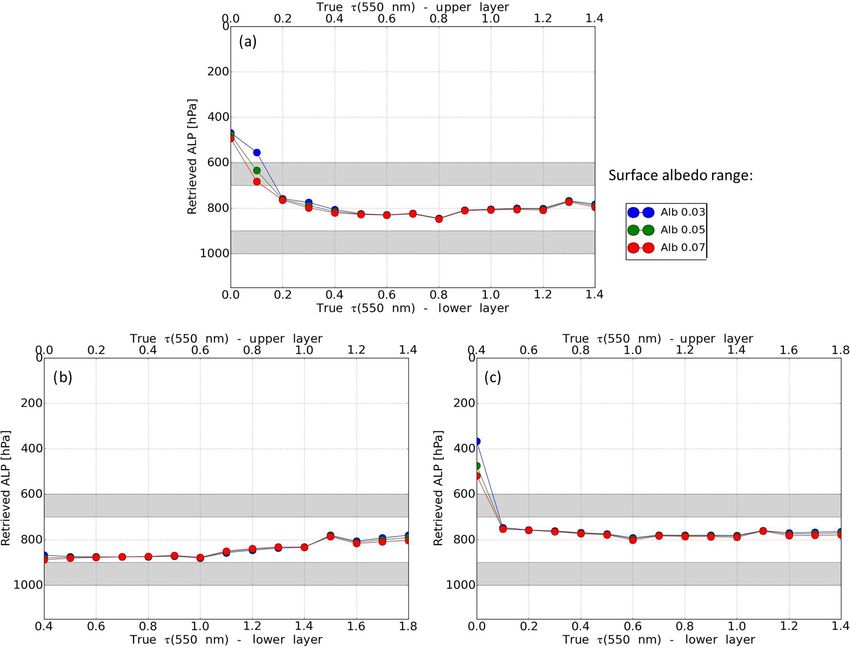
J. Chimot et al.: Spatial pattern OMI aerosol layer height – comparison to CALIOP 2265
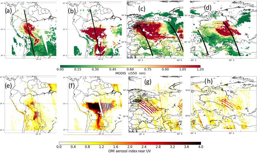
Figure 6. Maps of Aqua MODIS τ (550 nm) from the combined DT and DB Collection 6 (see Sect. 2.4) and collocated OMI aerosol index
from near-UV (UVAI) values (see Sect. 3) over cloud-free scenes and intensive biomass burning episodes. The dark thick lines represent
the track of CALIPSO space-borne sensor over the selected case studies: (a, e) South America on 24 August 2006, (b, f) South America on
30 September 2007, (c, g) eastern Russia on 8 October 2010, and (d, h) eastern Russia on 23 June 2012.
ALH within a distance of 50 km per case study and as a func- suggesting the use of the NN algorithm trained with ω0 = 0.9
tion of associated MODIS τ (550 nm). The correlation coef- (see Fig. 6).
ficient (R) between OMI and CALIOP ALH varies per day, Several studies have identified loss of sensitivity of
between 0.4 and 0.6 for all scenes with MODIS τ (550 nm) ≥ CALIOP attenuated backscatter profile measurements at
0.55. 532 nm over scenes with dense smoke layers, such as over
Canadian boreal and Amazonian fire events (Kacenelenbo-
gen et al., 2011; Torres et al., 2013; Wu et al., 2014). Light
3.3 Smoke and absorbing aerosol pollution from
extinction due to these layers is much larger at 532 nm than
biomass-burning
at 1064 nm (Pueschel and Livingston, 1990). Since CALIOP
does not directly measure the aerosol backscattering but
Intensive biomass burning releases large amounts of car- rather the attenuated backscattering, the range-dependent re-
bonaceous and black carbon aerosols. The resulting dense duction in CALIOP lidar signals due to attenuation occurs
smoke layers have a predominance of fine and strongly light- more rapidly in the short wavelengths. Therefore, over scenes
absorbing particles, especially in both the UV and visible with heavy smoke particle loads, the attenuated backscatter
spectral ranges. Combined with large τ values, this yields coefficients (532 nm) in the lower part of the aerosol layer
large light extinction and Ångström exponents (≥ 1.5) (Tor- fall below the CALIOP’s detection threshold, preventing the
res et al., 2013; Wu et al., 2014). Figure 6 shows the location identification of the full vertical extent of the aerosol layers
and associated MODIS τ (550 nm) and OMI UVAI values for (from the top to the bottom). Being a down-looking obser-
the selected biomass burning episodes: the two first events vation lidar system, CALIOP tends then to mostly detect the
are over South America on 24 August 2006 and 30 Septem- top height compared to the base height of the aerosol layer
ber 2007; the two last events are over eastern Russia on 8 Au- as the laser’s energy undergoes substantial attenuation when
gust 2010 and 23 June 2012. Due to the very high load of ab- the beam travels through an optically thick layer (Vaughan
sorbing particles with MODIS τ (550 nm ≥ 1.1), OMI UVAI et al., 2005; Kim et al., 2013). Therefore, the identified lay-
values are generally higher than 2 and can locally reach 4,
www.atmos-meas-tech.net/11/2257/2018/ Atmos. Meas. Tech., 11, 2257–2277, 2018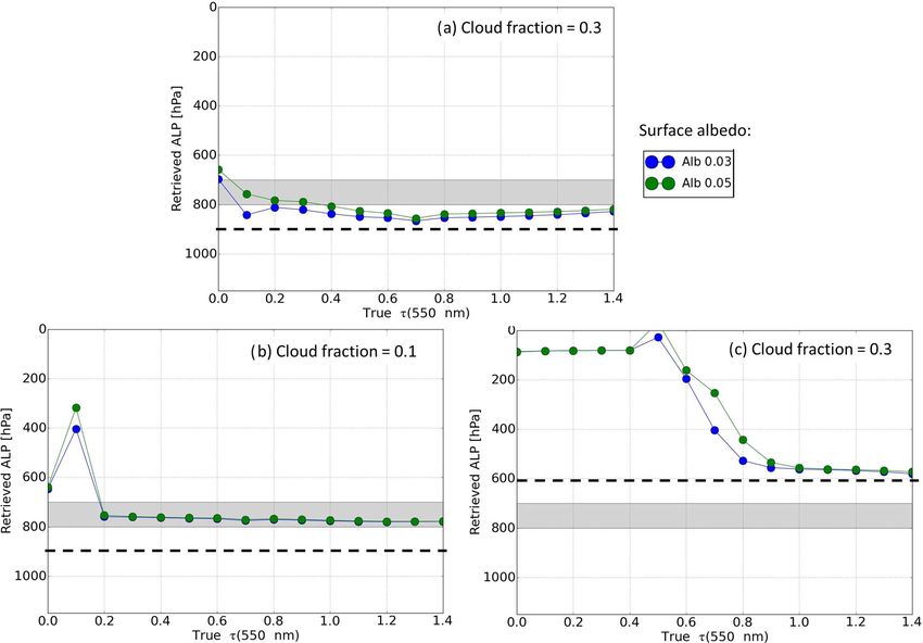
2266                                  J. Chimot et al.: Spatial pattern OMI aerosol layer height – comparison to CALIOP

Figure 7. Retrieved OMI ALH compared with CALIOP along-track vertical profile observations for biomass burning case over South Amer-
ica: (a) CALIOP L2 aerosol total backscattering (532 nm), (b) CALIOP L2 aerosol backscattering (1064 nm), (c) CALIOP L1 attenuated
backscattering (532 nm), and (d) CALIOP L1 attenuated backscattering (1064 nm).

ers that are fully attenuated at 532 nm in the L1 product are       ond aerosol layer, close to the surface (see Fig. 7d). Contrary
filtered out in the L2 product. As a consequence of this fil-       to the CALIPSO L1 measurement (532 nm), our retrievals
tering, CALIOP’s τ of smoke layers is generally underesti-          based on OMI visible measurements are not restricted to the
mated due to an overestimation of the layer base altitude (Wu       top of the smoke or absorbing layer but correctly match with
et al., 2014; Kim et al., 2013).                                    the middle of the layers detected by CALIPSO L1 (1064 nm).
    Figure 7 depicts an example of the loss of sensitivity for      The reason that our OMI ALH seems closer to the top of the
a biomass burning case in South America. The CALIOP                 second layer may be due to a higher aerosol load and/or dif-
aerosol total backscatter (532 nm) and backscatter (1064 nm)        ferent layer properties (see Section 4.2).
coefficients in the L2 product mostly show the top layer               Figure 8 shows that similar full CALIOP attenuation pro-
of carbonaceous aerosols in the range of 3–4 km altitude            cesses occur with the other selected biomass burning cases.
with maximum thickness of 1 km, between 14 and 11◦ S                The CALIOP L1 total attenuated backscatter (532 nm) ver-
(see Fig. 7a and b). We found that the layers located be-           tical profiles mostly correlate with the top of the detected
low are flagged as totally attenuated at the wavelength of          aerosol layers, while the CALIOP L1 attenuated backscat-
532 nm, according to the CALIOP vertical feature mask. On           ter (1064 nm) profiles reveal lower layers. On days of
the northernmost end of the detected plume, the aerosol load        30 September 2007 and 8 August 2010, the top layers are
is around 2 km height. In contrast, the CALIOP L1 attenu-           at elevated altitudes (higher than 3 km), while the lower
ated backscatter (1064 nm) profile detects an aerosol layer         ones extend from the surface to 1–2 km. On the last day,
between the surface and 1.5 km, at the latitudes 11–14◦ S.          23 June 2012, the top layer is lower (between 1 and 2 km).
This layer is not observed by the CALIOP L1 total attenu-           Similarly, all the OMI ALH retrievals are not restricted to
ated backscatter (532 nm) profile (see Fig. 7c and d) likely        the top layers but match, most of the time, with the middle
due to a better sensitivity of this channel to the particles lo-    of the layers, sometimes a bit closer to the base of the top
cated close to the surface.                                         layer or the top of the bottom layer. This may depend on the
    The case of 24 August 2006 over South America shows the         differences in terms of AOD and/or optical properties of each
retrieved OMI ALH being well located, i.e. below the first el-      layer (see Sect. 4.2). In addition, it is worth noting the similar
evated aerosol layer (at about 3 km) and at the top of the sec-     vertical variability (around 500 m) on 30 September 2007 in

Atmos. Meas. Tech., 11, 2257–2277, 2018                                                www.atmos-meas-tech.net/11/2257/2018/
J. Chimot et al.: Spatial pattern OMI aerosol layer height – comparison to CALIOP 2267
Figure 8. Retrieved OMI ALH compared with CALIOP L1 along-track vertical profile observations (532 and 1064 nm) for biomass burning
cases: (a, b) 30 September 2007 in South America, (c, d) 8 August 2010 in eastern Russia, and (e, f) 23 June 2012 in eastern Russia.
South America at the latitudes 8–15◦ S and the remarkable tion threshold due to the large associated lidar ratio and thus
descending slope, on 23 June 2012 in eastern Russia, from low SNR (Winker et al., 2013).
north to south at the latitudes 56–58◦ S present in both OMI
ALH and CALIOP L1 products. 3.4 Desert dust transport
Three reasons may explain why OMI visible spectra al-
low us to probe an entire absorbing aerosol layer, contrary The case illustrated in Fig. 9a is a large desert dust plume
to the active satellite visible measurement of CALIOP: (1) over ocean surface, with MODIS τ (550 nm) values up to
OMI measurements rely on the sun irradiance, which is much 1.1, released from the Sahara and transported through west-
more intense than the laser pulse of CALIOP; (2) OMI mea- erly winds along the African coast. It occurred in summer
surements are largely issued from multiple scattering effects on 19 July 2007. Since the Sahara is the most important
occurring at different altitudes, allowing a higher number of source of mineral particles, associated dust aerosols include
photons to reach the lower atmospheric layers; (3) the rela- hematite and other iron oxides. Spectrally, desert dust is
tively higher signal-to-noise ratio (SNR) of OMI likely al- a UV-absorbing particle but quite highly scattering in the
lows us to better detect and exploit the upcoming signal from visible (contrary to smoke) and longer wavelengths, leading
smoke layers. In contrast, contributions of multiple scatter- to the appearance of relatively bright plumes (light brown)
ing to the CALIOP backscattered signals are lower than sin- over the dark marine surface from a satellite point of view.
gle scattering effects within moderately dense dust layer and The NN algorithm trained with aerosol ω0 = 0.95 is there-
insignificant within smoke aerosol extinction (Winker, 2003; fore used here.
Liu et al., 2011). Furthermore, retrieving vertical profile of The vertical profile of CALIOP L2 aerosol total backscat-
smoke layers from CALIOP requires a high aerosol extinc- ter (532 nm) shows elevated layers, ranging from 1–2 km at
15◦ S to 3–6 km at 23◦ S (see Fig. 9b). Such a slope likely
www.atmos-meas-tech.net/11/2257/2018/ Atmos. Meas. Tech., 11, 2257–2277, 20182268 J. Chimot et al.: Spatial pattern OMI aerosol layer height – comparison to CALIOP
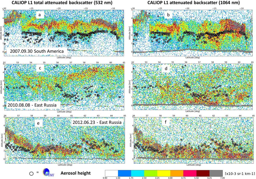
Figure 9. Elevated layer due to a Saharan dust outbreak transported to western Mediterranean region over sea on 19 July 2007. (a) Map
of Aqua MODIS τ (550 nm) from the combined DT and DB Collection 6 (see Sect. 2.3). (b) Retrieved OMI ALH compared with vertical
profile of aerosol total backscatter coefficient (532 nm) from the CALIOP L2 aerosol total backscatter (532 nm) associated with the second
left CALIPSO track over sea in Fig. 9a.
results from large-scale circulation governed by subtropical (i.e. non-spherical). Their optical modelling in the NN train-
subsidence of the Intertropical Convergence Zone’s northern ing dataset regarding their assumed size and the employed
branch, dry air from the desert, and the Saharan intense sensi- phase function model (see Sect. 2.2) may contribute to the
ble heating effect perturbing the temperature inversion layers higher ALH uncertainties than in urban cases of Sect. 3.2
and thus creating convection uplifting dust from the surface (see further discussions in Sect. 4.3 and 4.4).
(Prospero and Carlson, 1981). Generally, the OMI ALH re-
sults are consistent with CALIOP observations, with elevated
values lying between 2 and 7 km. They are mostly located 4 Specific error analysis
in the middle of the large uplifted dust plume from south
to north. The average difference between OMI and CALIOP The analysed OMI ALH in Sect. 3 may include uncertain-
L2 ALH, collocated within a distance of 100 km, is −350 m. ties due to assumptions made on the aerosol models used
However, OMI ALH depicts significant variabilities com- in the NN training dataset. The following subsections fo-
pared to CALIOP ALH. The SD of the related differences cus on some specific uncertainty sources that are relevant for
is therefore quite large, about 2.1 km. these specific case studies. They provide further detailed er-
Several elements likely contribute to the difficulties en- ror analysis and are complementary to the evaluations per-
countered in this case study. Desert dust particles can be rel- formed in (Chimot et al., 2017). Most of these analyses are
atively coarse (thus low α value) and are irregularly shaped based on synthetic scenarios. Simulations are performed in
a similar way as in the NN training dataset (see Sect. 2.2).
Atmos. Meas. Tech., 11, 2257–2277, 2018 www.atmos-meas-tech.net/11/2257/2018/J. Chimot et al.: Spatial pattern OMI aerosol layer height – comparison to CALIOP 2269
4.1 Aerosol single scattering albedo
Aerosol ω0 represents the scattering vs. absorption efficiency
of the particles and therefore directly drives the magnitude of
the applied shielding effect on the O2 −O2 dimers (Chimot
et al., 2016). An overestimated ω0 , in the training database,
directly leads to an overestimation of ALH (or underestima-
tion of ALP) as the measured NOs 2 −O2 is lower (i.e. stronger
shielding) than expected if one knows the true extinction pro-
file and assumes a biased ω0 (Chimot et al., 2017).
Dense smoke layers from wildfires, such as those analysed
in Sect. 3.2, may contain particles that are more absorbing
than the assumed aerosol model. Figure 10 illustrates the
impact of particles with ω0 = 0.8 while the NN algorithm
trained with ω0 = 0.9 is used (same as in Sect. 3.2). No er-
Figure 10. Simulated ALP retrievals, based on noise-free synthetic rors are introduced in all the other geophysical parameters.
spectra with aerosols, as a function of true τ (550 nm). All the re- The resulting ALP values are overestimated with a bias up
trievals are achieved with the NN algorithm trained with aerosol to 100 hPa (around 900 m) for scenes with τ (550 nm) in the
ω0 = 0.9 and true prior τ (550 nm) value. The assumed geophysi-
range of 0.5–0.9. ALP biases are almost null over scenes with
cal conditions are temperature, H2 O, O3 , and NO2 from climatol-
higher aerosol load as the shielding effect due to the already
ogy mid-latitude summer, θ0 = 25◦ , θ = 45◦ , and Ps = 1010 hPa.
The reference aerosol scenario assumes fine scattering particles high amount of particles clearly dominates over their optical
(α = 1.5, g = 0.7) and two aerosol ω0 values: 0.9 and 0.8. Its lo- properties. In these conditions, the shielding effect induced
cation is depicted by the grey box, between 700 and 800 hPa. by particles is less dependent on ω0 assumptions. These re-
sults are in line with those estimated from the use of the NN
algorithm trained with ω0 = 0.95 in Chimot et al. (2017).
4.2 Aerosol vertical distribution
Due to the specific limitations of passive satellite sensor,
the OMI ALH retrieval summarizes the description of the
aerosol extinction profile in a single scalar value, assuming
a specific profile shape. However, aerosol profiles in the ob-
served scene may considerably deviate from this simplified
profile description. It is then legitimate to ask the meaning
of the retrieved ALH. As explained in Sect. 2, the NNs were
trained based on a single “box layer” with a constant geomet-
ric thickness of about 1 km (100 hPa exactly), ALP (ALH)
being then the mid-pressure (mid-altitude) of this layer. Sev-
eral of the analysed cases in Sect. 3 depict more extended
aerosol layers (e.g. up to 3.5 km in Fig. 8b) or two separate
layers (e.g. Fig. 7b).
Figure 11. Same as Fig. 10 but with one unique aerosol ω0 value (= Figure 11 illustrates the retrievals in a case of an extended
0.9) and a larger geometric extension of the aerosol layer included aerosol layer with thickness of 300 hPa, located between 700
in the simulated spectra, i.e. between 700 and 1000 hPa. and 1000 hPa. The derived ALP values are close to 850 hPa
for scenes with τ (550 nm) ≥ 0.5, which thus corresponds to
the mid-level of the simulated layer. This result may be un-
derstood as the true aerosol vertical extinction profile being
No bias is introduced in the geophysical parameters such lower than the assumption. The retrieval then reaches the av-
as surface, temperature profile, and atmospheric trace gases. erage altitude where most of the O2 −O2 is actually shielded.
The true prior aerosol τ (550 nm) value is given for all the In Fig. 12, ALP is retrieved when two separate aerosol
retrievals. Aerosols are assumed to cover the full ground layers with same thickness (i.e. 100 hPa) are simulated: an
pixel. The key analysed variable is the aerosol layer pressure elevated one between 600 and 700 hPa and a lower one be-
(ALP), which corresponds to ALH expressed in hPa in order tween 900 and 1000 hPa. Assuming that both layers have
to be consistent with all the input parameter specifications same optical properties, ALP is retrieved close to 800 hPa
(e.g. vertical grid) in the radiative transfer simulations. for τ (550 nm) ≥ 0.5 (see Fig. 12a). Here, the retrieval corre-
www.atmos-meas-tech.net/11/2257/2018/ Atmos. Meas. Tech., 11, 2257–2277, 20182270 J. Chimot et al.: Spatial pattern OMI aerosol layer height – comparison to CALIOP
Figure 12. Same as Fig. 10 but with one unique aerosol ω0 value (= 0.9) and two separate aerosol layers included in the simulated spectra.
The bottom x axis corresponds to the τ (550 nm) value of the lower layer, while the top x axis is the τ (550 nm) value of the upper layer.
Both layers have same geometric thickness (i.e. 100 hPa). The first is located between 600 and 700 hPa, and the second is between 900 and
1000 hPa. (a) Both aerosol layers have same optical properties and τ (550 nm) values. (b) Both aerosol layers have same optical properties but
different τ (550 nm) values: the lower layer has systematically a higher τ (550 nm) (i.e. +0.4 for each scenario). (c) Both aerosol layers have
same optical properties but different τ (550 nm) values: the upper layer has systematically a higher τ (550 nm) (i.e. +0.4 for each scenario).
sponds to the average height of both layers. However, when 4.3 Aerosol size
one of these layers has a higher aerosol load (i.e. a higher
value for τ (550 nm)), the retrieval is close to the optically Within the HG phase function model, particle size is primar-
thicker aerosol layer for total τ (550 nm) in the range of 0.0– ily governed by α, which describes the spectral variation of
1.6 and reaches the average height (i.e. 850 hPa) for total the aerosol load τ . While the NNs were trained for fine par-
τ (550 nm) ≥ 1.6. This demonstrates the sensitivity of the re- ticles emitted from anthropogenic activities such as power
trieval to the extinction properties of the particles and its plants and vehicles (i.e. α = 1.5), other particles such as dust
vertical distribution driving the location where most of the can be coarser.
O2 −O2 dimers are shielded. As a consequence, the retrieved Figure 13 depicts the ALP retrievals assuming scattering
ALP and ALH actually represent a weighted average of the particles with ω0 = 0.95 (same as in Sect. 3.4) but with dif-
actual aerosol vertical distribution, the weights being the ex- ferent α values: 1.5 (consistent with the training dataset)
tinction values distributed along the vertical atmospheric lay- and 0.5. Overestimating α (i.e. underestimating particle size)
ers. leads to a increase (decrease) of retrieved ALP (ALH). This
is because coarser particles generally extend the length of
the average light path, due to reduced multiple scattering,
Atmos. Meas. Tech., 11, 2257–2277, 2018 www.atmos-meas-tech.net/11/2257/2018/J. Chimot et al.: Spatial pattern OMI aerosol layer height – comparison to CALIOP 2271
does reasonably well without additional biases than those
analysed in the previous sections.
Pure desert dust particles are known to be irregularly
shaped, and thus the use of the HG forward model may be
inappropriate in Sect.3.3 and Fig. 9. Furthermore, by using
a prior τ parameter from MODIS, that may also be derived
from an inaccurate and different model, can add some incon-
sistencies in the OMI ALH retrieval. This may explain in part
the larger uncertainties found in Sect.3.3. In further steps, to
confirm the real performances of ALH retrievals over a long
time series of OMI measurements and/or a potential imple-
mentation in the OMI processing chain, new NN algorithms
should be designed and trained with a larger dataset that in-
cludes accurate aerosol parameters (size and ω0 ) combined
with different detailed models of the phase function. Each of
Figure 13. Same as Fig. 10 but with one unique aerosol ω0 value these algorithms should be evaluated on a high number of
(= 0.95) and two aerosol α (1.5 and 0.5) in the reference aerosol specific observations to conclude on the exact aerosol model
scenarios. ALP retrievals are estimated from the NN algorithm type to be assumed for the OMI visible spectral measure-
trained with aerosol ω0 = 0.95 similarly to the desert dust case in ments.
Sect. 3.4.
4.5 Cloud contamination
lower the O2 −O2 shielding, and thus increase the measured When backscattered solar light measurements from UV–vis
NOs 2 −O2 as shown in Chimot et al. (2016). The ALP change passive satellite sensors are exploited, detecting cloud-free
is nevertheless about 25 hPa. pixels is one of the most crucial prerequisite for aerosol re-
trievals. In spite of a strict cloud filtering applied in Sect. 3.1,
4.4 Scattering phase function some small cloud residuals may remain in the analysed
scenes, especially over biomass burning episodes where the
Modelling the aerosol scattering phase function requires pre- distinction of dense smoke particles and small cloud layers
cise information not only on their size and optical proper- can be difficult.
ties but also on their shape and the phase function modelling Presence of cloud layers have similar effects as aerosols on
theory itself. As an example, optical modelling of desert the OMI visible measurements and the O2 −O2 molecules, al-
dust can, for some applications, be done using Mie theory, though associated optical thickness are an order of magnitude
which is mostly valid for homogeneous and spherical parti- higher. In Fig. 14, cloud layers were added to an aerosol layer
cles, whereas for other applications one could better consider located between 700 and 800 hPa. Clouds were simulated as
alternative spheroids or T-matrix/geometric optics tradition- an opaque Lambertian bright layer with an albedo of 0.8 and
ally used for non-spherical particles (de Graaf et al., 2007; different effective cloud pressure and fraction values. Such
Xu et al., 2017). a model is similar to what is employed in the OMCLDO2
For reasons explained in Sect. 2.2, the HG was employed algorithm to detect and characterize the presence of clouds
in the NN training database. This may lead to some errors within the OMI pixel or to implicitly correct aerosol effect
in ALH and ALP retrievals due to inaccurate scattering an- in trace gas retrievals (Acarreta et al., 2004; Veefkind et al.,
gular dependence, depending on the particle type and the as- 2016; Boersma et al., 2011; Chimot et al., 2016). It should
sumed g parameter. The shape of the phase function is pa- be noted that aerosols are assumed to cover the whole scene
rameterized by g in HG modelling, which reproduces well in the simulations.
the Mie scattering function and thus spherical particles. In Figure 14 shows that the impact on the ALP retrieval
Chimot et al. (2016), we demonstrated that bias on ALP strongly depends on the cloud altitude. If the aerosol layer
does not exceed 50 hPa for a typical uncertainty of 0.1 on is located below a cloud with an effective fraction of 0.3, the
g over scenes with τ (550 nm) ≥ 0.5, assuming no additional ALP is strongly biased low (i.e. ALH high) for τ (550 nm) ≤
bias on α or ω0 . Comparison between Mie and HG mod- 0.8, while it tends towards the effective cloud pressure for
elling would mix errors caused by these three parameters τ (550 nm) ≥ 0.8 (see Fig. 14c). Such a behavior may be ex-
altogether, which would then make complex to identify the plained by the high O2 −O2 shielding caused by the clouds,
actual error source. Colosimo et al. (2016) and Sanders et al. much higher than what is anticipated by the retrieval algo-
(2015) show with simulation studies comparing phase func- rithm through the given aerosol τ (550 nm). The assumed
tion models, although in different spectral bands, that using optical thickness of the scene is too low to match with
a scattering layer with constant particle extinction coefficient the strongly reduced NOs 2 −O2 measurement, especially over
www.atmos-meas-tech.net/11/2257/2018/ Atmos. Meas. Tech., 11, 2257–2277, 2018You can also read