Planetary boundary layer height by means of lidar and numerical simulations over New Delhi, India - Atmos. Meas. Tech
←
→
Page content transcription
If your browser does not render page correctly, please read the page content below
Atmos. Meas. Tech., 12, 2595–2610, 2019
https://doi.org/10.5194/amt-12-2595-2019
© Author(s) 2019. This work is distributed under
the Creative Commons Attribution 4.0 License.

Planetary boundary layer height by means of lidar and numerical
simulations over New Delhi, India
Konstantina Nakoudi1,2,3 , Elina Giannakaki1,4 , Aggeliki Dandou1 , Maria Tombrou1 , and Mika Komppula4
1 Department    of Environmental Physics and Meteorology, Faculty of Physics, University of Athens, Athens, Greece
2 Alfred  Wegener Institute, Helmholtz Centre for Polar and Marine Research, Potsdam, Germany
3 Institute of Physics and Astronomy, University of Potsdam, Potsdam, Germany
4 Finnish Meteorological Institute, Kuopio, Finland

Correspondence: Konstantina Nakoudi (knakoudi@phys.uoa.gr)

Received: 30 September 2018 – Discussion started: 20 November 2018
Revised: 28 March 2019 – Accepted: 30 March 2019 – Published: 6 May 2019

Abstract. In this work, the height of the planetary boundary      key component of the atmosphere and of the climate system,
layer (PBLH) is investigated over Gwal Pahari (Gual Pahari),      as it fundamentally affects cloud processes, as well as land
New Delhi, for almost a year. To this end, ground-based mea-      and ocean surface fluxes (Oke, 1988; Stull, 1988; Garratt,
surements from a multiwavelength Raman lidar were used.           1992). The PBL height (PBLH) is the most adequate param-
The modified wavelet covariance transform (WCT) method            eter to represent the PBL. Therefore, it is usually required in
was utilized for PBLH retrievals. Results were compared           numerous applications, for instance in pollution-dispersion
to data from Cloud-Aerosol Lidar and Infrared Pathfinder          modeling, where the upper boundary of the turbulent layer
Satellite Observation (CALIPSO) and the Weather Research          acts as an impenetrable lid for the pollutants emitted at the
and Forecasting (WRF) model. In order to examine the dif-         surface. The PBLH also appears as a mixing-scale height
ficulties of PBLH detection from lidar, we analyzed three         in turbulence closure schemes within climate and weather
cases of PBLH diurnal evolution under different meteorolog-       prediction models (Zilitinkevich and Baklanov, 2001). As
ical and aerosol load conditions. In the presence of multiple     air pollution becomes more severe due to economic devel-
aerosol layers, the employed algorithm exhibited high effi-       opment, particularly in developing countries (Wang et al.,
ciency (r = 0.9) in the attribution of PBLH, whereas weak         2009), high temporal and vertical resolution observations
aerosol gradients induced high variability in the PBLH. A         of the PBLH are essential for weather and air-quality pre-
sensitivity analysis corroborated the stability of the utilized   diction and research. Moreover, the PBLH is related to the
methodology. The comparison with CALIPSO observations             warming rate caused by enhanced greenhouse gas emissions
yielded satisfying results (r = 0.8), with CALIPSO slightly       (Pielke et al., 2007). Several methods have been proposed to
overestimating the PBLH. Due to the relatively warmer and         estimate the PBLH, utilizing vertically resolved thermody-
drier winter and, correspondingly, colder and rainier pre-        namic variables, turbulence-related parameters and concen-
monsoon season, the seasonal PBLH cycle during the mea-           trations of tracers (Seibert et al., 2000; Emeis et al., 2004).
surement period was slightly weaker than the cycle expected       Different methods for the determination of the PBLH from
from long-term climate records.                                   radiosondes have been compared and the associated uncer-
                                                                  tainties have been estimated (Seidel et al., 2010; Wang and
                                                                  Wang, 2014). Restrictions of radiosondes refer to the coarse
                                                                  vertical resolution of standard meteorological data with re-
1   Introduction                                                  spect to boundary layer studies as well as the smoothing
                                                                  due to the sensor lag constant bounded by the high ascent
The planetary boundary layer (PBL) is the lowermost portion       rate of the radiosonde (Seibert et al., 2000). Remote-sensing
of the troposphere, which experiences a diurnal cycle of tem-     systems such as aerosol lidar (Boers and Eloranta, 1986;
perature, humidity, wind and pollution variations. PBL is a

Published by Copernicus Publications on behalf of the European Geosciences Union.
2596                                              K. Nakoudi et al.: Planetary boundary layer height over New Delhi, India

Davis et al., 2000; Lammert et al., 2006; Lange et al., 2014),        Despite the importance of the area under investigation,
microwave radiometer (Cimini et al., 2013), wind-profiling         only a few ground-based measurements of aerosol vertical
radar (Cohn and Angevine, 2000) and Doppler wind lidar             profiles have been carried out, with most of the available data
(de Arruda Moreira et al., 2018) are suitable for long-term        accessed during short field campaigns (Lelieveld et al., 2001;
measurements of various atmospheric quantities with high           Nakajima et al., 2007; Ramanathan et al., 2007). In this study,
temporal resolution and can be used either independently           we investigate PBLH characteristics over New Delhi, In-
or synergistically to retrieve the PBLH. Space-borne lidar         dia, based on 1-year-long ground-based lidar measurements.
systems provide the advantage of spatial coverage, although        The measurements were carried out from March 2008 to
for studies focusing on a particular area of interest, mea-        March 2009 in the framework of the EUCAARI (European
surements are constrained by the overpass frequency (Jor-          Integrated project on Aerosol Cloud Climate and Air Qual-
dan et al., 2010; McGrath-Sprangel and Denning, 2012; Lev-         ity Interactions) project (Kulmala et al., 2011). The aim of
entidou et al., 2013). Ceilometers are simple backscatter li-      this study is twofold: (1) to assess the efficiency and stability
dars which entail less operational cost. However, exploita-        of the modified WCT technique in retrieving the PBLH and
tion of their full potential is on an early stage with limited     (2) to compare the PBLH derived from ground-based lidar to
ceilometer-related studies (Münkel, 2007; Binietoglou et al.,      independent data sources.
2011; Wiegner et al., 2014). Ceilometers have a high po-
tential to contribute to the PBLH climatology, within cer-
tain limits, but detailed investigation of open issues is still    2   Measurement site
needed, for example, into the treatment of incomplete over-
                                                                   The lidar measurement site was located at Gwal Pahari
lap. Additionally, no adjustments can be typically made by
                                                                   (28.43◦ N, 77.15◦ E, 243 m a.s.l.), which is situated in the
the user, contrary to the modified wavelet covariance trans-
                                                                   Gurugram (Gurgaon) district of Haryana state, about 20 km
form (WCT) algorithm. Hence, improvements on layer de-
                                                                   south of New Delhi, India (Hyvärinen et al., 2010; Komp-
tection algorithms are urgently needed to fully exploit the
                                                                   pula et al., 2012). The surroundings of the station represent a
potential of ceilometers. In elastic and Raman lidar systems,
                                                                   semi-urban environment with agricultural test fields and light
the atmospheric aerosols are used as tracers and the PBLH
                                                                   vegetation. There were no major pollution sources, except
is indicated by a gradient in the range-corrected lidar signal
                                                                   for the road between Gurugram and Faridabad about 0.5 km
(Menut et al., 1999; Brooks, 2003; Amiridis et al., 2007; Mo-
                                                                   to the southwest of the station, while only electric-powered
rille et al., 2007; Baars et al., 2008; Engelmann et al., 2008;
                                                                   vehicles were allowed at the station area. Anthropogenic
Groß et al., 2011; Tsaknakis et al., 2011; Haeffelin et al.,
                                                                   sources in the greater region comprised traffic, city emissions
2012; Scarino et al., 2014; Summa et al., 2013; Korhonen
                                                                   and power production (Reddy and Venkataraman, 2002a, b).
et al., 2014; Lange et al., 2014; Bravo-Aranda et al., 2016).
                                                                   Meteorological parameters were measured at the meteoro-
Weather and climate prediction models could alternatively be
                                                                   logical station of Safdarjung Airport (28.58◦ N, 77.21◦ E,
used to determine the PBLH, especially for strong horizon-
                                                                   211 m a.s.l.), New Delhi, which is located 18 km NE of Gwal
tal inhomogeneity. However, inconsistencies in the definition
                                                                   Pahari and was the closest climatological site to the lidar
of the PBLH among the existing meteorological models also
                                                                   measurement site.
result in significant differences in its calculation (Tombrou et
                                                                      During the measurement period, sunrise time varied be-
al., 2007).
                                                                   tween 05:45 and 07:15 LST, while sunset appeared between
   New Delhi is one of the most densely populated cities
                                                                   18:15 and 19:15 LST. Solar noon appeared between 12:00
and the fifth most populous city in the world according to
                                                                   and 12:30 LST. Local time at New Delhi corresponds to
United Nations population estimates and projections of ma-
                                                                   UTC+5.5 h. From now on, in this paper, UTC will be
jor urban agglomerations (https://esa.un.org/unpd/wup/, last
                                                                   adopted, to facilitate the comparison between lidar measure-
access: 11 April 2019). It is surrounded by the Thar Desert
                                                                   ments and numerical simulations.
to the west and the western Indo-Gangetic Plain to the north.
                                                                      Temperature and precipitation patterns can potentially re-
Particulate air pollution in this area is assumed to originate
                                                                   flect the state of sensible and latent heat fluxes within the
from fossil fuel and biomass burning besides natural sources
                                                                   PBL as well as the exchange of moisture and momentum
such as desert dust (Hegde et al., 2007; Ramanathan et al.,
                                                                   with the Earth’s surface. Thus, climatologies of meteorologi-
2007). The identification of the layer height within which
                                                                   cal parameters can be considered a valuable tool for assessing
pollutants are trapped is particularly important in this pol-
                                                                   the representativeness of the PBLH seasonal cycle with re-
luted area, since the largest and most persistent pollution
                                                                   spect to long-term measurements. Such a comparison is per-
haze covers an area of about 10 million km2 over southern
                                                                   formed in Sect. 4.3.2 based on the 30-year anomalies of max-
Asia (Nakajima et al., 2007; Ramanathan et al., 2007). Thus,
                                                                   imum temperature and accumulated precipitation (Fig. 1).
vertically resolved observations are indispensable to reveal
information regarding local air quality, climate change and
human-health-related issues.

Atmos. Meas. Tech., 12, 2595–2610, 2019                                              www.atmos-meas-tech.net/12/2595/2019/
K. Nakoudi et al.: Planetary boundary layer height over New Delhi, India                                                     2597

3     Methodology and instrumentation                                 At nighttime, the configuration of FMI–PollyXT allowed
                                                                   the determination of the residual layer height (RLH). The
3.1     Ground-based lidar measurements                            study by Wang et al. (2016), which was performed at a station
                                                                   of similar latitude, Wuhan, China, revealed that the RLH lies
                                                                   mostly in the range 0.5–1.3 km, following a seasonal varia-
3.1.1    FMI–PollyXT lidar system                                  tion. Hence, for most of our nighttime cases, we considered
                                                                   that the lidar system detected the RLH, which contained the
The measurements were conducted with a six-channel Ra-             aerosol of the previously mixed layer. In particular, if a layer
man lidar called FMI–PollyXT (Finnish Meteorological In-           top more than 500 m was detected between sunset and sun-
stitute – Portable Lidar sYstem eXTedend). The lidar system        rise, it was associated with the RLH.
was entirely remotely controlled via an internet connection,
with all the measurements, data transfer and built-in device       3.1.2   PBLH detection technique
regulation being performed automatically. The instrument
was equipped with an uninterruptible power supply (UPS)            The PBLH was derived from the 15 min averaged lidar
and an air conditioning system (A/C) to allow for safe and         backscatter signals at 1064 nm using the WCT method
smooth continuous measurements. A rain sensor was also             (Brooks, 2003) with modifications introduced by Baars et
connected to the roof cover in order to assure a proper shut-      al. (2008). The algorithm of the WCT method was applied to
down of the instrument during rain.                                6 h datasets. An overview of the lidar range-corrected signal
   FMI–PollyXT used a Continuum Inline III-type laser. The         was made available by TROPOS (Leibniz Institute for Tro-
pulse rate of the laser was 20 Hz and it delivered energies of     pospheric Research) and can be accessed at http://polly.rsd.
180, 110 and 60 mJ simultaneously (with external second and        tropos.de/?p=lidarzeit&Ort=21?, last access: 11 April 2019.
third harmonic generators) at three different wavelengths,         The WCT method made use of the assumption that the PBL
i.e., 1064, 532 and 355 nm, respectively. A beam expander          contains much more aerosol load compared to the free tro-
was used so as to enlarge the beam from approximately 6 to         posphere and, thus, a strong backscatter signal decrease can
45 mm. The remaining beam divergence after expansion was           be considered to be the PBLH. The covariance transform
less than 0.2 mrad. The backscattered light was collected by       Wf (a, b) was based on the convolution of the range-corrected
a Newtonian telescope, which had a main mirror with a di-          lidar signal and the related Haar function (Baars et al., 2008).
ameter of 30 cm and a field of view of 1 mrad. The output          This method was chosen because it allows larger adjusta-
of the instrument included vertical profiles of the particle       bility than other techniques, as shown from previous stud-
backscatter coefficient at three wavelengths, i.e., 355, 532       ies (Baars et al., 2008; Korhonen et al., 2014). For instance,
and 1064 nm (retrieved with the Klett method; Klett, 1981,         the gradient technique involves an ambiguity in the choice of
and Klett, 1985), extinction coefficient at 355 and 532 nm         the relevant minimum in the gradient that corresponds to the
(retrieved with the Raman method – Ansmann et al., 1990,           PBLH (Lammert and Bösenberg, 2006). A first modification
1992 – by using the Raman shifted lines of N2 at 387 and           by Baars et al. (2008) regarded the WCT threshold, which al-
607 nm) and linear particle depolarization ratio at 355 nm.        lowed the identification of significant gradients and the corre-
The system vertical resolution was 30 m and the vertical           sponding omission of weak gradients. The first height above
range covered the whole troposphere under cloudless con-           ground at which a local maximum of Wf (a, b) occurred, ex-
ditions. This is sufficient for PBL studies considering the        ceeding the selected signal decrease threshold, was defined
heights needed in this work. Engelmann et al. (2016) reports       as the PBLH. A second modification introduced by Baars et
a maximum vertical range of 40 km, which depends on the            al. (2008) was related to strong gradients in the lower parts
capabilities (height bins) of the data acquisition. The FMI–       of the PBL (30–870 m) and the ability to exclude these parts
PollyXT lidar system is described in more detail in Althausen      from the lidar data evaluation. In this work, the applicabil-
et al. (2009) and Engelmann et al. (2016).                         ity of the WCT technique under different meteorological and
   The incomplete overlap between the laser beam and the           aerosol load conditions is discussed (Sect. 4.1) in the con-
receiver field of view, L–R (laser–receiver), restricted the ob-   text of three case studies, and the stability of the WCT algo-
servational detection range to heights above 200–300 m. This       rithm is assessed as well (Appendix A). Additional cases,
was partly counterbalanced by the overlap correction func-         in which the importance of a proper threshold and cutoff
tion. In this study, overlap corrections were performed at         zone are discussed, can be found in Nakoudi et al. (2018).
532 nm following the methodology proposed by Wandinger             The WCT method also allows for the detection of clouds
and Ansmann et al. (2002). During the measurement cam-             by means of a negative threshold. Baars et al. (2008) found
paign, the L–R overlap was completed at 550–850 m, with            that the cloud screening works well for a threshold of −0.1.
the estimation of the full overlap height performed five times,    The cloud base is given 1 height bin below the altitude at
since changes in the system could have affected the align-         which Wf (a, b) is lower than the chosen threshold value. The
ment between the laser beam and the receiving telescope op-        WCT method has also been applied for the detection of cirrus
tical axes.                                                        cloud base height over different geographical regions (Dion-

www.atmos-meas-tech.net/12/2595/2019/                                                Atmos. Meas. Tech., 12, 2595–2610, 2019
2598                                               K. Nakoudi et al.: Planetary boundary layer height over New Delhi, India

Figure 1. Maximum temperature and cumulative precipitation during the measurement campaign (black) and anomalies (blue) at New Delhi
on a monthly basis. Anomalies represent difference between the climatological values and the corresponding values during the measurement
campaign. Climatological values were obtained from World Meteorological Organization (http://worldweather.wmo.int/en/city.html?cityId=
224, last access: 11 April 2019) for the site of Safdarjung Airport.

isi et al., 2013; Voudouri et al., 2018). Uncertainties in the
retrieval of the PBLH mainly originated from the lidar signal
noise, which was lower at nighttime, the systematic error re-
lated to the estimation of the atmospheric molecular number
density from the pressure and temperature profiles as well as
the systematic error for overlap function. Furthermore, errors
were introduced by the operation procedure such as signal
smoothing and averaging by accumulating lidar returns. De-
tailed discussions on the overall relative errors of the Polly
and PollyXT lidar-derived aerosol properties can be found in
Baars et al. (2016) and Engelmann et al. (2016).
   Daily mean and maximum PBLH corresponds to con-                    Figure 2. Data coverage of lidar measurements calculated with re-
vective hours (03:00–12:00 UTC). The hourly PBLH was                  spect to total convective hours (from 4 h after sunrise to 1 h before
calculated from the 15 min lidar observations by averag-              sunset) during the measurement days of the campaign.
ing of the three closest data points of the time considered
(e.g., 12:00 hourly height would be the average of the three
data points between 11:45 and 12:15 UTC). The seasonal cy-            3.1.3   Data coverage
cle study was based on the classification proposed by the
Indian Meteorological Department, i.e., winter (December–             During the 1-year-long measurement campaign, FMI–
March), pre-monsoon or summer (April–June), monsoon                   PollyXT was measuring on 139 d. Due to technical problems
(July–September) and post-monsoon (October–November)                  with the laser, the data coverage from September to January
(Perrino et al., 2011). However, the PBLH seasonal cycle was          was sparse. Furthermore, precipitation prohibited lidar mea-
examined during the winter, pre-monsoon and monsoon peri-             surements, since the lidar system had to shut down. Hence,
ods, as no sufficient data coverage was found during the post-        sufficient data availability was achieved during 72 d. Multi-
monsoon period (Sect. 3.1.3). The PBLH growth period was              ple aerosol layers appeared mainly between March and May,
determined following the guidelines of Baars et al. (2008).           whereas low clouds were present mostly in the monsoon pe-
More specifically, the PBLH growth period began when the              riod, and both complicated PBLH detection. Additionally,
PBLH started to increase (typically 2–4 h after sunrise) and          some technical issues arose due to photomultiplier supersat-
was completed when 90 % of the daily maximum PBLH was                 uration and signal problems. A lack of a significant decrease
reached (typically between 08:00 and 10:30 UTC). Concern-             in the backscatter profile was observed in only a few cases,
ing the daily evolution rate, this was determined through the         which was the first indication that the modified WCT method
slope of a linear fit to the hourly PBLH (between the start and       can detect the PBLH efficiently, as long as the signal decrease
the completion of the growth period). The evolution rate cal-         threshold was tuned properly. The data coverage is presented
culation was restricted to cases in which at least four consec-       on a monthly basis in Fig. 2. The highest PBLH detection fre-
utive or three nonconsecutive hourly values were available.           quency was achieved in February, which can be attributed to
Due to these restrictions, the evolution rate was determined          favorable meteorological conditions, with sparse low clouds
for 44 d.                                                             and hardly any rainfall events.

Atmos. Meas. Tech., 12, 2595–2610, 2019                                                  www.atmos-meas-tech.net/12/2595/2019/
K. Nakoudi et al.: Planetary boundary layer height over New Delhi, India                                                  2599

3.2   Space-borne lidar observations                              boundary conditions were derived from the National Cen-
                                                                  ter for Environmental Prediction (NCEP) operational Global
Cloud-Aerosol Lidar and Infrared Pathfinder Satellite Obser-      Fine Analysis (GFS) with 1◦ × 1◦ spatial resolution and were
vation (CALIPSO) is an Earth science observation mission          updated every 6 h. Sea surface temperature (SST) was ob-
that was launched on 28 April 2006. The vertical resolution       tained from high resolution real-time global SST (RTG SST
of the CALIOP (Cloud-Aerosol Lidar with Orthogonal Po-            HR), with a spatial resolution of 0.083◦ × 0.083◦ , which was
larization) system is 30 m. The CALIPSO Level 2 aerosol           renewed every 24 h.
layer product provides a description of the aerosol layers, in-      In the YSU scheme, the PBLH under unstable condi-
cluding their top and bottom height, identified by automated      tions was determined as the first neutral level based on the
algorithms applied in the Level 1 data. A detailed description    Bulk Richardson number (Ri) calculated between the lowest
of the aforementioned algorithms can be found in Vaughan          model level and the levels above (Hong et al., 2006; Shin
et al. (2004) and Winker (2006). In this study, a CALIOP          and Hong, 2011). Under stable conditions, the Ri was set to
version V4-10 dataset was used. Currently, no operational         a constant value of 0.25 over land, enhancing mixing in the
CALIOP PBL product is available.                                  stable boundary layer (Hong and Kim, 2008), whereas it was
   More specifically we applied the CALIOP Level 2 Aerosol        a function of the surface Rossby number over the oceans, fol-
Layer Product, which provides information on the base and         lowing the study of Vickers and Mahrt (2003). More specifi-
top heights of existing aerosol layers, reported at a uniform     cally, the revised stable boundary layer (SBL) scheme (Hong,
5 km horizontal resolution. Leventidou et al. (2013) evalu-       2010) computed the exchange coefficients with a parabolic
ated the daytime PBLH derived by Level 2 Aerosol Layer            function with height, as in the mixed layer, in which the top
products over Thessaloniki, Greece, for a 5-year period, mak-     of the SBL was determined by the Ri (Vickers and Mahrt,
ing the assumption that the lowest aerosol layer top can be       2004). This led to a gradual and not abrupt collapse of the
considered to be the PBLH. The aforementioned method was          mixed layer after the sunset due to the residual superadia-
also applied over South Africa, revealing high agreement          batic layer near the surface even in the presence of negative
with ground based observations (Korhonen et al., 2014). Dur-      surface buoyancy flux. Within the frame of three case studies,
ing the measurement campaign, the PBLH was accessed by            the default PBLH simulated from WRF was used to justify
the space-borne lidar CALIOP, within overpass distances of        the lidar PBLH.
20 and 101 km from Gwal Pahari.

3.3   WRF atmospheric model                                       4     Results and discussion

                                                                  4.1     Applicability of the WCT method: case studies
The Weather Research and Forecasting (WRF) model, ver-
sion 3.9.1 (Skamarock et al., 2005) was also applied in or-       It was found that in some cases the presence of multiple
der to determine the PBLH. The simulation domain was              aerosol layers and low clouds can pose difficulties in PBLH
centered at the lidar station in Gwal Pahari and three do-        detection (Sect. 3.1.3). However, these difficulties can be
mains with respective horizontal resolutions of 18, 6 and         dealt with the use of proper WCT threshold and cutoff val-
2 km were used, where the two inner domains are two-way           ues (Sect. 3.1.2). Three case studies of PBLH daily evolu-
nested to their parent domain. The third innermost domain         tion were analyzed and evaluation with ancillary data sources
covers an area between 75.84–78.46◦ E and 27.38–29.52◦ N.         was performed so as to investigate capabilities and limita-
The output was provided every hour. On the vertical axis,         tions. First, the evolution of the PBLH under cloudless con-
37 full sigma levels resolved the atmosphere up to 50 hPa         ditions is discussed for 12 February 2009. Subsequently, a
(≈ 20 km a.g.l.), with a finer grid spacing near the surface.     2-day case with a multiple aerosol layer structure is pre-
In this study, the Yonsei University scheme (YSU) (Hong et        sented for 1–2 March 2009. Finally, the diurnal development
al., 2006), in conjunction with the land surface model Noah       of the PBLH is investigated in the presence of low clouds for
(Chen and Dundhia, 2001), was used for the estimation of          29 June 2008.
PBL height. In addition, the rapid radiative transfer model
(RRTM) scheme (Mlawer et al., 1997) for longwave radi-            4.1.1    Cloud-free case: 12 February 2009
ation and the scheme of Dundhia (1989) for shortwave ra-
diation were applied. A surface-layer scheme based on the         The PBLH during 12 February 2009 was characterized by
revised MM5 similarity theory (Jiménez et al., 2012) as well      an almost constant daily growth rate (133 m h−1 between
as the Kain and Fritsch (1990, 1993) scheme for cumulus           06:00 UTC and 10:00 UTC) with a maximum height of
parameterization were used. For microphysics, the scheme          950 m (Fig. 3). No aerosol layers were observed in the free
proposed by Thompson et al. (2008) was considered. Re-            troposphere. Although gradients (yellow and red color) of
garding land use and soil types, the predefined datasets of       aerosol content appeared inside the PBL (06:00–12:00 UTC),
Moderate Resolution Imaging Spectroradiometer (MODIS)             the default signal decrease threshold (0.05) was efficient.
with 21 land use classes were used. The initial and lateral       However, later (12:00–18:00 UTC), in order to avoid strong

www.atmos-meas-tech.net/12/2595/2019/                                               Atmos. Meas. Tech., 12, 2595–2610, 2019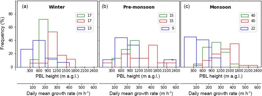
2600 K. Nakoudi et al.: Planetary boundary layer height over New Delhi, India
gradients in the lower parts of the PBL, a higher threshold vations was very satisfying (r = 0.92 and r = 0.95, on 1 and
(0.08) was used in conjunction with cutoff heights (90 m). 2 March).
Furthermore, low aerosol load conditions were responsible
for high variability in the derived PBLH (12:00–14:00 UTC). 4.1.3 Case with low clouds: 29 June 2008
During convective hours (05:00–12:00 UTC), WRF over-
estimated the PBLH mainly due to the simulated neutral In this case broken cumulus clouds appeared between 600
profile-virtual potential temperature at the surface, similar and 1100 m (from 00:00 to 12:00 UTC). On average, a mod-
to that around 1100 m a.g.l. (differences < 0.5 K, not pre- erate PBLH evolution (86 m h−1 ) was found, with a max-
sented), resulting in an increase in the PBLH (Kim et al., imum height (1279 m) appearing at 09:15 UTC (Fig. 5).
2013). It is worth mentioning that, during the convective Whenever clouds appeared below 1 km, we made the as-
period, FMI–PollyXT identified a light aerosol load activ- sumption that the cloud base is an approach to the top of
ity at the altitude at which the numerical model estimated the PBL. However, it could be argued that the PBLH was
the PBLH, with the WCT technique not detecting this activ- at a higher level, where diffuse aerosol layers were found.
ity due to the weakness of the aerosol gradients. At night- In addition, it was difficult to find an adequate signal de-
time, model estimations yielded lower PBLH compared to crease: the default threshold was used, while sensitivity tests
lidar data. The low wind field produced by the WRF close with thresholds sensitive to weaker gradients yielded the
to the surface (wind speed values up to 3 m s−1 in the first same results. Hence, the algorithm exhibited decreased sen-
kilometer) and, thus, the lack of sufficient mechanical turbu- sitivity, which can be attributed to the existence of diffuse
lence, can be related to the shallow nocturnal PBL. It should aerosol layers. High PBLH was observed immediately af-
be noted that the measured PBLH is expected to depict, ter due to a strong aerosol layer which sprawled to lower
apart from any mechanically driven layer during the stable heights, either through dry removal or precipitation that evap-
and transition periods, the top of the previous day’s residual orated before reaching the ground. Following a short rain-
aerosol layer, while the simulated PBLH from WRF refers to fall period (13:30–14:30 UTC), the remaining aerosol kept
the height of the shallow mixed layer. Therefore, their differ- being displaced downwards, creating strong gradients be-
ence is expected since they depict different layers. The over- low 500 m. Moreover, the aerosol removal effect was clear
all correlation was satisfying (r = 0.8). (16:00–24:00 UTC) between 300 and 1000 m. Due to the low
aerosol load, the detection of the PBLH was complicated
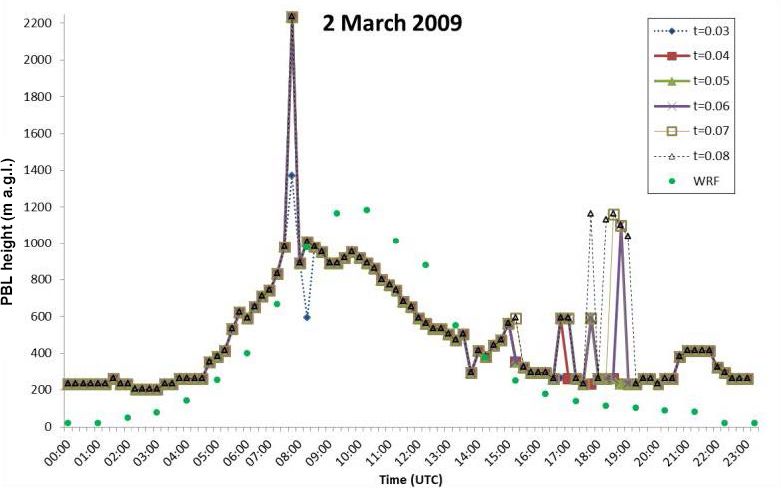
4.1.2 Case with multiple aerosol layers: and, hence, accounted for the high variation in PBLH (16:00–
1–2 March 2009 24:00 UTC). WRF correlated well with FMI–PollyXT (r =
0.74). During the daytime, the WRF slightly overestimated
During the 2-day period of 1–2 March 2009, a complex PBLH, but it should be noted that FMI–PollyXT identified
aerosol layer structure appeared in the free troposphere up to intermittent aerosol gradients at the same altitude, which in-
3 km (Fig. 4). However, appropriate modification of the sig- dicated turbulent activity.
nal decrease threshold and use of appropriate cutoff heights
allowed for the detection of the PBLH. In order to avoid gra- 4.2 Comparison with CALIOP L2 Aerosol Layer
dients in the lower parts of the PBL, the signal threshold was product
adjusted (0.03–0.08) within a 6 %–16 % signal decrease, in
combination with a 30–60 m cutoff zone. During the measurement period, 24 CALIPSO overpasses
On 1 March 2009, the transition period (02:00– were available within 1◦ radius around Gwal Pahari sta-
05:00 UTC) was characterized by a slow PBLH develop- tion. The boundary top location algorithm, SIBYL (selec-
ment (14 m h−1 ), whereas the PBLH evolution was more tive iterated boundary locator), identified two to four lay-
pronounced in the convective period (05:00–09:00 UTC) ers (17 cases), while in the remaining cases no layers were
with a mean growth rate of 101 m h−1 . The maximum identified. However, ground-based lidar observations were
height (950 m) appeared at 08:45 UTC. The next day, a not available in all of the cases (only in 14). Furthermore,
stronger but slightly shorter PBLH cycle was observed, with some cases (5) were excluded from the comparison as the
a mean evolution rate of 187 m h−1 , reaching a maximum detected layers were clearly above the typical PBL limits
height (1010 m) at 08:15 UTC. This slight modification in (higher than 3 km). The comparison of the PBLH between
PBLH development can be attributed to the combination ground-based and space-borne lidar (Fig. 6) was fairly sat-
of higher temperature and lower wind speed conditions on isfying (r = 0.84, statistical significant at 95 % confidence
the second day. On the first day, WRF slightly overesti- level with 0.05 p value), corroborating that the top of the
mated PBLH during the transition period from CBL to RL first detected layer constitutes a good approximation of the
(11:00–14:00 UTC), whereas on the second day an over- PBL top in accordance with relevant studies (Leventidou et
estimation was observed during convective hours (09:00– al., 2013; Korhonen et al., 2014). CALIPSO observations re-
12:00 UTC). During early morning and night, WRF under- vealed slightly higher PBLH, since CALIPSO layer detec-
estimated PBLH, but the overall agreement with lidar obser- tion algorithms in some cases possibly detected aerosol lay-
Atmos. Meas. Tech., 12, 2595–2610, 2019 www.atmos-meas-tech.net/12/2595/2019/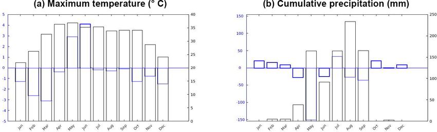
K. Nakoudi et al.: Planetary boundary layer height over New Delhi, India 2601
Figure 3. Evolution of the PBLH observed on 12 February 2009. Range-corrected signal (a) at 1064 nm as measured with FMI–PollyXT .
Black lines indicate 15 min PBLH, while black zones in the lower part of the figure indicate the extent of the signal cutoff area. The color
scale is normalized on a 6 h basis, with red and yellow indicating a higher aerosol load, while green and blue indicate a lower load. PBLH (b)
as given by the FMI–PollyXT and WRF (vertical lines indicate sunrise and sunset times).
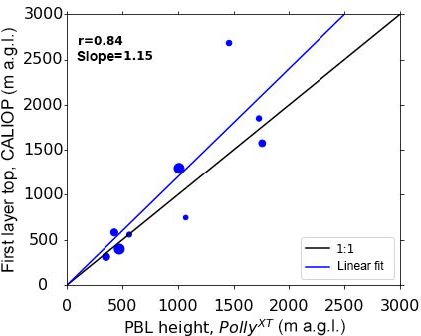
ers, which were transported aloft the PBL. In the majority of nal PBLH is considered here in order to investigate the diur-
the analyzed cases, the detected layers comprised dust lay- nal evolution of the PBLH. In winter, the PBLH cycle as de-
ers with a few cases of dust-polluted dust and dust-polluted fined by FMI–PollyXT reached its maximum (1028 ± 292 m)
smoke mixtures, according to aerosol subtype classification. at 11:00 UTC, while the convective boundary layer height
Based on the analyzed cases, it was found that the over- evolution was completed 2 h earlier (Fig. 7a). In the pre-
pass distance (here 20 and 101 km) from the lidar station and monsoon period, the PBLH growth as derived from lidar
time difference between the measurements did not affect the was completed 3 h prior to PBLH maximization (1249 ±
agreement of the PBLH. Furthermore, the layer top altitude 536 m) (Fig. 7b). In monsoon, FMI–PollyXT revealed a fairly
did not appear to change systematically between daytime and smooth PBLH cycle (Fig. 7c). The maximum PBLH (1192±
nighttime. However, the small number of measurements does 187 m) was observed earlier, compared to winter and the pre-
not allow us to generalize these findings. Hence, longer mea- monsoon season, with high PBLH persisting for a couple of
surement periods or a more extended comparison to ground hours afterwards. Turbulence produced by convection usu-
stations is needed in order to draw more robust conclusions. ally reaches maximum values immediately after the solar
noon, but further growth of the PBLH cannot be sustained
4.3 Statistical analysis for a long period. Nevertheless, PBL did not appear to col-
lapse immediately afterwards, probably due to the remaining
4.3.1 Diurnal cycle of PBLH turbulent fluxes.
Although nighttime PBLH is not taken into account for the
statistical analysis of seasonal PBLH (Sect. 4.3.2), noctur-
www.atmos-meas-tech.net/12/2595/2019/ Atmos. Meas. Tech., 12, 2595–2610, 2019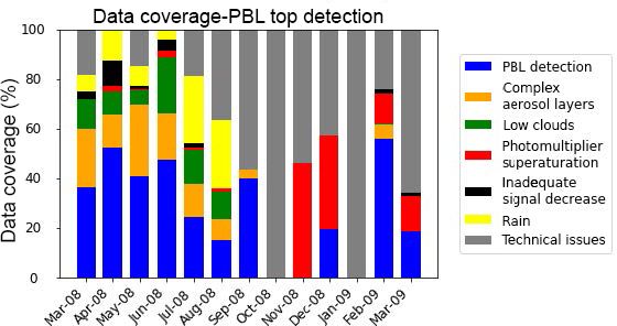
2602                                                K. Nakoudi et al.: Planetary boundary layer height over New Delhi, India

Figure 4. Same as Fig. 3 except for 1–2 March 2009. White horizontal lines (a) indicate 15 min cloud base height.

Figure 5. Same as Fig. 3 except for 29 June 2008. Grey shading (bottom) indicates rainfall.

Atmos. Meas. Tech., 12, 2595–2610, 2019                                                       www.atmos-meas-tech.net/12/2595/2019/
K. Nakoudi et al.: Planetary boundary layer height over New Delhi, India                                                 2603

                                                                 seasonal cycle, with the temperature distribution being simi-
                                                                 lar to the distributions of the whole seasonal periods. During
                                                                 the measuring period, a mean temperature of 21 ± 4 ◦ C was
                                                                 found in winter, 27 ± 3 ◦ C in the pre-monsoon season and
                                                                 30 ± 2 ◦ C in the monsoon season, while the seasonal aver-
                                                                 age maximum temperature was recorded at 29 ± 5, 33 ± 4
                                                                 and 35 ± 2 ◦ C accordingly. Nevertheless, it should be men-
                                                                 tioned that the seasonal cycle of PBLH over Gwal Pahari was
                                                                 weaker than climatologically expected. More specifically,
                                                                 the smoother PBLH cycle could be explained in terms of
                                                                 maximum temperature and cumulative precipitation anoma-
                                                                 lies (Fig. 1). During winter, average maximum temperature
                                                                 was 5 ◦ C higher than the climatological one, while total pre-
                                                                 cipitation was lower (10 mm). On the other hand, during
Figure 6. PBLH comparison for FMI–PollyXT and CALIOP. The        pre-monsoon, the average maximum temperature was lower
heights given by CALIOP have been corrected for elevation. The   by 5 ◦ C than the corresponding climatological record, along
marker size is proportional to the overpass distance from the    with a significantly higher seasonal accumulated precipita-
ground-based lidar.                                              tion (205 mm). The latter is also related to the fact that in
                                                                 2008 (16 June) one of the earliest monsoon onset dates (rain-
                                                                 fall data since 1901) was recorded (Tyagi et al., 2009). Com-
                                                                 pared to another site with similar surroundings and solar cy-
                                                                 cle in Elandsfontein, South Africa, the annual average PBLH
                                                                 was lower in Gwal Pahari (866 m; 1400 m in Elandsfontein)
                                                                 with less seasonal variability (Korhonen et al., 2014).
                                                                    In winter, the daily mean PBLH distribution was narrower
                                                                 (in majority between 600 and 900 m) compared to the pre-
                                                                 monsoon and monsoon seasons (mostly between 900 and
                                                                 1200 m) (Fig. 8). Following a similar pattern, the daily maxi-
                                                                 mum PBLH was rather confined in winter (in majority be-
                                                                 tween 900 and 1200 m) with a significantly broader spec-
                                                                 trum (between 600 and 1800 m) in pre-monsoon and mon-
                                                                 soon seasons. The highest interseasonal variability was ex-
                                                                 hibited during pre-monsoon, which could be attributed to
                                                                 meteorological conditions. The pre-monsoon season com-
                                                                 prised days with heavy rainfall and days with hardly any
                                                                 precipitation, which can potentially explain the broad distri-
Figure 7. PBLH average diurnal cycle in Gwal Pahari according    bution of daily mean PBLH (251–1191 m). In winter large
to FMI–PollyXT during winter (a), pre-monsoon (b) and monsoon    interseasonal variability of maximum PBLH was observed,
seasons (c). Numbers indicate data availability.                 which can be possibly attributed to the broad interseasonal
                                                                 temperature range (20–36 ◦ C).

4.3.2   Daily mean and maximum PBLH                              4.3.3   Daily evolution rate of PBLH

In this section we statistically analyze the seasonal mean       During the measurement period, daily evolution rates
and maximum PBLH cycles as observed from lidar mea-              were mostly within 100–200 m h−1 , but lower rates (29–
surements in conjunction with the seasonal cycle of mean         100 m h−1 ) were observed as well (Fig. 8). In winter, daily
and maximum temperature. The seasonal mean PBLH was              growth rates presented a slightly broad distribution (mostly
found at 695 ± 146 m during winter, 878 ± 297 m during the       between 100 and 200 m h−1 ) with a mean evolution of 157 ±
pre-monsoon period and 1025 ± 296 m during the monsoon.          81 m h−1 (Fig. 8). In the pre-monsoon season, slightly higher
The seasonal average maximum PBLH was determined at              growth rates were observed (mainly within 100–300 m h−1 ),
1191 ± 516 m during winter, 1326 ± 565 m during the pre-         with an average of 206 ± 134 m h−1 . Additionally, rates be-
monsoon period and at 1361 ± 350 m during the monsoon.           tween 0–100 and 500–600 m h−1 were observed, follow-
In general, the PBLH seasonal cycle followed the tempera-        ing the pattern of high interseasonal variability, which was
ture cycle very well. The temperature cycle of the measure-      revealed during the pre-monsoon season (Sect. 4.3.2). In
ment days was fairly representative of the whole 2008–2009       the monsoon, evolution speeds were slightly lower (121 ±

www.atmos-meas-tech.net/12/2595/2019/                                             Atmos. Meas. Tech., 12, 2595–2610, 2019
2604 K. Nakoudi et al.: Planetary boundary layer height over New Delhi, India
Figure 8. Frequency distribution of daily mean (green) PBLH, daily maximum PBLH (red) and daily mean growth rate (blue) as calculated
during the winter period (a), the pre-monsoon season (b) and the monsoon period (c). Numbers indicate data availability.
67 m h−1 ) compared to the pre-monsoon season. The distri- evated layers and PBL internal gradients, which affected the
butions of daily growth rate during pre-monsoon and mon- results when specific thresholds were applied. Higher thresh-
soon show similarities. In order to examine whether the dis- olds appeared to be more sensitive towards detecting lofted
tributions were statistically different we applied the two- layers.
sided Wilcoxon rank sum test (Wilcoxon, 1945; Wilcoxon In the context of the aforementioned cases, the WRF
and Wilcox, 1964). The test yielded that the two distri- model overestimated PBLH in the daytime, while an un-
butions are statistically different at the 95 % significance derestimation was observed at nighttime. The understanding
level. Hence, the differences in the growth rates between of turbulence in nocturnal SBL and its parameterization is
pre-monsoon and monsoon could be possibly related to the rather slow and not well established in numerical weather
weaker diurnal PBLH cycle that was found during the mon- prediction models (Mahrt et al., 1999; Beare et al., 2006;
soon (Fig. 7c). In addition, the different precipitation pat- Hong, 2010). In this study, this is partly addressed by the
terns, with less precipitation during pre-monsoon, could be revised SBL scheme that retains the turbulent levels so as to
attributed to the different growth rates. In Elandsfontein, avoid the abrupt collapse of the mixed layer after the sun-
maximum rates (between 120 and 320 m h−1 ) were reached set by using the exchange coefficients. However, the fact that
during spring, September–October (Korhonen et al., 2014), a neither anthropogenic heat sources nor heat storage in build-
period that exhibits strong similarities with the pre-monsoon ings were included in the simulations could also explain the
season in India. model underestimation. Furthermore, it should be noted that
the measurements often depict different layers from the sim-
ulated ones, as in the case of the residual aerosol layer. De-
5 Summary and conclusions tailed studies of the nocturnal boundary layer, which require
changes in the lidar configuration, such as employment of a
In this study, 1-year-long ground-based lidar measurements near-range and a far-range telescope (Engelmann et al., 2016)
were used to retrieve the PBLH over Gwal Pahari, New can improve the overall consistency in PBLH retrieval ap-
Delhi. The feasibility of deriving the PBLH with the mod- proaches between the model and lidar observations. Satellite
ified WCT technique was investigated and the respective re- lidar observations correlated well with ground-based mea-
sults were compared to independent sources. surements, yielding a higher PBLH due to the detection of
In support of previous work (Baars et al., 2008; Korhonen lofted aerosol layers in some of the cases. These layers can
et al., 2014), it was found that the modified WCT method potentially blanket the PBL and, hence, may strongly attenu-
exhibited satisfying efficiency under different meteorologi- ate the emitted laser beam. More comparisons with ground-
cal and aerosol load regimes. In a case with elevated aerosol based lidar observations are needed to support the finding
layers, significantly good performance was revealed, even that the top of the first layer is indicative of the PBLH.
when the layers were injected into the PBL. Such layers have During the rainy season of the monsoon, the diurnal cycle
been reported in the literature as a major challenge in the at- of PBLH was weaker and its evolution was completed ear-
tribution of the PBLH, especially at nighttime (Haeffelin et lier. A relatively warmer and drier winter and a colder and
al., 2012). PBLH determination was complicated in the pres- rainier pre-monsoon were observed compared to climatolog-
ence of diffuse aerosol layers. A low aerosol load, observed ical records. These meteorological patterns could account for
mainly during morning or afternoon transitions, also repre- the observed PBLH cycle, which was rather indistinct com-
sents a condition for uncertain determination of the PBLH pared to the cycle expected from long-term climate statistics.
(Haeffelin et al., 2012). Sensitivity analysis revealed stable
performance of the WCT algorithm, with the exception of el-
Atmos. Meas. Tech., 12, 2595–2610, 2019 www.atmos-meas-tech.net/12/2595/2019/K. Nakoudi et al.: Planetary boundary layer height over New Delhi, India 2605 Daily evolution rates of 29–200 m h−1 were mainly observed, Data availability. The Gual Pahari lidar data quicklooks and im- with lower rates during the monsoon. ages are available at the PollyNET website (http://polly.tropos.de/, Future studies are necessary in order to better understand last access: 11 April 2019). PollyNET raw data are available on re- the factors that modulate the exchange of moisture, heat and quest from the respective PI. momentum between the surface and PBL and, consequently, affect the comparison of modeled PBLH with observational data. In addition, the relative contribution of the various PBL dynamics drivers, under different aerosol loads and meteorological regimes, needs to be further investigated. The feasibility of applying the modified WCT method in simpler lidar systems such as ceilometer and Doppler lidar should be assessed. These systems entail less operational cost and, thus, exhibit good potential for determining the PBLH and evaluating weather prediction and pollution dispersion models on an operational basis. In recent years, significant effort has been made towards the establishment of ceilometer networks by national weather services and other agencies over Europe with the aim to build up a framework for real-time applications and improvements of air quality and weather prediction by assimilation of ceilometer data (Haeffelin et al., 2012; Wiegner et al., 2014). Analogous efforts are currently in progress over different parts of India, like in the states of Maharashtra and Kerala and in the union territory of Delhi (Sharma et al., 2016; Babu et al., 2017; https://www.lufft.com/projects/ several-lufft-chm-15k-ceilometer-projects-in-india-529/, last access: 11 April 2019). www.atmos-meas-tech.net/12/2595/2019/ Atmos. Meas. Tech., 12, 2595–2610, 2019
2606                                             K. Nakoudi et al.: Planetary boundary layer height over New Delhi, India

Appendix A: Sensitivity analysis of the WCT threshold

In cases of elevated layers or aerosol gradients within the
PBL, it has been revealed that the signal decrease threshold
needs to be properly adjusted (Sect. 4.1). In this study, we
adapted the threshold (t) so that the WCT algorithm was al-
lowed to identify signal gradients on the order of 6 %–16 %
(t = 0.03–0.08). In this section, we investigate the effect of
the WCT threshold on the estimated PBLH. For this reason,
we performed a sensitivity analysis by modifying the signal
decrease threshold for the case of 2 March 2009, when ele-
vated layers were injected into the PBL.
   The overall performance of the WCT technique was sta-
ble (Fig. A1), with the threshold affecting the results in
                                                                  Figure A1. Sensitivity analysis of the WCT method for the case of
only a few cases. When the lowest and more sensitive              2 March 2009. PBLH was estimated by FMI–PollyXT after modifi-
to detect weak layers threshold (0.03) was applied, a thin        cation of the WCT threshold, and by the WRF model.
aerosol layer (around 1300 m) was identified (see Fig. 4).
At this time (07:00 UTC), increased thresholds (0.04–0.08)
detected a stronger elevated layer (approximately at 2 km).       Appendix B: Statistical indicators
The lowest threshold was also more efficient when gra-
dients appeared inside the PBL (around 17:00 UTC), with           Pearson correlation coefficient:
the higher thresholds yielding increased PBLH by approxi-                   N
mately 300 m. When the elevated layers were characterized
                                                                            P                 ¯
                                                                             Oi − Ō · (Mi − M̄)
by a higher aerosol load (18:00–19:00 UTC), lower thresh-         R= s
                                                                         i=1
                                                                                       s              .                       (B1)
olds (0.03–0.05) performed better as well, with the higher             N                 N
                                                                          (Oi − Ō)2 ·     (Mi − M̄)2
                                                                       P                 P
ones identifying stronger layers (around 1 km). Thus, the
                                                                         i=1                i=1
PBLH deviation, introduced by the modification of the WCT
threshold, appeared to depend on the altitude of internal gra-    Mi denotes predicted values from models, while Oi stands
dients or elevated layers. However, in the early morning          for observations at i. N is the number of samples.
(00:00–03:00 UTC), where the convective activity was not
initiated yet, a minor fluctuation (30 m) was observed, re-
lated to the algorithm’s sensitivity towards aerosol content
gradients.
   An adequate threshold adaptation also affected the agree-
ment with the modeled PBLH. More specifically, it is shown
(Fig. A1) that, during cases in which the applied threshold in-
duced a deviation from the smooth PBLH evolution, the dis-
agreement with modeled PBLH increased as well. Besides,
the agreement with the simulated PBLH appeared to depend
on the altitude of the atmospheric features (internal or ele-
vated aerosol gradients) that affected the performance of the
WCT algorithm.

Atmos. Meas. Tech., 12, 2595–2610, 2019                                             www.atmos-meas-tech.net/12/2595/2019/
K. Nakoudi et al.: Planetary boundary layer height over New Delhi, India 2607
Author contributions. KN wrote the manuscript, processed and an- Raman-polarization lidars for continuous aerosol profiling, At-
alyzed the lidar data. EG came up with the study approach, method- mos. Chem. Phys., 16, 5111–5137, https://doi.org/10.5194/acp-
ology and performed experiments. MT came up with the numeri- 16-5111-2016, 2016.
cal modelling approach and interpreted the lidar–WRF comparison. Babu, S., Kumar, A., Padmalal, D., Nair, S., Resmi, E. A., Sorcar,
AD set up the WRF model in the New Delhi area and performed N., Raj, S. R., and Rejani, R. P.: Annual Report 2017–2018,
the WRF simulations. MK provided the lidar data. All authors con- ESSO-National Centre for Earth Science Studies, Ministry of
tributed with merit revisions of the manuscript. Earth Sciences, Government of India, New Delhi, India, 2017.
Beare, R. J., Macvean, M. K., Holtslag, A. A. M., Cuxart, J., Esau,
I., Golaz, J. C., Jimenez, M. A., Khairoutdinov, M., Kosovic, B.,
Competing interests. The authors declare that they have no conflict Lewellen, D., Lund, T. S., Lundquist, J. K., McCabe, A., Moene,
of interest. A. F., Noh, Y., Raasch, S., and Sullivan, P.: An intercomparison
of large-eddy simulations of the stable boundary layer, Bound.-
Lay. Meteorol., 118, 247–272, 2006.
Acknowledgements. This work (the campaigns) was partly funded Binietoglou, I., Amodeo, A., D’Amico, G., Giunta, A., Madonna,
by the European Integrated Project on Aerosol Cloud Climate and F., and Pappalardo, G.: Examination of possible synergy between
Air Quality Interactions, EUCAARI. This work was supported by lidar and ceilometer for the monitoring of atmospheric aerosols,
the Cy-Tera Project (NEA YPODOMH/STRATH/0308/31), which Proc. SPIE 8182, Lidar Technologies, Techniques, and Measure-
is co-funded by the European Regional Development Fund and the ments for Atmospheric Remote Sensing VII, SPIE 8182, 818209,
Republic of Cyprus through the Research Promotion Foundation. https://doi.org/10.1117/12.897530, 2011.
Boers, R. and Eloranta, E. W.: Lidar measurements of the atmo-
spheric entrainment zone and the potential temperature jump
across the top of the mixed layer, Bound.-Lay. Meteorol., 34,
Review statement. This paper was edited by Vassilis Amiridis and
357–375, 1986.
reviewed by three anonymous referees.
Bravo-Aranda, J. A., de Arruda Moreira, G., Navas-Guzmán,
F., Granados-Muñoz, M. J., Guerrero-Rascado, J. L., Pozo-
Vázquez, D., Arbizu-Barrena, C., Olmo Reyes, F. J., Mal-
References let, M., and Alados Arboledas, L.: A new methodology for
PBL height estimations based on lidar depolarization mea-
Althausen, D., Engelmann, R., Baars, H., Heese, B., Ansmann, A., surements: analysis and comparison against MWR and WRF
Müller, D., and Komppula, M.: Portable Raman Lidar PollyXT model-based results, Atmos. Chem. Phys., 17, 6839–6851,
for Automated Profiling of Aerosol Backscatter, Extinction, https://doi.org/10.5194/acp-17-6839-2017, 2017.
and Depolarization, J. Atmos. Ocean. Tech., 26, 2366–2378, Brooks, I. M.: Finding boundary layer top: Application of a wavelet
https://doi.org/10.1175/2009JTECHA1304.1, 2009. covariance transform to lidar backscatter profiles, J. Atmos.
Amiridis, V., Melas, D., Balis, D. S., Papayannis, A., Founda, D., Ocean. Tech., 20, 1092–1105, 2003.
Katragkou, E., Giannakaki, E., Mamouri, R. E., Gerasopoulos, Chen, F. and Dudhia, J.: Coupling an advanced land surface–
E., and Zerefos, C.: Aerosol Lidar observations and model calcu- hydrology model with the Penn State–NCAR MM5 model-
lations of the Planetary Boundary Layer evolution over Greece, ing system. Part I: Model implementation and sensitivity, Mon.
during the March 2006 Total Solar Eclipse, Atmos. Chem. Phys., Weather Rev., 129, 569–585, 2001.
7, 6181–6189, https://doi.org/10.5194/acp-7-6181-2007, 2007. Cimini, D., De Angelis, F., Dupont, J.-C., Pal, S., and Haeffelin,
Ansmann, A., Riebesell, M., and Weitkamp, C.: Measurements of M.: Mixing layer height retrievals by multichannel microwave
aerosol profiles with Raman lidar, Opt. Lett., 15, 746–748, 1990. radiometer observations, Atmos. Meas. Tech., 6, 2941–2951,
Ansmann, A., Wandinger, U., Riebesell, M., Weitkamp, C., and https://doi.org/10.5194/amt-6-2941-2013, 2013.
Michaelis, W.: Independent measurements of extinction and Cohn, S. A. and Angevine, W. M.: Boundary layer height and en-
backscatter profiles in Cirrus clouds by using a combined Raman trainment zone thickness measured by lidars and wind-profiling
elastic-backscatter Lidar, Appl. Optics, 31, 7113–7131, 1992. radars, J. Appl. Meteorol., 39, 1233–1247, 2000.
Baars, H., Ansmann, A., Engelmann, R., and Althausen, D.: Con- Davis, K. J., Gamage, N., Hagelberg, C. R., Kiemle, C., Lenschow,
tinuous monitoring of the boundary-layer top with lidar, Atmos. D. H., and Sullivan, P. P.: An objective method for deriving at-
Chem. Phys., 8, 7281–7296, https://doi.org/10.5194/acp-8-7281- mospheric structure from airborne lidar observations, J. Atmos.
2008, 2008. Ocean. Tech., 17, 1455–1468, 2000.
Baars, H., Kanitz, T., Engelmann, R., Althausen, D., Heese, de Arruda Moreira, G., Guerrero-Rascado, J. L., Benavent-Oltra, J.
B., Komppula, M., Preißler, J., Tesche, M., Ansmann, A., A., Ortiz-Amezcua, P., Román, R., Esteban Bedoya-Velásquez,
Wandinger, U., Lim, J.-H., Ahn, J. Y., Stachlewska, I. S., A., Bravo-Aranda, J. A., Olmo-Reyes, F. J., Landulfo, E., and
Amiridis, V., Marinou, E., Seifert, P., Hofer, J., Skupin, A., Alados-Arboledas, L.: Analyzing the turbulence in the Planetary
Schneider, F., Bohlmann, S., Foth, A., Bley, S., Pfüller, A., Gian- Boundary Layer by the synergic use of remote sensing systems:
nakaki, E., Lihavainen, H., Viisanen, Y., Hooda, R. K., Pereira, Doppler wind lidar and aerosol elastic lidar, Atmos. Environ.,
S. N., Bortoli, D., Wagner, F., Mattis, I., Janicka, L., Markowicz, 213, 185–195, 2018.
K. M., Achtert, P., Artaxo, P., Pauliquevis, T., Souza, R. A. F., Dionisi, D., Keckhut, P., Liberti, G. L., Cardillo, F., and Con-
Sharma, V. P., van Zyl, P. G., Beukes, J. P., Sun, J., Rohwer, E. geduti, F.: Midlatitude cirrus classification at Rome Tor Ver-
G., Deng, R., Mamouri, R.-E., and Zamorano, F.: An overview of gata through a multichannel Raman–Mie–Rayleigh lidar, Atmos.
the first decade of PollyNET : an emerging network of automated
www.atmos-meas-tech.net/12/2595/2019/ Atmos. Meas. Tech., 12, 2595–2610, 20192608 K. Nakoudi et al.: Planetary boundary layer height over New Delhi, India Chem. Phys., 13, 11853–11868, https://doi.org/10.5194/acp-13- the WRF Surface Layer Formulation, Mon. Weather Rev., 140, 11853-2013, 2013. 898–918, https://doi.org/10.1175/MWR-D-11-00056.1, 2012. Dudhia, J.: Numerical Study of Convection Observed during Jordan, N. S., Hoff, R. M., and Bacmeister, J. T.: Validation of the Winter Monsoon Experiment Using a Mesoscale Two- Goddard Earth Observing System-version 5 MERRA plane- Dimensional Model, J. Atmos. Sci., 46, 3077–3107, 1989. tary boundary layer heights using CALIPSO: VALIDATION Emeis, S., Munkel, C., Vogt, S., Müller, W., and Schafer, K.: At- OF GEOS-5 USING CALIPSO, J. Geophys. Res.-Atmos., 115, mospheric boundary-layer structure from simultaneous SODAR, D24218, https://doi.org/10.1029/2009JD013777, 2010. RASS, and ceilometer measurements, Atmos. Environ., 38, 273– Kain, J. S. and Fritsch, J. M.: A one-dimensional entraining/ de- 286, 2004. training plume model and its application in convective parame- Engelmann, R., Wandinger, U., Ansmann, A., Müller, D., Zerom- terization, J. Atmos. Sci., 47, 2784–2802, 1990. skis, E., Althausen, D., and Wehner, B.: Lidar observations of Kain, J. S. and Fritsch, J. M.: Convective parameterization for the vertical aerosol flux in the planetary boundary layer, J. At- mesoscale models: The Kain-Fritcsh scheme. The representation mos. Ocean. Tech., 25, 1296–1306, 2008. of cumulus convection in numerical models, edited by: Emanuel, Engelmann, R., Kanitz, T., Baars, H., Heese, B., Althausen, D., K. A. and Raymond, D. J., Amer. Meteor. Soc., 246 p., 1993. Skupin, A., Wandinger, U., Komppula, M., Stachlewska, I. S., Kim, Y., Sartelet, K., Raut, J.-C., and Chazette, P.: Evalu- Amiridis, V., Marinou, E., Mattis, I., Linné, H., and Ansmann, ation of the Weather Research and Forecast/Urban Model A.: The automated multiwavelength Raman polarization and Over Greater Paris, Bound.-Lay. Meteorol., 149, 105–132, water-vapor lidar PollyXT : the neXT generation, Atmos. Meas. https://doi.org/10.1007/s10546-013-9838-6, 2013. Tech., 9, 1767–1784, https://doi.org/10.5194/amt-9-1767-2016, Klett, J. D.: Stable analytical inversion solution for processing lidar 2016. returns, Appl. Optics, 20, 211–220, 1981. Garratt, J. R.: The Atmospheric Boundary Layer, 335 pp., Cam- Klett, J. D.: Lidar inversions with variable backscatter/extinction bridge Atmospheric and Space Science Series, Cambridge Univ. velues, Appl. Optics, 24, 211–220, 1985. Press, Cambridge, 1992. Komppula, M., Mielonen, T., Arola, A., Korhonen, K., Lihavainen, Groß, S., Gasteiger, J., Freudenthaler, V., Wiegner, M., Geiß, A., H., Hyvärinen, A.-P., Baars, H., Engelmann, R., Althausen, Schladitz, A., Toledano, C., Kandler, K., Tesche, M., Ans- D., Ansmann, A., Müller, D., Panwar, T. S., Hooda, R. K., mann, A., and Wiedensohler, A.: Characterization of the plan- Sharma, V. P., Kerminen, V.-M., Lehtinen, K. E. J., and Vi- etary boundary layer during SAMUM-2 by means of lidar mea- isanen, Y.: Technical Note: One year of Raman-lidar measure- surements, Tellus, 63B, 695–705, https://doi.org/10.1111/j.1600- ments in Gual Pahari EUCAARI site close to New Delhi in India 0889.2011.00557.x, 2011. – Seasonal characteristics of the aerosol vertical structure, At- Haeffelin, M., Angelini, F., Morille, Y., Martucci, G., Frey, S., mos. Chem. Phys., 12, 4513–4524, https://doi.org/10.5194/acp- Gobbi, G. P., Lolli, S., O’Dowd, C. D., Sauvage, L., Xueref- 12-4513-2012, 2012. Rémy, I., Wastine, B., and Feist, D. G.: Evaluation of Mixing- Korhonen, K., Giannakaki, E., Mielonen, T., Pfüller, A., Laakso, Height Retrievals from Automatic Profiling Lidars and Ceilome- L., Vakkari, V., Baars, H., Engelmann, R., Beukes, J. P., Van ters in View of Future Integrated Networks in Europe, Bound.- Zyl, P. G., Ramandh, A., Ntsangwane, L., Josipovic, M., Ti- Lay. Meteorol., 143, 49–75, https://doi.org/10.1007/s10546-011- itta, P., Fourie, G., Ngwana, I., Chiloane, K., and Komp- 9643-z, 2012. pula, M.: Atmospheric boundary layer top height in South Hegde, P., Pant, P., Naja, M., Dumka, U. C., and Sagar, R.: Africa: measurements with lidar and radiosonde compared to South Asian dust episode in June 2006: Aerosol observations three atmospheric models, Atmos. Chem. Phys., 14, 4263–4278, in the central Himalayas, Geophys. Res. Lett., 34, L23802, https://doi.org/10.5194/acp-14-4263-2014, 2014. https://doi.org/10.1029/2007GL030692, 2007. Kulmala, M., Asmi, A., Lappalainen, H. K., Baltensperger, U., Hong, S.-Y.: A new stable boundary-layer mixing scheme and its Brenguier, J.-L., Facchini, M. C., Hansson, H.-C., Hov, Ø., impact on the simulated East Asian summermonsoon, Q. J. Roy. O’Dowd, C. D., Pöschl, U., Wiedensohler, A., Boers, R., Meteor. Soc., 136, 1481–1496, 2010. Boucher, O., de Leeuw, G., Denier van der Gon, H. A. C., Fe- Hong, S.-Y. and Kim, S.-W.: Stable boundary layer mixing ichter, J., Krejci, R., Laj, P., Lihavainen, H., Lohmann, U., Mc- in a vertical diffusion scheme, Proc. Ninth Annual WRF Figgans, G., Mentel, T., Pilinis, C., Riipinen, I., Schulz, M., User’s Workshop, Boulder, CO, National Center for Atmo- Stohl, A., Swietlicki, E., Vignati, E., Alves, C., Amann, M., spheric Research, 3.3, available at: http://www.mmm.ucar.edu/ Ammann, M., Arabas, S., Artaxo, P., Baars, H., Beddows, D. wrf/users/workshops/WS2008/abstracts/3-03.pdf (last access: C. S., Bergström, R., Beukes, J. P., Bilde, M., Burkhart, J. F., 11 April 2019), 2008. Canonaco, F., Clegg, S. L., Coe, H., Crumeyrolle, S., D’Anna, Hong, S.-Y., Noh, Y., and Dudhia, J.: A new vertical diffusion pack- B., Decesari, S., Gilardoni, S., Fischer, M., Fjaeraa, A. M., Foun- age with an explicit treatment of entrainment processes, Mon. toukis, C., George, C., Gomes, L., Halloran, P., Hamburger, T., Weather Rev., 134, 2318–2341, 2006. Harrison, R. M., Herrmann, H., Hoffmann, T., Hoose, C., Hu, Hyvärinen, A.-P., Lihavainen, H., Komppula, M., Panwar, T. S., M., Hyvärinen, A., Hõrrak, U., Iinuma, Y., Iversen, T., Josipovic, Sharma, V. P., Hooda, R. K., and Viisanen, Y.: Aerosol mea- M., Kanakidou, M., Kiendler-Scharr, A., Kirkevåg, A., Kiss, G., surements at the Gual Pahari EUCAARI station: preliminary re- Klimont, Z., Kolmonen, P., Komppula, M., Kristjánsson, J.-E., sults from in-situ measurements, Atmos. Chem. Phys., 10, 7241– Laakso, L., Laaksonen, A., Labonnote, L., Lanz, V. A., Lehtinen, 7252, https://doi.org/10.5194/acp-10-7241-2010, 2010. K. E. J., Rizzo, L. V., Makkonen, R., Manninen, H. E., McMeek- Jiménez, P. A., Dudhia, J., González-Rouco, J. F., Navarro, J., Mon- ing, G., Merikanto, J., Minikin, A., Mirme, S., Morgan, W. T., távez, J. P., and García-Bustamante, E.: A Revised Scheme for Nemitz, E., O’Donnell, D., Panwar, T. S., Pawlowska, H., Pet- Atmos. Meas. Tech., 12, 2595–2610, 2019 www.atmos-meas-tech.net/12/2595/2019/
You can also read