S5P TROPOMI NO2 slant column retrieval: method, stability, uncertainties and comparisons with OMI - Atmos. Meas. Tech
←
→
Page content transcription
If your browser does not render page correctly, please read the page content below
Atmos. Meas. Tech., 13, 1315–1335, 2020
https://doi.org/10.5194/amt-13-1315-2020
© Author(s) 2020. This work is distributed under
the Creative Commons Attribution 4.0 License.

S5P TROPOMI NO2 slant column retrieval: method, stability,
uncertainties and comparisons with OMI
Jos van Geffen1 , K. Folkert Boersma1,2 , Henk Eskes1 , Maarten Sneep1 , Mark ter Linden1,3 , Marina Zara1,2 , and
J. Pepijn Veefkind1,4
1 SatelliteObservations Department, Royal Netherlands Meteorological Institute (KNMI), De Bilt, the Netherlands
2 Meteorology  and Air Quality Group, Wageningen University (WUR), Wageningen, the Netherlands
3 Science and Technology Corporation (S[&]T), Delft, the Netherlands
4 Faculty of Civil Engineering and Geosciences, Delft University of Technology (TUDelft), Delft, the Netherlands

Correspondence: Jos van Geffen (geffen@knmi.nl)

Received: 5 December 2019 – Discussion started: 16 December 2019
Revised: 13 February 2020 – Accepted: 17 February 2020 – Published: 23 March 2020

Abstract. The Tropospheric Monitoring Instrument                 rection in OMI–QA4ECV but not in TROPOMI: turning that
(TROPOMI), aboard the Sentinel-5 Precursor (S5P) satel-          correction off means about 5 % higher SCDs. The row-to-
lite, launched on 13 October 2017, provides measurements         row variation in the SCDs of TROPOMI, the “stripe ampli-
of atmospheric trace gases and of cloud and aerosol proper-      tude”, is 2.15 µmol m−2 , while for OMI–QA4ECV it is a fac-
ties at an unprecedented spatial resolution of approximately     tor of ∼ 2 (∼ 5) larger in 2005 (2018); still, a so-called stripe
7 × 3.5 km2 (approx. 5.5 × 3.5 km2 as of 6 August 2019),         correction of this non-physical across-track variation is use-
achieving near-global coverage in 1 d. The retrieval of          ful for TROPOMI data. In short, TROPOMI shows a superior
nitrogen dioxide (NO2 ) concentrations is a three-step pro-      performance compared with OMI–QA4ECV and operates as
cedure: slant column density (SCD) retrieval, separation of      anticipated from instrument specifications.
the SCD in its stratospheric and tropospheric components,           The TROPOMI data used in this study cover 30 April 2018
and conversion of these into vertical column densities. This     up to 31 January 2020.
study focusses on the TROPOMI NO2 SCD retrieval: the
retrieval method used, the stability of the SCDs and the SCD
uncertainties, and a comparison with the Ozone Monitoring
Instrument (OMI) NO2 SCDs.                                       1   Introduction
   The statistical uncertainty, based on the spatial variabil-
ity of the SCDs over a remote Pacific Ocean sector, is           Nitrogen dioxide (NO2 ) and nitrogen oxide (NO) – together
8.63 µmol m−2 for all pixels (9.45 µmol m−2 for clear-sky        usually referred to as nitrogen oxides (NOx ) – enter the at-
pixels), which is very stable over time and some 30 % less       mosphere due to anthropogenic and natural processes.
than the long-term average over OMI–QA4ECV data (since              Over remote regions NO2 is primarily located in the strato-
the pixel size reduction TROPOMI uncertainties are ∼ 8 %         sphere, with concentrations in the range of 33–116 µmol m−2
larger). The SCD uncertainty reported by the differential op-    (2 − 7 × 10¹⁵ molec. cm−2 ) between the tropics and high lat-
tical absorption spectroscopy (DOAS) fit is about 10 % larger    itudes. Stratospheric NO2 is involved in photochemical reac-
than the statistical uncertainty, while for OMI–QA4ECV the       tions with ozone and thus may affect the ozone layer, either
DOAS uncertainty is some 20 % larger than its statistical un-    by acting as a catalyst for ozone destruction (Crutzen, 1970;
certainty. Comparison of the SCDs themselves over the Pa-        Seinfeld and Pandis, 2006; Hendrick et al., 2012) or by sup-
cific Ocean, averaged over 1 month, shows that TROPOMI           pressing ozone depletion (Murphy et al., 1993).
is about 5 % higher than OMI–QA4ECV, which seems to be              Tropospheric NO2 plays a key role in air quality issues,
due mainly to the use of the so-called intensity offset cor-     as it directly affects human health (WHO, 2003), with con-
                                                                 centrations of up to 500 µmol m−2 (30 × 1015 molec. cm−2 )

Published by Copernicus Publications on behalf of the European Geosciences Union.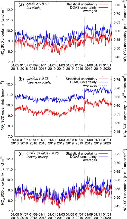
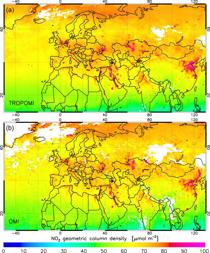
1316                                                        J. van Geffen et al.: S5P/TROPOMI NO2 slant column retrieval

over polluted areas. In addition, nitrogen oxides are essen-
tial precursors for the formation of ozone in the troposphere
(Sillman et al., 1990) and they influence concentrations of
OH and thereby shorten the lifetime of methane (Fuglestvedt
et al., 1999). NO2 in itself is a minor greenhouse gas, but the
indirect effects of NO2 on global climate change are probably
larger, with a presumed net cooling effect mostly driven by
oxidation-fuelled aerosol formation (Shindell et al., 2009).
   The important role of NO2 in both the troposphere and
stratosphere requires monitoring of its concentration on a
global scale, where observations from satellite instruments
provide global coverage, complementary to sparse measure-
ments by ground-based in situ and remote-sensing instru-
ments and measurements with balloons and aircraft. With
lifetimes in the troposphere of only a few hours, the NO2
stays relatively close to its source, and the observations may
be used for top–down emission estimates (Schaub et al.,
2007; Beirle et al., 2011; Wang et al., 2012; van der A et
al., 2017).
   The Tropospheric Monitoring Instrument (TROPOMI;
Veefkind et al., 2012), aboard the European Space Agency
(ESA) Sentinel-5 Precursor (S5P) satellite, which was
launched on 13 October 2017, provides measurements of at-
mospheric trace gases (such as NO2 , O3 , SO2 , HCHO, CH4 ,
CO) and of cloud and aerosol properties at an unprecedented
spatial resolution of 7.2 km (5.6 km as of 6 August 2019)         Figure 1. NO2 geometric column density (GCD, defined in Sect. 4)
along-track by 3.6 km across-track at nadir, with a 2600 km       from TROPOMI (a) and OMI–QA4ECV (b) averaged over 20–
wide swath, thus achieving near-global coverage in 1 d.           26 July 2019 on a common longitude × latitude grid of 0.8◦ × 0.4◦ .
   The TROPOMI NO2 retrieval (van Geffen et al., 2019;            Only clear-sky ground pixels (i.e. with cloud radiance fraction <
Eskes et al., 2020) uses the three-step approach introduced       0.5) are used. The OMI data are filtered for the row anomaly
for the Ozone Monitoring Instrument (OMI) NO2 retrieval           (Sect. 2.2.2).
(the DOMINO approach; Boersma et al., 2007, 2011). This
approach is also applied in the QA4ECV project (Boersma
et al., 2018), which provides a consistent reprocessing for       in this study cover the period 30 April 2018 (which is the start
the NO2 retrieval from measurement by OMI aboard EOS-             of the operational (E2) phase) up to 31 January 2020.
Aura (Levelt et al., 2006, 2018), GOME-2 aboard MetOp-A              OMI NO2 slant column data from QA4ECV (Boersma et
(Munro et al., 2006, 2016), SCIAMACHY aboard Envisat              al., 2018) can be used for comparisons (Sect. 4) because OMI
(Bovensmann et al., 1999), and GOME aboard ERS-2 (Bur-            and TROPOMI provide observations at almost the same lo-
rows et al., 1999).                                               cal time. The example in Fig. 1 shows that both instruments
   The first step is an NO2 slant column density (SCD) re-        capture the larger NO2 hotspots equally well but that OMI
trieval using a differential optical absorption spectroscopy      misses some smaller hotspots and that its measurements are
(DOAS) technique, which provides the total amount of NO2          noisier than TROPOMI’s because the latter has a higher spa-
along the effective light path from sun through atmosphere to     tial resolution and a better signal-to-noise ratio.
satellite. Next, NO2 vertical profile information from a chem-       TROPOMI level-2 data are reported in SI units, which
istry transport model and data assimilation (CTM/DA) sys-         for NO2 means in mol m−2 . For convenience of the reader
tem that assimilates the satellite observations is used to sep-   this paper uses the SI units and in most instances also
arate the stratospheric and tropospheric components of the        provides numbers in the more commonly used unit of
total SCD. And finally these SCD components are converted         molec. cm−2 ; the conversion factor between the two is
to NO2 vertical stratospheric and tropospheric column den-        6.02214 × 10¹⁹ mol−1 .
sities using appropriate air-mass factors (AMFs).
   This paper focusses on the first step, the TROPOMI NO2
SCD retrieval: it provides details of the retrieval method
(Sect. 3), analyses the stability and uncertainties of the SCD
retrieval (Sect. 4), and discusses some further issues related
to the NO2 SCD retrieval (Sect. 5). The TROPOMI data used

Atmos. Meas. Tech., 13, 1315–1335, 2020                                              www.atmos-meas-tech.net/13/1315/2020/
J. van Geffen et al.: S5P/TROPOMI NO2 slant column retrieval                                                                   1317

2     Satellite data sources and data selection                     Eichmann, 2019) for use of the data and the data product
                                                                    versions.
2.1     TROPOMI aboard Sentinel-5 Precursor                            To investigate the stability and uncertainties of the
                                                                    TROPOMI NO2 SCDs, orbits over the Pacific Ocean,
2.1.1    TROPOMI instrument                                         i.e. away from anthropogenic sources of NO2 , are used: for
                                                                    each day the first available orbit with satellite (nadir-viewing)
                                                                    Equator crossings west of about −135 ◦ . Such an orbit is
TROPOMI (Veefkind et al., 2012) is a nadir-viewing spec-
                                                                    missing on a few days and these days are thus skipped.
trometer aboard ESA’s S5P spacecraft, which was launched
                                                                       The TROPOMI data used in this study cover the period
in October 2017. From an ascending sun-synchronous po-
                                                                    30 April 2018 (which is the start of the operational (E2)
lar orbit, with an Equator crossing at about 13:30 local time,
                                                                    phase) up to 31 January 2020. Offline (re)processed data of
TROPOMI provides measurements in four channels (UV,
                                                                    versions 1.2.x and 1.3.x are used; these versions do not dif-
visible, NIR and SWIR) of various trace gas concentrations,
                                                                    fer in the SCD retrieval part of the processing and are based
as well as cloud and aerosol properties. In the visible chan-
                                                                    on level-1b version 1.0.0 spectra (Babić et al., 2017). Near
nel (400–496 nm), used for the NO2 retrieval, the spectral
                                                                    real-time (NRT) data are not considered here; validation of
resolution and sampling are 0.54 and 0.20 nm, with a signal-
                                                                    both the offline and NRT data has shown that results of these
to-noise ratio of around 1500. Radiance measurements are
                                                                    processing chains do not differ significantly (Lambert et al.,
taken along the dayside of the Earth; once every 15 orbits a
                                                                    2019).
small part of the dayside orbit near the North Pole is used to
measure the solar irradiance.
                                                                    2.2     OMI aboard EOS-Aura
   Individual ground pixels are 7.2 km (5.6 km as of 6 Au-
gust 2019), with an integration time of 1.08 s (0.84 s), in
                                                                    2.2.1    OMI instrument
the along-track and 3.6 km in the across-track direction at
the middle of the swath. There are 450 ground pixels (rows)
                                                                    OMI (Levelt et al., 2006) is a nadir-viewing spectrometer
across-track and their size remains more or less constant to-
                                                                    aboard NASA’s EOS-Aura spacecraft, which was launched
wards the edges of the swath (the largest pixels are ∼ 14 km
                                                                    in July 2004. From an ascending sun-synchronous polar or-
wide). The full swath width is about 2600 km and with that
                                                                    bit, with an Equator crossing at about 13:40 local time, OMI
TROPOMI achieves global coverage each day, except for
                                                                    provides measurements in three channels (two UV and one
narrow strips between orbits of about 0.5◦ width at the Equa-
                                                                    visible) of various trace gas concentrations, as well as cloud
tor. Along-track there are 3245 or 3246 scanlines (4172 or
                                                                    and aerosol properties. In the visible channel (349–504 nm),
4173 after the along-track pixel size reduction) in regular ra-
                                                                    used for the NO2 retrieval, the spectral resolution and sam-
diance orbits, leading to about 1.46 (1.88) million ground
                                                                    pling are 0.63 nm and 0.21 nm, with a signal-to-noise ratio
pixels per orbit; for orbits with irradiance measurements
                                                                    of around 500. Radiance measurements are taken along the
there are about 10 % fewer scanlines. Approximately 15 %
                                                                    dayside of the Earth; once every 15 orbits a small part of the
of the ground pixels are not processed due to the limit on the
                                                                    dayside orbit near the North Pole is used to measure the solar
solar zenith angle (θ0 ≤ 88◦ ) in the processing.
                                                                    irradiance.
   Over very bright radiance scenes, such as high clouds,
                                                                       Individual ground pixels are 13 km, with an integration
the CCD detectors containing band 4 (visible; e.g. used for
                                                                    time of 2 s, in the along-track and 24 km in the across-track
NO2 retrieval) and band 6 (NIR; e.g. used for cloud data re-
                                                                    direction at the middle of the swath. There are 60 ground pix-
trieval) may show saturation effects (Ludewig et al., 2020),
                                                                    els (rows) across-track and their size increases towards the
leading to lower-than-expected radiances for certain spec-
                                                                    edges of the swath to ∼ 150 km. The full swath width is about
tral (i.e. wavelength) pixels. In large saturation cases, charge
                                                                    2600 km, and with that OMI achieves global coverage each
blooming may occur: excess charge flows from saturated into
                                                                    day. Along-track there are 1643 or 1644 scanlines in regular
neighbouring detector (ground) pixels in the row direction,
                                                                    radiance orbits, leading to just under 100 000 ground pixels
resulting in higher than expected radiances for certain spec-
                                                                    per orbit; for orbits with irradiance measurements there are
tral pixels. Version 1.0.0 of the level-1b spectra contains flag-
                                                                    about 10 % fewer scanlines.
ging for saturation but not for blooming; version 2.0.0 will
also have flagging for blooming (Ludewig et al., 2020).
                                                                    2.2.2    OMI observations used in this study

2.1.2    TROPOMI observations used in this study                    Comparisons of the magnitude of the NO2 SCDs of
                                                                    TROPOMI and OMI are done using OMI orbits from 2018
The TROPOMI NO2 data retrieval is described in the product          to 2019 as processed within the framework of the QA4ECV
Algorithm Theoretical Basis Document (ATBD; van Geffen              project (Boersma et al., 2018). Since June 2007 a part of the
et al., 2019); see also the Product User Manual (PUM; Eskes         OMI detector has suffered from a so-called row anomaly,
et al., 2019) and the Product ReadMe File (PRF; Eskes and           which appears as a signal suppression in the level-1b radi-

www.atmos-meas-tech.net/13/1315/2020/                                                 Atmos. Meas. Tech., 13, 1315–1335, 2020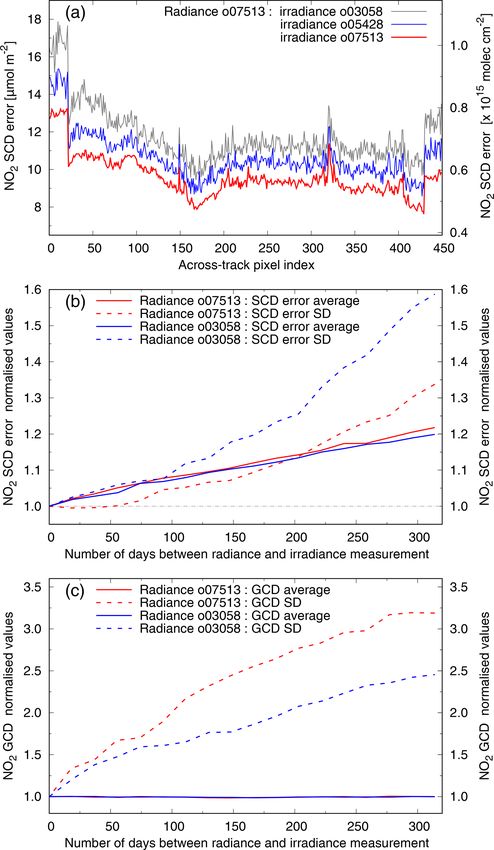
1318                                                           J. van Geffen et al.: S5P/TROPOMI NO2 slant column retrieval

ance data at all wavelengths (Schenkeveld et al., 2017), lead-       satellite instrument:
ing, e.g., to large uncertainties in the NO2 SCDs in the af-                        π I (λ)
fected rows 22–53 (0-based). Comparisons of the NO2 SCD              Rmeas (λ) =             ,                                    (1)
                                                                                   µ0 E0 (λ)
uncertainties (Sect. 4.1) are also made with OMI Pacific
Ocean orbits from 2005–2006, the first year after launch, be-        with I (λ) the radiance at the top of the atmosphere, E0 (λ) the
fore the row anomaly occurred. Note that the OMI degrada-            extraterrestrial solar irradiance measured by the same instru-
tion over the past 15 years is small: the SCD statistical un-        ment and µ0 = cos(θ0 ) the cosine of the solar zenith angle;
certainties and SCD error estimates have increased by about          given that the processing is limited to ground pixels mea-
1 % and 2 % per year, respectively (Zara et al., 2018).              sured at θ0 ≤ 88◦ , the division by µ0 in Eq. (1) will not cause
   TROPOMI and OMI measure at about the same local time              problems. Note that both I and E0 also depend on viewing
(the Equator crossing local time differs by about 10 min) but        geometry, but those arguments are left out for brevity.
since TROPOMI travels at about 830 km and OMI at about                  The modelled reflectance, Rmod (λ), is determined from
715 km altitude, TROPOMI orbits take a little longer than            reference spectra of a number of species known to absorb
OMI’s: when TROPOMI has completed one orbit, OMI has                 in the wavelength window used for the SCD retrieval, as
covered ∼ 1.03 orbits. This means that if a given two or-            well as a correction for scattering and absorption by rota-
bits exactly overlap, then 19 orbits later TROPOMI’s Equa-           tional Raman scattering (RRS), the so-called “Ring effect”
tor crossing longitude lies in between the Equator crossing          (see Grainger and Ring, 1962;   P Chance and Spurr, 1997),
longitudes of two OMI orbits, i.e. a longitudinal mismatch           while a polynomial P (λ) = am λm (m = 0, 1, . . . , np ) is
of about 12.5◦ . The difference in orbit overlap plays a role        used to account for spectrally smooth structures resulting
when comparing results from individual orbits (as done in            from molecular (single and multiple) scattering and absorp-
Sect. 4.1) but is not relevant in the case of gridded averaged       tion, aerosol scattering and absorption, and surface albedo
data being used (as done in Fig. 1 and Sect. 4.4).                   effects.
                                                                        The precise formulation of Rmod (λ) and the method used
2.3    Latitudinal range for uncertainty studies                     to minimise the difference between the modelled and mea-
                                                                     sured reflectance differs slightly between the TROPOMI and
To investigate the stability and uncertainties of the NO2 SCD        OMI retrievals. Details of these DOAS approaches are listed
retrieval the “tropical latitude” (TL hereafter) range is de-        in Table 1. (The difference in the degree of the DOAS poly-
fined as all scanlines that have their sub-satellite latitude        nomial is not relevant: np = 4 and np = 5 give practically the
point – corresponding approximately to the nadir-viewing             same results; for TROPOMI np = 5 is chosen following the
detector rows – within a 30◦ range that moves along with             traditional setting in the OMNO2A processing (cf. Sect. 3.4)
the seasons, in an attempt to filter out seasonality in the NO2      of OMI data.)
columns: on 1 January the TL range covers [−30 ◦ , 0 ◦ ] for
the sub-satellite latitude points, while half a year later it cov-   3.2   TROPOMI intensity fit retrieval
ers [0 , +30 ◦ ]. The TL range is also used for the across-
track “de-striping” of the SCDs discussed in Sect. 4.3. For          In the TROPOMI NO2 processor (van Geffen et al., 2019)
TROPOMI (OMI) data the TL range contains about 475                   Rmod (λ) is formulated in an intensity fit (IF hereafter) ap-
(250) scanlines; after the along-track pixel size reduction in       proach:
TROPOMI there are about 610 scanlines in the TL range.                                     "                     #
                                                                                              Xnk
                                                                     Rmod (λ) = P (λ) · exp −     σk (λ) · Ns ,k
                                                                                                 k=1
3     NO2 slant column retrieval
                                                                                          Iring (λ)
                                                                              · 1 + Cring             ,                           (2)
Though this paper discusses the method and results of the                                  E0 (λ)
TROPOMI NO2 slant column retrieval (Sect. 3.2), it is im-
portant to also discuss the retrieval method used for OMI data       with σk (λ) the absolute cross section and Ns, k the slant col-
within the QA4ECV (Sect. 3.3) and OMNO2A (Sect. 3.4)                 umn amount of molecule k = 1, . . . , nk taken into account
approaches because differences in results (Sect. 4) turn out         in the fit: NO2 , ozone, water vapour, liquid water and the
to be mainly related to retrieval method details.                    O2 −O2 collision complex. The physical model accounts for
                                                                     inelastic Raman scattering of incoming sunlight by N2 and
3.1    DOAS technique                                                O2 molecules that leads to the filling-in of the Fraunhofer
                                                                     lines in the radiance spectrum, i.e. the Ring effect. In Eq. (2),
The NO2 SCD retrieval is performed using a DOAS tech-                Cring is the Ring fit coefficient and Iring (λ)/E0 (λ) the sun-
nique (Platt, 1994; Platt and Stutz, 2008), which provides           normalised synthetic Ring spectrum, with E0 (λ) is the mea-
the amount of NO2 along the effective light path, from sun           sured irradiance. The term between parentheses in Eq. (2)
through atmosphere to satellite. This technique attempts to          describes both the contribution of the direct differential ab-
model the reflectance spectrum Rmeas (λ) observed by the             sorption (i.e. the 1), and the modification of these differential

Atmos. Meas. Tech., 13, 1315–1335, 2020                                                 www.atmos-meas-tech.net/13/1315/2020/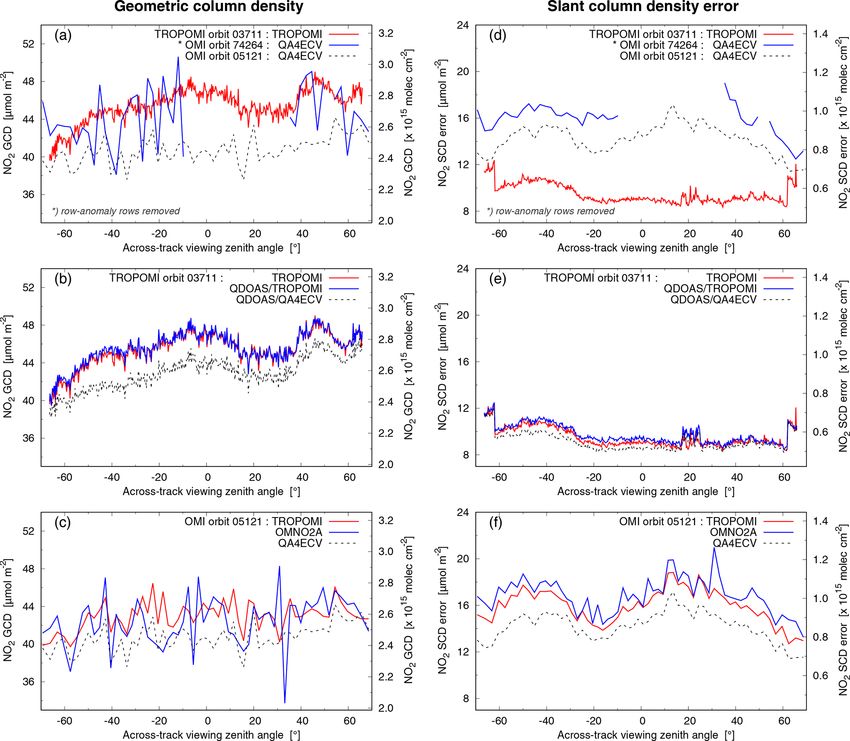
J. van Geffen et al.: S5P/TROPOMI NO2 slant column retrieval                                                                                                               1319

Table 1. Specifics for the NO2 slant column retrieval of TROPOMI and OMI–QA4ECV. The reference spectra (second group of entries) have
all been convolved with the row-dependent instrument spectral response function (ISRF or slit function). Last access dates for all websites
mentioned in the table is 17 March 2020.

                                                TROPOMI                     OMI–QA4ECVa                      Remark, reference or data source
  Type of DOAS fit                              intensity fit                                                van Geffen et al. (2015); van Geffen et al. (2019)
                                                                            optical density fit              Danckaert et al. (2017); Boersma et al. (2018)
  χ 2 minimisation method                       optimal estimation                                           with Gauss–Newton; Rodgers (2000)
                                                                            Levenberg–Marquardt              Press et al. (1997, ch. 15)
  Reference spectrum in Rmeas                   daily E0b                                                    measured once per 15 orbits, i.e. every ∼ 25 h 22 min
                                                                            2005-average E0                  average of OMI irradiance measurements in 2005
  Level-1b uncertainty in χ 2                   included                    not included                     –
  Wavelength range                              405–465 nm                  405–465 nm                       –
  DOAS polynomial degree                        np = 5                      np = 4                           number of coefficients is np + 1
  Intensity offset correction                   not included                constant                         –
  Solar reference spectrum                      Eref                        Eref                             UV–visible channel: Dobber et al. (2008)
  NO2 reference spectrum                        σNO2 at 220 K               σNO2 at 220 K                    Vandaele et al. (1998)
  Ozone reference spectrum                      σO3 at 223 K                σO3 at 243 K                     Serdyuchenko et al. (2014)
  O2 −O2 reference spectrum                     σO2 −O2 at 293 K            σO2 −O2 at 293 K                 Thalman and Volkamer (2013)
  Water vapour reference spectrum               σH2 Ovap at 293 K           σH2 Ovap at 293 K                HITRAN 2012: Rothman et al. (2013)
  Liquid water reference spectrum               σH2 Oliq                    σH2 Oliq                         Pope and Fry (1997)
  Ring reference spectrum                       Iring                       σring                            derived following Chance and Spurr (1997)
  Processor name                                TROPNLL2DP                  QDOAS                            –
  Level-2 offline data version                  v1.2.x & v1.3.x                                              https://s5phub.copernicus.eu/
                                                                            v1.1                             http://www.qa4ecv.eu/
  Level-1b offline data version                 v1.0.0                                                       https://s5phub.copernicus.eu/
                                                                            coll. 3                          https://disc.gsfc.nasa.gov/
a Specifics of the OMI–OMNO2A retrieval are mentioned in Sect. 3.4. b Offline (re)processing uses E measured nearest in time to I , except for the period mid-October 2018 to
                                                                                                   0
mid-March 2019, when the most recent E0 with regard to I was used due to an issue with the processor; the version-2 reprocessing will use the nearest E0 for all orbits.

structures by inelastic scattering (the +Cring Iring (λ)/E0 (λ)                              ground pixels per orbit and thus a significant increase in the
term) to the reflectance spectrum.                                                           number of successfully retrieved ground pixels.
   The IF minimises the chi-squared merit function:                                            The magnitude of χ 2 is a measure of how good the fit is.
                                                                                             Another measure of the goodness of the fit is the so-called
        nλ                           2                                                     root-mean-square (rms) error:
        X    Rmeas (λi ) − Rmod (λi )
χ2 =                                                ,                              (3)              v
                       1Rmeas (λi )
                                                                                                    u
                                                                                                    u1 X   nλ                         2
        i=1
                                                                                             Rrms = t          Rmeas (λi ) − Rmod (λi ) ,               (4)
with nλ the number of wavelengths (spectral pixels) in the fit                                         nλ i=1
window (405–465 nm) and 1Rmeas (λi ) the uncertainty in the
                                                                                             where the difference Rres (λ) = Rmeas (λ)−Rmod (λ) is usually
measured reflectance, which depends on the precision of the
                                                                                             referred to as the residual of the fit.
radiance and irradiance measurements as given in the level-
                                                                                                In the TROPOMI processor χ 2 is minimised using an
1b product, i.e. on the signal-to-noise ratio (SNR) of the mea-
                                                                                             optimal estimation (OE; based on Rodgers, 2000) routine,
surements. Radiance spectral pixels flagged in the level-1b
                                                                                             with suitable a priori values of the fit parameters and a pri-
data as bad or as suffering from saturation (Sect. 2.1.1) are
                                                                                             ori errors set very large, so as not to limit the solution of
filtered out before any further processing step.
                                                                                             the fit (for example, the NO2 SCD a priori error is set at
    In the final data product ground pixels are flagged when
                                                                                             1.0 × 10⁻² mol m−2 = 6 × 10¹⁷ molec. cm−2 ), while for nu-
the slant column retrieval uncertainty 1Ns > 33 µmol m−2
                                                                                             merical stability reasons a pre-whitening of the data is per-
(2 × 10¹⁵ molec. cm−2 ). SCD error values this large occur
                                                                                             formed. Estimated slant column and fitting coefficient uncer-
rarely: usually < 0.1 % of the pixels per orbit with original
                                                                                             tainties are obtained from the diagonal of the covariance ma-
ground pixel sizes; for the smaller-size pixel orbits there are
                                                                                             trix of the standard errors, while the off-diagonal elements
about 50 % more pixels with high SCD error values (based
                                                                                             represent the correlation between the fit parameters.1 The
on one test day of data), taking into account that the SCD
error itself increases with reduced pixel size. Note, however,                                  1 The correlation coefficients, however, are not available in the
that the ground pixel size reduction leads to about 28 % more                                current TROPOMI data product.

www.atmos-meas-tech.net/13/1315/2020/                                                                                Atmos. Meas. Tech., 13, 1315–1335, 2020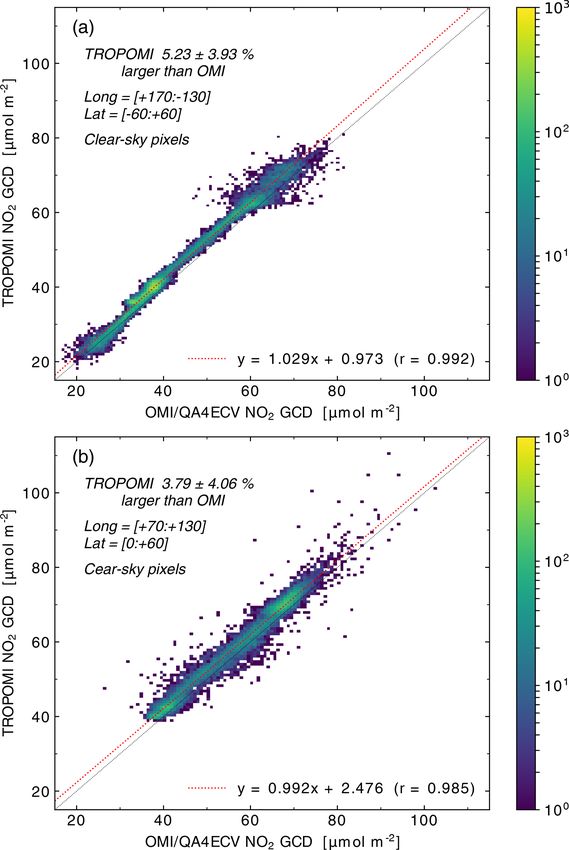
1320                                                         J. van Geffen et al.: S5P/TROPOMI NO2 slant column retrieval

SCD error estimates are scaled with the square root of the
normalised χ 2 , where χ 2 is normalised by (nλ − D), with
D the degrees of freedom of the fit, which isp
                                             almost equal to
the number of fit parameters: 1Ns = 1NsOE · χ 2 /(nλ − D),
with 1NsOE the SCD error reported by the OE routine. The
NO2 output data product provides 1Ns , χ 2 , nλ , D and rms
error.

3.2.1   TROPOMI wavelength calibration

Before forming the reflectance of Eq. (1) both I (λ) and
E0 (λ) are calibrated, after which the calibrated E0 (λcal ) is
interpolated, using information from a high-resolution refer-
ence spectrum (Eref ; see Table 1), to the calibrated I (λcal ),
which serves as the common grid for the reflectance. In the
TROPOMI processor these steps are performed prior to the
DOAS fit (van Geffen et al., 2019).
   A wavelength calibration essentially replaces the nominal
wavelength λnom that comes along with the level-1b spectra
(Ludewig et al., 2020) by a calibrated version:

λcal = λnom + ws + wq (λnom − λ0 ),                         (5)

where ws represents a wavelength shift and wq a wavelength
stretch (wq > 0) or squeeze (wq < 0), with wq defined with         Figure 2. Wavelength calibration shifts ws for the NO2 fit win-
regard to the central wavelength of the fit window λ0 . Each       dow (405–465 nm) of the TROPOMI irradiance (red) and radiance
radiance ground pixel and each irradiance row has its own          (blue), where the latter is an average over the tropical latitude (TL)
wavelength grid and calibration results. In the TROPOMI            range. (a) Shifts for 1 July 2018 (radiance orbit 03711, with irra-
processor fitting wq is turned off; see below for a short dis-     diance from orbit 03718) as a function of the across-track ground
cussion of this.                                                   pixel index; the dashed horizontal lines are the across-track aver-
    The wavelength calibration is performed over the full NO2      ages, with the exception of the outer rows. (b) Time evolution of
fit window (405–465 nm), using a high-resolution solar ref-        the across-track average shifts.
erence spectrum (Eref , pre-convolved with the TROPOMI
instrument spectral response function (ISRF); see Table 1)
and the OE routine also in use for solving the DOAS equa-          rows, 0 and 449, ws shows markedly different values for
tion. For the I (λ) calibration a second-order polynomial as       these rows. To avoid these peaks from overshadowing the
well as a term representing the Ring effect are included: the      effects discussed below, the outer two rows are skipped from
model function used for the radiance wavelength calibration        the following analysis.
is a modified version of Eq. (2); including the Ring effect           The broad across-track shape and the average value of ws
allows for a wavelength calibration to be performed across         visible in Fig. 2a are not important, as they result from the
the full fit window. For the E0 (λ) calibration the Ring term      choice of the nominal grid of the level-1b data. The change
is obviously excluded. The a priori error of the wavelength        in time of the average ws and of the row-to-row variation in
shift is set to 0.07 nm, one-third of the spectral sampling in     ws , however, give an idea of the stability of the level-1b data
the NO2 wavelength range, so as to ensure that ws will not         and hence of the instrument. Figure 2b shows the temporal
exceed the spectral sampling distance.                             change in ws . There seems to be a small long-term oscillation
    Figure 2a shows the wavelength shifts ws for an orbit on       in this, with an amplitude of about 0.0016 and 0.0020 nm for
1 July 2018 of the irradiance (red) and radiance (blue) as a       radiance and irradiance, respectively, which looks likely to
function of across-track ground pixel (row), where the radi-       be a seasonal effect. A similar seasonal variation of similar
ance shift of each row is an along-track average over the TL       amplitude is seen in the wavelength calibration data of OMI’s
range defined in Sect. 2.3. When taking a different latitude       visible channel (Schenkeveld et al., 2017, Fig. 34). Both for
range the across-track shape of the radiance wavelength shift      TROPOMI and OMI this amplitude does not exceed scatter
shown in Fig. 2a does not noticeably change, while the abso-       levels and is thus well within instrument requirements.
lute value of the average shifts increases by about 5 % going         For a given field of view (ground pixel), the dominant term
south to north – it is not known what causes this small in-        in the overall magnitude of the radiance is the inhomoge-
crease, but it is well within instrument specifications. Due       neous illumination of the instrument slit as a result of the
to only partial instrument slit illumination at the outer two      presence of clouds. Variation in the presence of clouds may

Atmos. Meas. Tech., 13, 1315–1335, 2020                                                www.atmos-meas-tech.net/13/1315/2020/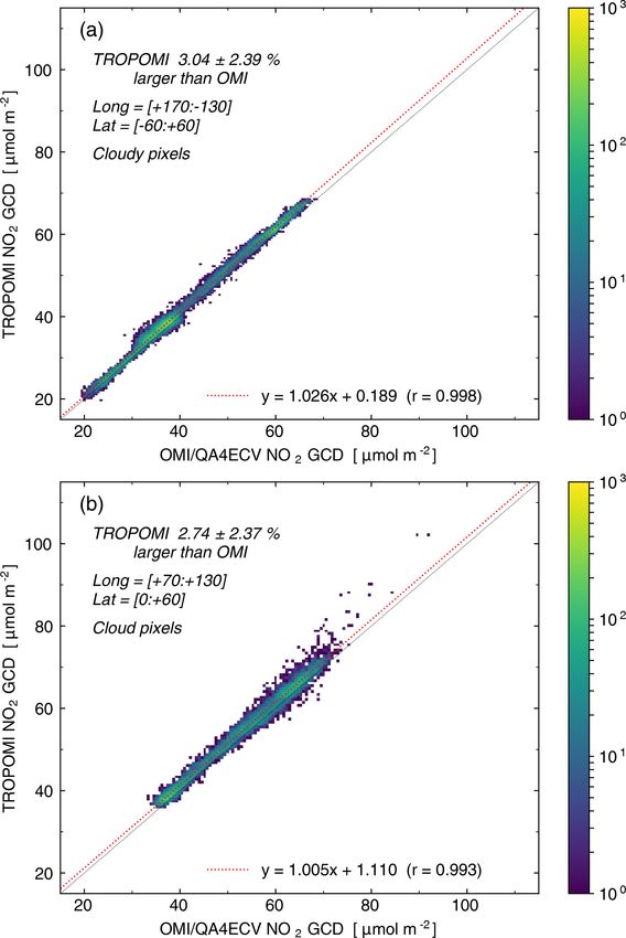
J. van Geffen et al.: S5P/TROPOMI NO2 slant column retrieval                                                                   1321

therefore show up as differences in the ws of ground pixels         without weighting with the level-1b uncertainty estimate
(e.g. along a row) and from day to day. The magnitude of            1Rmeas , though QDOAS has the option to include the
the day-to-day variation in the average is much smaller than        weighting. To minimise χODF  2 , QDOAS uses a Levenberg–

the long-term oscillation visible in Fig. 2b. The row-to-row        Marquardt non-linear least-squares fitting procedure (Press
variation in the shift, visible in Fig. 2a, is small and the evo-   et al., 1997), which also provides an estimate of the uncer-
lution of that across-track variation shows a slow increase         tainties in the fit parameters.
over time (not shown), probably related to degradation of the          In the ODF formulation the rms error is defined as
instrument (Erwin Loots, personal communication, 2019).                       v
                                                                              u       nλ
   With the forthcoming update of the level-1b data to v2.0.0         ODF
                                                                              u1 X                                     2
the nominal UV–visible wavelength grids of both irradiance          Rrms = t               ln Rmeas (λi ) − ln Rmod (λi ) ,  (8)
                                                                                 nλ i=1
and radiance are adjusted by 0.027 nm, for all rows and all
days (Ludewig et al., 2020). As a result of this the average        which is different from the Rrms of the intensity fit as given in
ws will be reduced by that amount, but the across-track and         Eq. (4); see Appendix B for a relationship between the two.
in-time variations will remain the same. Level-1b v2.0.0 will         Like many other DOAS applications, the OMI–QA4ECV
contain an improved degradation correction (Rozemeijer and          processing includes a correction for an intensity offset in the
Kleipool, 2019; Ludewig et al., 2020), probably reducing the        radiance:
slow increase over time of the across-track variation men-
tioned above. All in all, the wavelength calibration results                     π I (λ) + Poff (λ) · Soff
                                                                    Rmeas (λ) =                              ,                    (9)
show that TROPOMI is a rather stable instrument, but fur-                                µ0 E0 (λ)
ther monitoring of the wavelength shifts seems worthwhile.
   Turning on the stretch fit parameter in the radiance calibra-    with Poff (λ) a low-order polynomial (in OMI–QA4ECV a
tion for orbit 03711 leads to a small stretch of 0.2–5 × 10⁻⁴ ,     constant) and Soff a suitable scaling factor (QDOAS com-
depending on latitude, with an associated error estimate of         putes this dynamically from an average of the measured solar
3–6 × 10⁻⁴ (averaging over 30◦ latitude ranges with varying         spectrum E0 (λ) in the DOAS fit window). Sect. 5.1 discusses
central latitudes): the stretch found is smaller than its error     the possible origin and implication of this correction term.
for most latitudes. At the same time the radiance wavelength           QDOAS also has the option to be run in intensity fit mode,
shift, the NO2 SCD and SCD error, and the rms error of the          in which case the modelled reflectance includes the Ring ef-
DOAS fit change on average by less than 1 %, with a stan-           fect as a pseudo-absorber like it does in the optical density fit
dard deviation comparable to that change or larger. In other        mode Eq. (6) rather than as the non-linear term like in Eq. (2).
words: including the stretch fit parameter in the radiance cal-
                                                                    3.3.1    OMI–QA4ECV wavelength calibration
ibration does not significantly alter the retrieval results, and
hence the wq fit parameter will remain turned off.                  In QDOAS (Danckaert et al., 2017) the wavelength calibra-
                                                                    tion of E0 (λ) is performed prior to the DOAS fit, based on a
3.3   OMI–QA4ECV optical density fit retrieval
                                                                    high-resolution solar reference spectrum (Eref ; see Table 1).
The OMI data are processed in the QA4ECV framework                  The calibration of I (λ) is part of the DOAS fit: the shift, ws ,
with the QDOAS software (Danckaert et al., 2017), wherein           and stretch, wq , are fitted along with the SCDs, with the cal-
Rmod (λ) is formulated in an optical density fit (ODF here-         ibrated E0 (λcal ) wavelength grid as the common grid for the
after) approach:                                                    reflectance. For OMI–QA4ECV both a shift and stretch are
                                                                    fitted (cf. Eq. 5) with the stretch negligibly small. When pro-
                   nk
                     X                                              cessing TROPOMI data with QDOAS, only shifts are fitted,
ln Rmod (λ) = P (λ)−    σk (λ)·Ns, k − σring (λ)·Cring , (6)        as is the case for the regular TROPOMI processing.
                         k=1                                            Processing the TROPOMI orbit for which the wavelength
                                                                    shifts are shown in Fig. 2a with QDOAS leads to almost
with σring (λ) the differential (pseudo-absorption) reference
                                                                    identical wavelength shifts: the irradiance and TL average
spectrum of the Ring effect and Cring its fitting coefficient,
                                                                    radiance shifts differ by 0.25 ± 0.10 × 10⁻³ nm and 0.65 ±
where σring (λ) equals Iring (λ)/Eref (λ) minus a second-order
                                                                    0.08 × 10⁻³ nm, respectively (the TROPOMI spectral sam-
polynomial, with Eref a (constant) solar reference spectrum
                                                                    pling is 0.20 nm; Sect. 2.1.1). Consequently, the difference
(which is different from the measured solar spectrum E0 (λ)
                                                                    in radiance wavelength calibration between TROPOMI and
used in Eq. 2). Note that except for the way the Ring effect is
                                                                    QDOAS will not affect comparisons of the retrieval results
treated, the IF and ODF modelled reflectances are the same to
                                                                    noticeably.
first order; see Appendix A for a discussion of this difference.
   The ODF minimises the merit function (cf. Eq. 3):                3.4     OMI–OMNO2A intensity fit retrieval
         nλ                                  2                   The official OMI NO2 SCD data processing, running at
         X
 2

χODF =          ln Rmeas (λi ) − ln Rmod (λi ) ,             (7)
         i=1                                                        NASA, is called OMNO2A. OMNO2A v1.2.x delivers

www.atmos-meas-tech.net/13/1315/2020/                                                 Atmos. Meas. Tech., 13, 1315–1335, 2020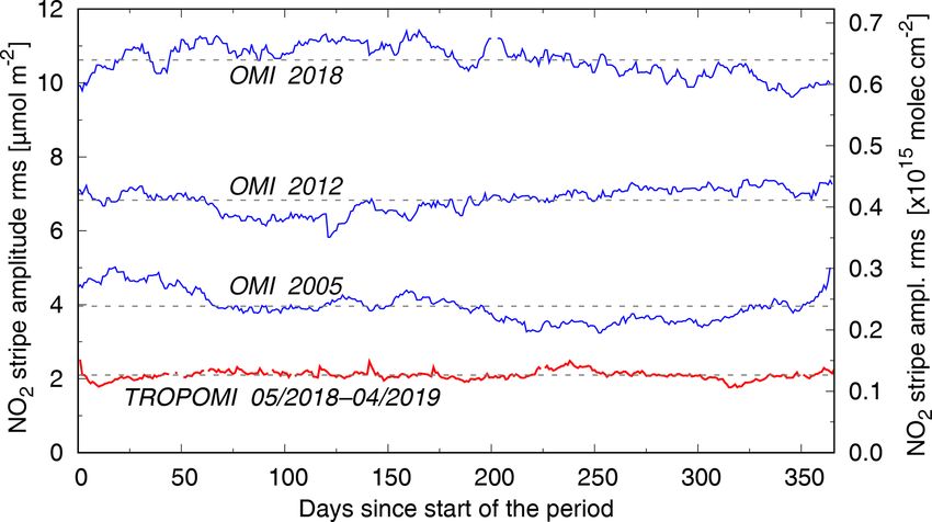
1322                                                        J. van Geffen et al.: S5P/TROPOMI NO2 slant column retrieval

the SCD data for the DOMINO v2 NO2 vertical column                shown in subsequent sections by the stability of stripe ampli-
density (VCD) processing (results of which are released           tude (Sect. 4.3) and slant column uncertainties (Sect. 4.6).
via http://www.temis.nl/airpollution/no2.html, last access:
17 March 2020). A number of improvements intended for
                                                                  4.1.1   Geometric column density
OMNO2A v2.0, which have not yet been implemented, were
investigated by van Geffen et al. (2015), but the SCD retrieval
of OMNO2A v2.0 can be run locally at the Royal Nether-            In Fig. 3a the GCD results of the regular TROPOMI process-
lands Meteorological Institute (KNMI) for testing and com-        ing are compared with the OMI–QA4ECV processing. The
parisons. The OMNO2A processor does not include an in-            TROPOMI and OMI GCD of 1 July 2018 compare well in
tensity offset correction term.                                   magnitude, in as far as such a comparison is possible in view
   OMNO2A v2.0 uses the intensity fit approach with the           of the large row-to-row variation in the OMI data and the row
modelled reflectance formulated in the same manner as             anomaly: averaged over the viewing zenith angle range θ =
TROPOMI, viz. Eq. (2) and the settings listed for TROPOMI         [−55◦ , −10◦ ] TROPOMI’s GCD is about 3 % higher than
in Table 1, with the exception that χ 2 is minimised using        OMI’s. Near the western (left) edge of the swath, TROPOMI
a Levenberg–Marquardt (LM) solver and wavelength cali-            seems to report lower NO2 values than OMI, which might
bration is performed over part of the NO2 fit window (409–        be related to the fact that nadir of the OMI orbit lies 9◦ east
428 nm), the 2005 average irradiance spectrum as reference        of TROPOMI nadir. The OMI GCD of 1 July 2005 clearly
and an older ozone reference spectrum (van Geffen et al.,         shows less row-to-row variation than the OMI 2018 data but
2015). Tests have shown that the LM and OE solvers es-            more than the TROPOMI data (cf. Sect. 4.3).
sentially give the same fit results when used with the same          In Fig. 3b the regular TROPOMI results are compared with
settings. Furthermore, KNMI has a local tool to convert the       a processing of the TROPOMI level-1b data with QDOAS,
OMI level-1b data into the TROPOMI level-1b format, en-           using settings as close as possible to those of the TROPOMI
abling direct comparisons between the two processors.             processor and settings used for QA4ECV (viz. Table 1).
                                                                  When using TROPOMI settings the QDOAS results match
                                                                  those of the regular TROPOMI processing very closely: av-
                                                                  eraged over the central 150 (of the 450) detector rows the
4     NO2 slant column retrieval evaluation                       difference is about 0.2 %. The QDOAS QA4ECV settings are
                                                                  different from the TROPOMI settings at three points (type of
This section discusses the NO2 SCD retrieval results of se-       DOAS fit, use of level-1b uncertainly in χ 2 minimisation and
lected TROPOMI orbits in comparison with OMI orbits and           intensity offset correction), as a result of which the GCDs
additional retrieval results using QDOAS (Danckaert et al.        (and thus the SCDs) are lower by about 6.1 % for this orbit.
(2017); version r1771, dated 20 March 2018, is used here).        Sect. 4.2 discusses the effect of the QDOAS settings some-
   The SCD depends strongly on the along-track and across-        what further.
track variation in solar zenith angle (θ0 ) and viewing zenith       In Fig. 3c the OMI results of the regular QA4ECV pro-
angle (θ ). To make evaluations and comparisons easier, the       cessing are compared with a processing of the OMI level-
SCD is divided by the geometric AMF, defined as Mgeo =            1b data with the OMNO2A and TROPOMI SCD processors
1/ cos(θ0 )+1/ cos(θ ), which is a simple but realistic approx-   for the OMI orbit of 2005 in Fig. 3a, in order to investi-
imation for the air-mass factor for stratospheric NO2 . The       gate the impact of retrieval method details. Differences in
resulting NO2 total column may be called the geometric col-       the results of the OMNO2A and TROPOMI processor are
umn density (GCD), to distinguish it from the total, tropo-       likely mainly due to differences in the wavelength calibra-
spheric and stratospheric VCDs, which are determined using        tion: TROPOMI’s radiance wavelength calibration includes
AMFs based on NO2 profile information coming from the             a correction for the Ring effect, which allows the use of a
CTM/DA model (see Sect. 1).                                       larger calibration window (in this case the NO2 fit window;
                                                                  viz. Sect. 3.2.1), while OMNO2A’s calibration window is
4.1    GCD and SCD error comparison for one orbit                 necessarily limited (viz. Sect. 3.4).
                                                                     As with the TROPOMI data in Fig. 3b, the QA4ECV set-
Figure 3 provides comparisons of the GCD (left column)            tings clearly give the lowest GCD results: averaged over the
and SCD error estimate from the DOAS fit (right column),          central 20 (of the 60) detector rows, the QA4ECV GCD is
averaged over the TL range for the Pacific Ocean orbits of        lower than the OMNO2A processor GCD by about 3.7 % and
TROPOMI and OMI on 1 July 2018. In view of the OMI                lower than the TROPOMI processor GCD by about 7.0 %.
row anomaly, the corresponding OMI orbit of 1 July 2005 is        Note that the across-track striping in the OMI results differs
shown as well, noting that the NO2 concentrations in 2005         markedly between the different processor results, which is
are likely to be different from those in 2018.                    related to a combination of processor differences and the re-
   The TROPOMI orbit used here is representative of all Pa-       sponse to instrumental issues (OMI striping data quoted in
cific Ocean orbits in across-track shape and variability, as is   Sect. 4.3 is taken from OMI–QA4ECV).

Atmos. Meas. Tech., 13, 1315–1335, 2020                                             www.atmos-meas-tech.net/13/1315/2020/
J. van Geffen et al.: S5P/TROPOMI NO2 slant column retrieval 1323
Figure 3. NO2 geometric column density (GCD, defined in Sect. 4; a, b, c) and slant column density (SCD) error estimate from the DOAS
fit (d, e, f) averaged over the TL range as function of the across-track viewing zenith angle (θ ) of Pacific Ocean orbits of TROPOMI and OMI
on 1 July 2018 and of OMI on 1 July 2005. (a, d) Regular TROPOMI processing of TROPOMI compared with OMI–QA4ECV processing.
(b, e) Regular TROPOMI processing of TROPOMI compared with QDOAS processing with TROPOMI settings and with QA4ECV settings.
(c, f) Regular TROPOMI processing of OMI compared with OMI–QA4ECV and OMNO2A (v2) results.
4.1.2 Slant column density error Figure 3d–f shows that the SCD error estimate for
TROPOMI data is considerably lower than the estimates for
In the case of TROPOMI, on-board across-track binning of OMI–QA4ECV data. Given that the TROPOMI and OMI re-
measurements takes place: for the outer 22 (20) rows at the trievals are performed with different methods, a direct com-
left (right) edge of the swath, the binning factor is 1, while parison between SCD error is only tentative; an indepen-
for the other rows 2 detector pixels are combined, in order to dent method to compare SCD uncertainties is discussed in
keep the across-track ground pixel width more or less con- Sect. 4.6. Averaged over θ = [−55◦ , −10◦ ], i.e. away from
stant. As a result of this, the outer rows have a larger spectral the row anomaly, TROPOMI’s SCD error is about 40 %
uncertainty, which is reflected in a larger SCD error. The in- (30 %) lower than OMI’s 2018 (2005) data.
creased SCD error visible in the TROPOMI data of Fig. 3d, The reason why the OMI SCD error in 2018 is higher
e around θ ≈ +20◦ is related to the presence of saturation than in 2005 (Fig. 3d) is, at least partly, related to the fact
effects above bright clouds along this particular orbit. that in the OMI processing the 1-year average irradiance of
www.atmos-meas-tech.net/13/1315/2020/ Atmos. Meas. Tech., 13, 1315–1335, 20201324 J. van Geffen et al.: S5P/TROPOMI NO2 slant column retrieval
Table 2. NO2 geometric column density (GCD), slant column density (SCD) error and rms error from the DOAS fit averaged over the TL
range and the central 150 detector rows of TROPOMI Pacific orbit 03711 of 1 July 2018 retrieved with QDOAS using different settings. For
comparison, the regular v1.2.2 TROPOMI results (used in this study) and a local reprocessing using the forthcoming v2.1.0 are also listed.
Given the difference in rms error definitions, their values from QDOAS and TROPOMI retrievals cannot be compared directly (Sect. 3.3).
DOAS Int. off. GCD SCD error rms error
Processor case type correction (µmol m−2 ) (µmol m−2 ) (10−4 ) Remark
QDOAS 1 ODF no 45.93 ± 0.99 9.39 ± 0.25 8.10 ± 0.21
2 ODF yes 43.51 ± 0.79 8.57 ± 0.29 7.36 ± 0.24 QA4ECV config.
3 IF no 46.45 ± 1.03 9.31 ± 0.26 8.82 ± 0.21 TROPOMI config.
4 IF yes 44.22 ± 0.85 8.68 ± 0.29 8.10 ± 0.23
TROPOMI a IF no 46.34 ± 0.95 8.93 ± 0.22 2.22 ± 0.35 v1.2.2
b IF no 46.94 ± 1.00 9.18 ± 0.21 2.21 ± 0.35 v2.1.0 a
c IF yes 45.30 ± 0.87 8.65 ± 0.19 2.08 ± 0.35 v2.1.0 a
a With respect to v1.2.2, v2.1.0 entails two small bug fixes and spike removal (Sect. 4.1.3); all QDOAS runs include spike removal.
2005 is used for all retrievals, and the larger the time dif- the NO2 SCD, SCD error and rms error of the fit: on average
ference between radiance and irradiance measurements, the +2 %, −1 % and −6 %, respectively, based on the evaluation
larger the error on the reflectance and thus on the SCD error of 12 test orbits. A reprocessing of all E2 phase data using
is (cf. Sect. 4.5). This issue has been discussed in detail by v2.0.0 level-1b spectra and NO2 v2.1.0 will probably take
Zara et al. (2018). place sometime in 2020–2021.
Figure 3e shows that the TROPOMI SCD error estimate
compares reasonably well with the estimate provided by 4.2 TROPOMI NO2 SCD: different QDOAS options
QDOAS, despite the differences in retrieval methods: av-
eraged over the central 150 detector rows the difference is As mentioned in the previous section (and visible in Fig. 3),
about +4.2 % with TROPOMI settings and about −2.0 % the retrieval results depend on the details of the DOAS NO2
with QA4ECV settings (see also Sect. 4.2). Figure 3f shows SCD retrieval: the type of the DOAS fit (IF or ODF) and
that in the case of OMI data the SCD error is lowest for the the retrieval settings used (in particular whether the intensity
regular QA4ECV retrieval: the TROPOMI processor reports offset correction is included or not).
a 10.2 % higher and the OMNO2A processor a 15.4 % higher Table 2 presents the GCD, SCD error and rms error of
SCD error. the DOAS fit for four combinations of QDOAS settings
when processing TROPOMI orbit 03711, with other config-
4.1.3 Impact of NO2 processor updates to v2.1.0 uration settings as much as possible matching those of the
TROPOMI processor (if included, the intensity offset correc-
An update of the level-2 NO2 SCD data to version 2.1.0 tion polynomial Poff (λ) is a constant), as well as the results
(planned for late 2020;2 van Geffen et al., 2020) entails two from the TROPOMI NO2 processor. Conclusions from these
small bug fixes in the wavelength assignment and better treat- results are as follows:
ment of saturated radiance spectral pixels and of outliers in
the residual (Appendix C). These improvements have a small – Turning on the intensity offset correction in QDOAS
impact on the absolute value of the NO2 SCD, SCD error and has quite a large impact on the results: the GCD goes
rms error of the fit: on average +0.5 %, +2.5 % and −1 %, down by ∼ 5 %, while the SCD error goes down by
respectively, based on a set of test orbits (see also Table 2). ∼ 8%.
These changes are not expected to alter the averages and tem-
poral stability presented in this paper significantly. – That turning on the intensity offset correction in
TROPOMI level-1b version 1.0.0 spectra suffer from a QDOAS leads to a lower rms error is logical, since
small degradation (Rozemeijer and Kleipool, 2019) of 1 %– an extra fit parameter is introduced; it cannot be deter-
2 %, notably in the irradiance. The update of the level-1b mined which part of the reduction in the rms error (by
spectra to version 2.0.0 (planned for late 2020) will include ∼ 9 %) is due to this extra fit parameter and which part
a correction for the degradation, as well as some calibration is due to a physically better fit.
corrections and improved flagging of saturation and bloom-
ing effects in some spectral pixels (Ludewig et al., 2020). – In IF mode QDOAS retrieves slightly larger GCDs (∼
This update will have a small impact on the absolute value of 1 %) and slightly lower SCD errors (∼ 1 %), showing
that the precise fit method itself does not affect the fit
2 An initially planned new version 2.0.0 will not be deployed. results much.
Atmos. Meas. Tech., 13, 1315–1335, 2020 www.atmos-meas-tech.net/13/1315/2020/J. van Geffen et al.: S5P/TROPOMI NO2 slant column retrieval 1325
– The rms error calculation of the TROPOMI IF mode
and the QDOAS ODF mode, given in Eqs. (4) and (8),
respectively, lead to different results; a relation between
these two is given in Appendix B.
– Given that the rms error in the QDOAS IF mode is
∼ 9 % higher than in the QDOAS ODF mode the rms
definitions of these two QDOAS modes may be slightly
different for the two modes and the definition of the
QDOAS IF mode is different from the TROPOMI IF
mode.
As a reference, Table 2 also includes the results of the reg-
ular TROPOMI retrieval of the currently officially avail-
able processor version v1.2.2, as well as the results from
a local reprocessing with the forthcoming v2.1.0 processor
(Sect. 4.1.3). That processor has an experimental option to
also include an intensity offset correction, implemented in
the form of an extra term on the right-hand side of Eq. (2):
Poff (λ) · Soff
Rmod (λ) = P (λ) · exp [. . .] · (. . .) + , (10)
E0 (λ)
with Poff (λ) a low-order polynomial and Soff a suitable scal-
ing factor with the same unit as E0 (λ). Table 2 shows that
including a constant Poff in the TROPOMI retrieval has a
similar effect as in the case of QDOAS: the GCD and the
SCD error decrease by a few percent.
Another small difference in the retrieval methods is that
the TROPOMI NO2 processor uses the level-1b uncertainty
in χ 2 minimisation (cf. Eq. 3) whereas OMI–QA4ECV does
not (cf. Eq. 7). QDOAS has the option to turn the χ 2 weight-
ing on in its ODF mode, the impact of which on the fit results
(not shown) is minimal for the GCD and rms, while the SCD
error seems to be unrealistically much reduced, indicating
that perhaps the error propagation in the ODF mode is not
done entirely correctly. Figure 4. Evaluation of the NO2 SCD stripe amplitude. (a) SCD
All in all, the retrieval method itself (IF or ODF) does not stripe amplitude Nsstr (blue) and Nsstr /Mgeo , i.e. the GCD stripe
seem to have a significant impact, while the intensity offset amplitude (red), for orbit 03711 of 1 July 2018. (b) The measured
correction has quite a large impact on the GCD (and thus (blue) and corrected (red) GCD for the same orbit, averaged over
on the SCD) values. The intensity offset term is further dis- the TL range. (c) Time evolution of the rms of the SCD stripe am-
cussed in Sect. 5.1. plitude.
4.3 De-striping: correcting across-track features
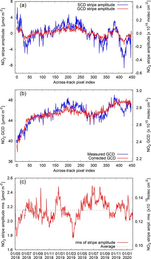
cided to turn on de-striping to remove small but systematic
Since the beginning of the OMI mission, non-physical across-track features and improve the data product quality.
across-track variations in the NO2 SCDs have been observed, The operational TROPOMI de-striping is determined from
which shows up as small row-to-row jumps or “stripes” the TL range of orbits over the Pacific Ocean, and a slant
(Boersma et al., 2011; Veihelmann and Kleipool, 2006). column stripe amplitude is determined for each viewing an-
Given that the geophysical variation in NO2 in the across- gle. The SCD stripe amplitude (Nsstr ) is defined as the differ-
track direction (east–west) is smooth rather than stripe-like ence between the measured total SCD (Ns ) and the total SCD
over non-contaminated areas (Boersma et al., 2007), a proce- (Nscorr = Ns −Nsstr ) derived from the CTM/DA profiles using
dure to “de-stripe” the SCDs is implemented in the CTM/DA the averaging kernel and air-mass factor from the retrieval. In
processing system used for DOMINO and QA4ECV. Even order to retain only features which are slowly varying over
though in TROPOMI the row-to-row variation is much time, and in order to reduce the sensitivity to features ob-
smaller than in OMI (cf. Fig. 3a), as of v1.2.0 it was de- served during a single overpass, the SCD stripe amplitudes
www.atmos-meas-tech.net/13/1315/2020/ Atmos. Meas. Tech., 13, 1315–1335, 20201326 J. van Geffen et al.: S5P/TROPOMI NO2 slant column retrieval
Figure 5. Comparison of the time evolution of the rms of the NO2
SCD stripe amplitude over the first year of TROPOMI data (red;
cf. Fig. 4c) and over selected OMI–QA4ECV years (blue); the main
increases in the OMI rms occur during 2006, 2010–2011 and 2014–
2015. Dashed lines indicate averages over the year periods.
are averaged over a time period of 7 d, or about seven Pacific
orbits, before subtracting them from the SCDs. The NO2 data
product file contains Ns and Nsstr , so that a user of the slant
column data can or must apply the stripe correction.
As an example, Fig. 4a shows Nsstr for the Pacific Ocean
orbit of 1 July 2018 (blue) and Nsstr /Mgeo (red) for the stripe
amplitude in GCD space. For the same orbit Fig. 4b shows
the GCD (blue) averaged over the TL range and the corrected
GCD, i.e. Nscorr /Mgeo (red). The across-track structure and
the magnitude of the Nsstr vary in time, but the overall be-
haviour is fairly constant.
A measure of the stability of the SCD stripe amplitude
is the rms of the across-track
q P stripe amplitude, i.e. of the Figure 6. Comparison of TROPOMI and OMI–QA4ECV NO2
blue line in Fig. 4a: str 2 GCD for clear-sky ground pixels for July 2018 after conversion to
i (Ns, i ) , with summation over
rows i = 0, 1, . . . , 449. Fig. 4c shows this rms as function a common longitude–latitude grid of 0.8◦ × 0.4◦ for (a) the Pacific
of time: there is quite some variation, but on average the Ocean and (b) the India-to-China area. The area covered, the differ-
rms seems constant at 2.15 ± 0.13 µmol m−2 (0.13 ± 0.08 × ence between TROPOMI and OMI–QA4ECV, the linear fit coeffi-
cients, and the correlation coefficient are listed in the panels.
1015 molec. cm−2 ); nothing special is seen at 6 August 2019,
when the pixel size changes. Further monitoring will have to
show whether the stripe amplitude remains stable.
Figure 5 shows the same quantity for the first year 4.4 Quantitative TROPOMI-OMI GCD comparison
of TROPOMI data (average: 2.10 µmol m−2 ) and for se-
lected years of OMI–QA4ECV data: 2005 (3.96 µmol m−2 The comparison of TROPOMI and OMI–QA4ECV Pacific
or 1.9 times the TROPOMI average), 2012 (6.83 µmol m−2 Ocean orbits of 1 July 2018 in Fig. 3a is merely qualitative
or 3.3 times) and 2018 (10.63 µmol m−2 or 5.1 times). because (a) of the row anomaly in the OMI data, (b) of the
The increase in the stripe amplitude of OMI NO2 data stripiness of the OMI data and (c) the orbits do not exactly
is not uniform over time and is also present in the case overlap. For a more quantitative comparison, TROPOMI and
daily solar irradiance spectra being used for the retrieval OMI data are gridded to a common longitude–latitude grid
(Sergey Marchenko, personal communication, 2019); hence of 0.8◦ ×0.4◦ , after applying the respective de-striping of the
the increase is not (or at least not solely) caused by the use SCDs described in the previous subsection on both datasets.
of a fixed irradiance in the OMI–QA4ECV data processing Figure 6 shows the scatter plot of the TROPOMI and
(viz. Table 1), OMI/Q4ERCV GCDs of (almost) clear-sky ground pixels
(i.e. cloud radiance fraction < 0.5) for July 2018 for two re-
gions: the remote Pacific Ocean and the polluted area cover-
ing India and China in the Northern Hemisphere; the def-
inition of these two areas is included in the figure panel
Atmos. Meas. Tech., 13, 1315–1335, 2020 www.atmos-meas-tech.net/13/1315/2020/J. van Geffen et al.: S5P/TROPOMI NO2 slant column retrieval 1327
TROPOMI GCD is on average 1.38 ± 1.26 µmol m−2 or
2.74 ± 2.37 % larger than OMI–QA4ECV.
These differences between the TROPOMI and the OMI–
QA4ECV GCDs (and thus between the SCDs) is comparable
to the difference found in Sect. 4.2 due to turning on the in-
tensity offset correction (discussed further in Sect. 5.1) and
may therefore be related mainly to the specific settings of the
retrieval methods.
4.5 Impact of time difference between radiance and
irradiance measurements
In the offline TROPOMI NO2 (re-)processing of a certain
radiance orbit, the processor is configured to use the irradi-
ance spectrum measured nearest in time to the radiance orbit.
Given that TROPOMI takes irradiance measurements once
every 15 orbits (once every ∼ 25 h and 22 min) and that cur-
rently the offline processing is running at least a week after
the radiance measurements, the difference in time between
the radiance and irradiance measurements will usually be not
larger than eight orbits. In this sense, the TROPOMI pro-
cessing is very different from the OMI processing (whether
QA4ECV, OMNO2A or other): for OMI the 2005 average ir-
radiance is used for the full dataset (2004–present) (van Gef-
fen et al., 2015; Zara et al., 2018).
If for the TROPOMI processor one was to use a fixed irra-
diance, the errors on the retrieval results become larger. Fig-
ure 8a illustrates this by showing the across-track TL range
average SCD error for radiance orbit 07513 using the irradi-
ance measurement of the same orbit and of orbit 05428 (2085
orbits, 147 d earlier) and of orbit 03058 (4455 orbits, 314 d
Figure 7. Same as Fig. 6 but for cloudy ground pixels. earlier): the larger the difference in measurement time be-
tween radiance and irradiance, the larger the SCD error and
the larger the row-to-row variation in the SCD error.
Figure 8b shows the SCD error averaged over detector
legends. Both regions show a very good correlation with rows 25–424 (so as to avoid including the higher uncertain-
R 2 ≈ 0.99. Over the Pacific Ocean area (Fig. 6a) the clear- ties of the outer rows related to the lower on-board pixel
sky TROPOMI GCD is on average 2.20 ± 1.65 µmol m−2 binning) and the corresponding standard deviation (SD) for
(1.33±0.99×10¹⁴ molec. cm−2 ) or 5.23±3.93 % larger than two radiance orbits using selected irradiance measurements
the OMI–QA4ECV GCD. For January 2019 the result (not from between these two; in the case of radiance orbit 03058
shown) is quite similar: the clear-sky TROPOMI GCD over (07513) future (past) irradiances are used. The average SCD
the Pacific Ocean is on average 2.19 ± 1.56 µmol m−2 or error itself increases gradually with increasing time differ-
5.78 ± 4.61 % larger than OMI–QA4ECV. Over the polluted ence, while the SD – a measure of the stripiness of the SCD
India-to-China area (Fig. 6b) the clear-sky TROPOMI GCD error – increases more than linearly with time.
is on average 2.02 ± 2.08 µmol m−2 or 3.79 ± 4.06 % larger For the same series Fig. 8c shows that the average
than OMI–QA4ECV; i.e. the relative difference is a little GCD value itself is not affected by the time difference
smaller than from the Pacific Ocean. between radiance and irradiance: for radiance orbit 03058
For cloudy pixels (i.e. cloud radiance fraction > 0.5) the (07513) the average GCD is 41.11±0.18 µmol m−2 (32.79±
difference between the TROPOMI and OMI–QA4ECV GCD 0.18 µmol m−2 ). The SD of this averaging – the stripiness
is smaller, both in absolute and in relative terms, and the of the GCD – increases steeply, levelling off to a factor of
scatter is less, as can be seen from Fig. 7. Over the Pacific around 3. If the TROPOMI processing were to use a fixed
Ocean area (Fig. 7a) the cloudy TROPOMI GCD is on aver- irradiance, the de-striping (Sect. 4.3) would show an ever in-
age 1.27 ± 0.93 µmol m−2 (0.76 ± 0.56 × 10¹⁴ molec. cm−2 ) creasing stripe amplitude in Fig. 4c.
or 3.04 ± 2.39 % larger than the OMI–QA4ECV GCD. Over It is unclear why the time difference between radiance
the polluted India-to-China area (Fig. 7b) the clear-sky and irradiance measurements has such a big impact on the
www.atmos-meas-tech.net/13/1315/2020/ Atmos. Meas. Tech., 13, 1315–1335, 2020You can also read