Peeking Beneath the Hood of Uber
←
→
Page content transcription
If your browser does not render page correctly, please read the page content below
Peeking Beneath the Hood of Uber

                          Le Chen                                                   Alan Mislove                             Christo Wilson
              Northeastern University                                        Northeastern University                     Northeastern University
                   Boston, MA                                                     Boston, MA                                  Boston, MA
          leonchen@ccs.neu.edu                                           amislove@ccs.neu.edu                             cbw@ccs.neu.edu

ABSTRACT                                                                                        as open platforms, these websites are poised to unlock the
Recently, Uber has emerged as a leader in the “sharing econ-                                    productive potential of millions of people.
omy”. Uber is a “ride sharing” service that matches willing                                        Uber has emerged as a leader in the sharing economy.
drivers with customers looking for rides. However, unlike                                       Uber is a “ride sharing” service that matches willing drivers
other open marketplaces (e.g., AirBnB), Uber is a black-box:                                    (i.e., anyone with a car) with customers looking for rides.
they do not provide data about supply or demand, and prices                                     Uber charges passengers based on time and distance of
are set dynamically by an opaque “surge pricing” algorithm.                                     travel; however, during times of high demand, Uber uses
The lack of transparency has led to concerns about whether                                      a “surge multiplier” to increase prices. Uber provides two
Uber artificially manipulate prices, and whether dynamic                                        justifications for surge pricing [11]: first, it reduces demand
prices are fair to customers and drivers.                                                       by pricing some customers out of the market, thus reducing
   In order to understand the impact of surge pricing on pas-                                   the wait times for the remaining customers. Second, surge
sengers and drivers, we present the first in-depth investiga-                                   pricing increases profits for drivers, thus incentivizing more
tion of Uber. We gathered four weeks of data from Uber by                                       people to drive during times of high demand. Uber’s busi-
emulating 43 copies of the Uber smartphone app and dis-                                         ness model has become so widely emulated that the media
tributing them throughout downtown San Francisco (SF)                                           now refers to the “Uberification” of services [4].
and midtown Manhattan. Using our dataset, we are able to                                           While Uber has become extremely popular, there are also
characterize the dynamics of Uber in SF and Manhattan, as                                       concerns about the fairness, efficacy, and disparate impact
well as identify key implementation details of Uber’s surge                                     of surge pricing. The key difference between Uber and other
price algorithm. Our observations about Uber’s surge price                                      sharing economy marketplaces is that Uber is a black-box:
algorithm raise important questions about the fairness and                                      they do not provide data about supply and demand, and
transparency of this system.                                                                    surge multipliers are set by an opaque algorithm. This lack
                                                                                                of transparency has led to concerns that Uber may arti-
                                                                                                ficially manipulate surge prices to increase profits [25], as
Categories and Subject Descriptors                                                              well as apprehension about the fairness of surge pricing [10].
H.3.5 [Online Information Services]: Commercial ser-                                            These concerns were exacerbated when Uber was forced to
vices, Web-based services                                                                       publicly apologize and refund rides after prices surged dur-
                                                                                                ing Hurricane Sandy [16] and the Sydney hostage crisis [19].
Keywords                                                                                           In order to understand the impact of surge pricing on
                                                                                                passengers and drivers, we present the first in-depth inves-
Uber; Surge Pricing; Sharing Economy; Algorithm Auditing                                        tigation of Uber. We gather four weeks of data from Uber
                                                                                                by emulating 43 copies of the Uber smartphone app and
1.      INTRODUCTION                                                                            distributing them in a grid throughout downtown San Fran-
   Recently, there has been an explosion of services that facil-                                cisco (SF) and midtown Manhattan. By carefully calibrat-
itate the so-called “sharing economy”. Websites like AirBnB,                                    ing the GPS coordinates reported by each emulated app, we
Care.com, TaskRabbit, and Fiverr allow individuals to ad-                                       are able to collect high-fidelity data about surge multipliers,
vertise their services and set their own schedules without the                                  estimated wait times (EWTs), car supply, and passenger
necessity of working for a company. Typically, these web-                                       demand for all types of Ubers (e.g., UberX, UberBLACK,
sites function as marketplaces where participants set their                                     etc.). We validate our methodology using ground-truth data
own prices and choose who to accept jobs from. By acting                                        on New York City (NYC) taxicabs.
                                                                                                   Using our dataset, we are able to characterize the dynam-
Permission to make digital or hard copies of all or part of this work for personal or
classroom use is granted without fee provided that copies are not made or distributed
                                                                                                ics of Uber in SF and Manhattan. As expected, supply and
for profit or commercial advantage and that copies bear this notice and the full citation       demand show daily patterns that peak around rush hours.
on the first page. Copyrights for components of this work owned by others than the              However, we also observe differences between these cities:
author(s) must be honored. Abstracting with credit is permitted. To copy otherwise, or          although SF has many more Ubers than Manhattan, it also
republish, to post on servers or to redistribute to lists, requires prior specific permission   surges much more often. Surge prices are extremely noisy:
and/or a fee. Request permissions from Permissions@acm.org.                                     the majority of surges last less than five minutes. Finally,
IMC’15, October 28–30, 2015, Tokyo, Japan.
Copyright is held by the owner/author(s). Publication rights licensed to ACM.
                                                                                                by analyzing the movements and actions of Uber drivers, we
ACM 978-1-4503-3848-6/15/10 ...$15.00.
DOI: http://dx.doi.org/10.1145/2815675.2815681 .
show that surge prices have a small, positive effect on vehicle
supply, and a large, negative impact on passenger demand.
Additionally, our measured data enables us to identify
key implementation details of Uber’s surge price algorithm.
Based on our understanding of Uber’s algorithm, we make
the following observations:
• Uber has manually divided cities into “surge areas”
with independent surge prices. Prices update every
5 minutes and show high correlation with supply, de-
mand, and estimated wait time over the previous 5-
minute interval. This suggests that surge prices are
set algorithmically, not manually, and that the algo-
rithm is quite responsive.
• However, as April 2015, Uber began serving surge Figure 1: Screenshot of the Uber Partner app.
prices to users that do not always match the prices
returned by the Uber API. Furthermore, surge prices
were no longer uniform for users, even if they were of each trip. Uber retains 20% of each fare and pays the rest
in the same surge area at the same time. We reported to drivers.
this finding to Uber, and their engineers confirmed that Depending on location, Uber offers a variety of different
this behavior was caused by a bug in their system. services. UberX and UberXL are basic sedans and SUVs
• Although we show that surge prices cannot be fore- that compete with traditional taxis, while UberBLACK
cast in advance, given knowledge of the surge pricing and UberSUV are luxury vehicles that compete with
algorithm, we demonstrate how passengers can signif- limousines. UberFAMILY is a subset of UberX and UberXL
icantly reduce surge prices 10-20% of the time by ex- cars equipped with car seats, while UberWAV refers to
ploiting differences between surge areas. wheelchair accessible vehicles. UberT allows users to request
traditional taxis from within the Uber app. UberPOOL al-
Our observations about Uber’s surge price algorithm raise lows passengers to save money via carpooling, i.e., Uber will
important questions about fairness and transparency. For assign multiple passengers to each vehicle. UberRUSH is a
example, users may receive dramatically different prices due delivery service where Uber drivers agree to courier packages
to small changes in geolocation. Furthermore, the vague, on behalf of customers.
changing aspects of the algorithm impacts drivers’ ability Surge Pricing. Uber’s fare calculation changes de-
to predict fares. Finally, the black-box nature of Uber’s pending on local transportation laws. It typically incorpo-
system makes it vulnerable to exploitation by passengers rates a minimum base fare, cost per mile, cost per minute,
(as we show), or possibly by colluding groups of drivers [2]. and fees, tolls, and taxes. The base fare and distance/time
Outline. We begin in §2 by introducing Uber. In §3, charges vary depending on the type of vehicle (e.g., UberX
we present and validate our data collection methodology. vs. UberBLACK).
In §4, we characterize supply and demand on Uber, and In 2012, Uber introduced a dynamic component to pricing
analyze Uber’s surge pricing algorithm in §5. Based on these known as the surge multiplier. As the name suggests, fare
findings, we present a strategy for avoiding surge prices in prices are multiplied by the surge multiplier; typically the
§6, followed by related work and discussion in §7 and §8. multiplier is 1, but during times of high demand it increases.
Uber has stated that there are two goals of this system: first,
2. BACKGROUND higher profits may increase supply by incentivizing drivers
to come online. Second, higher prices may reduce demand
In this section, we briefly introduce Uber, surge pricing,
by discouraging price-elastic customers.
and technical details about the Uber service.
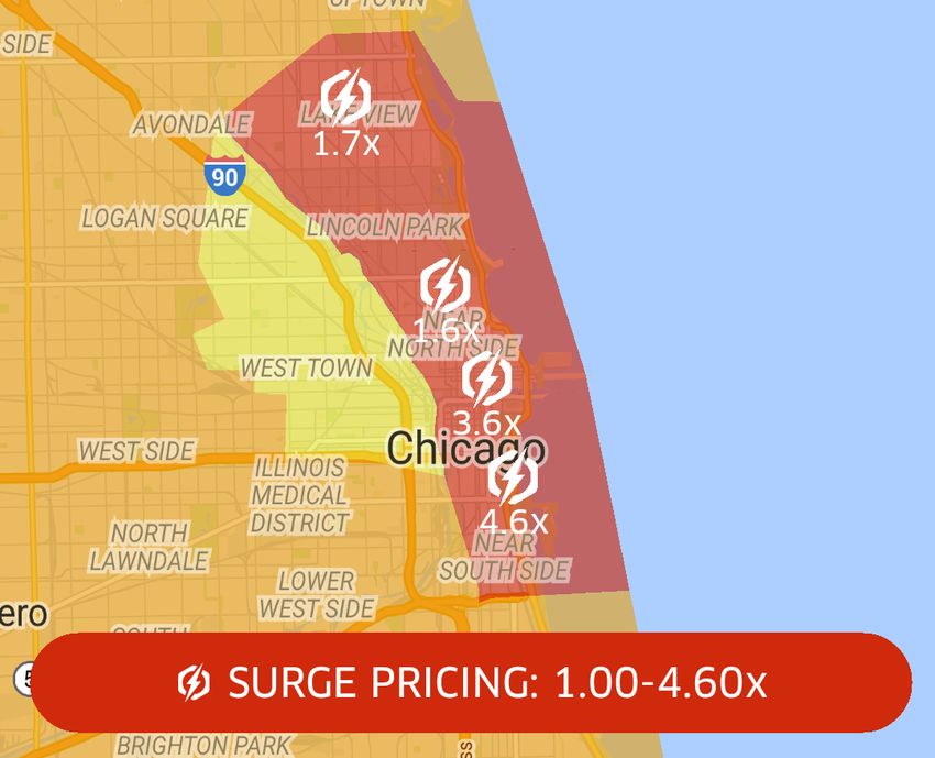
Little is known about Uber’s surge price algorithm, or
Uber. Founded in 2009, Uber is a “ride sharing” ser- whether the system as a whole is successful at addressing
vice that connects people who need transportation with a supply/demand imbalances. As shown in Figure 1, surge
crowd-sourced pool of drivers. Unlike typical transporta- multipliers vary based on location, and recent measurements
tion providers, Uber does not own any vehicles or directly suggest that Uber updates the multipliers every 3-5 min-
hire drivers. Instead, Uber drivers are independent contrac- utes [6]. Uber has a patent pending on the surge price algo-
tors (known as “partners”) who use their own vehicles and rithm, which states that features such as car supply, passen-
set their own schedules. As of May 2015, Uber is available ger demand, weather, and road traffic may be used in the
in 200 cities in 57 countries1 , and claims to have 160K active calculation [23].
drivers in the U.S. alone [15].
Passenger’s Perspective. Uber’s apps provide differ-
Uber provides a platform that connects passengers to
ent information to passengers and drivers. The Client app
drivers in real-time. Drivers use the Uber Partner app
displays a map with the eight closest cars to the user (based
on their smartphone to indicate their willingness to accept
on the smartphone’s geolocation), and the Estimated Wait
fares. Passengers use the Uber Client app to determine the
Time (EWT) for a car. The app provides separate eight-car
availability of rides and get estimated prices. Uber’s system
inventories and EWTs for each type of Uber. Users are not
routes passenger requests to the nearest driver, and auto-
shown the surge multiplier until they attempt to request a
matically charges passengers’ credit cards at the conclusion
car (and only if it is >1). Although the app initially as-
1
https://www.uber.com/cities sumes that the user’s current location is their pickup point,the user may move the map to choose a different pickup for third-party developers to retrieve information about the
point. This new location may have a different EWT and/or state of the service. In our case, the estimates/price and
surge multiplier than the original location. estimates/time endpoints are most useful. The former
Driver’s Perspective. In contrast to the Client takes longitude and latitude as input, and returns a JSON-
app, the Partner app displays very different information to encoded list of price estimates (including surge multipliers)
drivers. As shown in Figure 1, the centerpiece of the Part- for all car types available at the given location. The latter is
ner app is a map with colored polygons indicating areas of similar, except it returns EWTs. Uber imposes a rate limit
surge. Unlike the Client app, the locations of other cars are of 1,000 API requests per hour per user account.
not shown. In theory, this map allows drivers to locate ar- While data from the Uber API is useful, it is not sufficient
eas of high demand where they can earn more money. In for this study, since it does not include information about
practice, drivers often use the Partner and Client apps con- car supply or passenger demand. Thus, we only rely on API
currently, to see the exact locations of competing drivers [3]. data for specific experiments in §5.
The Partner app’s map also suggests that Uber calculates
discreet surge multipliers for different geographic areas. We
empirically derive these surge areas in § 5. 3.3 Collecting Data from the Uber App
To overcome the shortcomings of the Uber API, we lever-
3. METHODOLOGY age the Uber Client app. After a user opens the app and
authenticates with Uber, the app sends pingClient mes-
There are three high-level goals of this study. First, we
sages to Uber’s server every 5 seconds. Each ping includes
aim to understand the overall dynamics of the Uber service.
the user’s geolocation, and the server responds with a JSON-
Second, we want to determine how Uber calculates surge
encoded list of information about all available car types at
multipliers. Third, we want to understand whether surge
the user’s location. For each car type, the nearest eight
pricing is effective at mitigating supply/demand imbalances.
cars, EWT, and surge multiplier are given. Each car is rep-
To answer these questions, we need detailed data about Uber
resented by a unique ID, its current geolocation, and a path
(e.g., supply of cars, surge multipliers, etc.) across time and
vector that traces the recent movements of the car.
geography.
To gather this data, we wrote a script that emulates the
In this section, we discuss our approach for collecting data
exact behavior of the Client app. Our script logs-in to Uber,
from Uber. We begin by motivating San Francisco (SF) and
sends pingClient messages every 5 seconds, and records the
Manhattan as the regions for our study. Next, we discuss our
responses. By controlling the latitude and longitude sent by
methodology for collecting data from the Uber Client app,
the script, we can collect data from arbitrary locations. We
and how we calibrated our measurement apparatus. Finally,
created 43 Uber accounts (each account requires a credit
we validate our methodology using simulations driven by
card to create), giving us the ability to “blanket” a small ge-
ground-truth data on all taxi rides in NYC in 2013.
ographic area with measurement points. To simplify our dis-
3.1 Selecting Locations cussion, we refer to these 43 measurement points as “clients”.
While we were collecting data we never encountered rate
In this study, we focus on the dynamics of Uber in SF limits or had our accounts banned. This indicates that we
and Manhattan. As we discuss in §3.2 and §3.3, there are very likely were not detected by Uber. Although it is possi-
practical issues that force us to constrain our data collection ble that Uber detected our clients and fed them false data, it
to relatively small geographic regions. Furthermore, not all is much more plausible that Uber would have simply banned
regions are viable or interesting: Uber does not offer ser- our clients if they were concerned about our measurements.
vice everywhere, and many places will have few cars and
passengers (i.e., rural areas). Measuring Demand and Supply. Using the data re-
We chose to focus on SF and Manhattan for four rea- turned by pingClient, we can approximate the aggregate
sons. First, San Francisco and New York City have the 2nd supply and demand within our measurement region. To
and 3rd largest populations of Uber drivers in the U.S. (Los measure supply, we can simply count the total number of
Angeles has the largest population) [15]. Second, SF was unique cars observed across all measurement points; each
Uber’s launch city, and recent measurements suggest that it of these cars represents a driver who is looking to provide
accounted for 71% of all “taxi” rides in the city in 2014 (the a ride. To measure demand, we can measure the aggre-
highest percentage of any U.S. city; Uber accounted for 29% gate number of cars that go offline (disappear) between re-
of all rides in NYC during 2014) [27]. Third, SF and NYC sponses; one of the reasons a car may go offline is because
are very different cities in terms of culture and access to pub- it picked up a rider (we discuss other potential reasons, and
lic transportation, which may lead to interesting differences how we handle them, below).
in the dynamics of Uber. Limitations. Although pingClient returns more infor-
Fourth and finally, Manhattan is a useful location to mea- mation than the Uber API, there are still four limitations
sure Uber because there also exists a publicly available that we must address. First, clients only receive information
dataset of all taxi rides in NYC for 2013 [22]. We lever- about the eight closest cars. Thus, to measure the overall
age this data in §3.5 to validate the accuracy of our Uber supply of vehicles in a geographic area, we must position the
measurement methodology. 43 clients such that they completely cover the area. This sit-
uation is further complicated by the fact that each client’s
3.2 The Uber API visibility changes as the density of Uber cars fluctuates (e.g.,
Now that we have chosen locations, the next step is to cars are dense during rush hour but sparse at 4am). In §3.4,
collect data from Uber in these two areas. Like many we perform calibration experiments to determine the appro-
modern web services, Uber provides an HTTP-based API priate distance to space our clients.Second, the demand we are able to estimate from our data Third, we minimized our impact on Uber itself by col-
is fulfilled demand, i.e., the number of cars that pick up pas- lecting just the data we need to perform the study. The
sengers. Uber does not provide public data about quantity overall effect of our measurements was the same as 43 extra
demanded, i.e., the number of passengers that request rides. users running the Uber Client app. Given that Uber claims
The difference between fulfilled and quantity demand is that millions of users worldwide, we believe this is a worthwhile
some passengers may request a ride but not receive one due tradeoff in order to conduct this research.
to supply shortages. Thus, in this study, when we refer to Other Ride-Sharing Services. Although we at-
“demand”, we are talking about fulfilled demand. tempted to collect data from other ride sharing services,
Third, our measurement of demand may overestimate the these efforts were not successful. Lyft implements “prime
true demand because there are three reasons why a car might time” pricing, but this data is only available after a user
disappear between one response and the next: 1) the car requests a ride. Thus, there was no ethical way for us to
drives outside our measurement area, 2) the driver accepts collect this data. Sidecar does not implement surge pric-
a ride request, or 3) the driver goes offline. We can disam- ing; instead, drivers set their own rates based on time and
biguate case 1 since the Client data includes the path vector distance. These additional variables make it difficult to sys-
for each car. Although we cannot disambiguate cases 2 and tematically collect price information.
3, we can still use car disappearances as an upper-bound on
the fulfilled demand within the measurement area.
Fourth, data from the Client app does not allow us to
3.4 Calibration
track individual Uber drivers over time. Although each car is The next step in our methodology is determining the lo-
assigned a unique ID, these IDs are randomized each time a cations for our 43 clients in SF and Manhattan. This step is
car comes online. Unfortunately, there is no way to overcome crucial; on one hand, if we distribute the clients sparsely, we
this limitation, and thus none of our experiments rely on may only observe a subset of cars and thus underestimate
tracking individual drivers. supply and demand (recall that pingClient responses from
Uber only contain the closest eight cars to each client). On
Phantom Cars. Several press articles claim that Uber’s the other hand, if the clients are too close together, the cars
Client app does not display data about actual Uber cars; in- they observe will overlap, and we will fail to observe supply
stead, they claim that the cars are “phantoms” designed to and demand over a sufficiently large geographic area.
give customers the illusion of supply [26]. Uber has publicly To determine the appropriate placement of our 43 clients,
disputed these claims [5,32], explaining that the data shown we conducted a series of experiments between December
in the Client app is as accurate as possible, given practical 2013 and February 2014. In our first experiment, we chose
constraints like the accuracy of smartphone GPS measure- a random location in Manhattan and placed all 43 clients
ments. Furthermore, Uber stated that car locations may be there for one hour. We then repeated this test over several
slightly perturbed to protect drivers’ safety. We have not days with different random locations around Manhattan and
observed any evidence in our data to suggest that the cars SF. The results of these experiments reveal two important
are phantoms; on the contrary, the cars in our data exhibit details about Uber: first, during each test, all 43 clients
all the hallmarks of human activity, such as diurnal activity observed exactly the same vehicles, surge multipliers, and
patterns (see §4). If Uber does present phantom cars, it is EWTs. This strongly suggests that the data received from
likely that they only do so in rural areas with low supply, pingClient is deterministic.
rather than in major cities like Manhattan and SF. Second, when the clients were placed in areas where we
Uber Driver App. As shown in Figure 1, the Driver would not expect to see surge (e.g., residential neighbor-
app also includes useful information (i.e., the surge map). hoods at 4 a.m.), all 43 clients recorded surge multipliers
However, only registered Uber drivers may log in to the of 1 for the entire hour. This strongly suggests that our
Driver app. We attempted to sign-up as an Uber driver, measurement methodology does not induce surges. As we
but unfortunately Uber requires that drivers sign a docu- show in Figure 8, fulfilled demand in midtown Manhattan
ment prohibiting data-collection from the Driver app. We peaks around 100 rides per hour, so 43 clients is a significant
opted not to sign this agreement. Instead, in §5, we recon- enough number that we would expect surge to increase if the
struct the surge map based on data from the Uber API. algorithm took “views” into account.
The goal of our next experiment is to measure the visibility
Ethics. While conducting this study, we were careful to
radius of clients. Intuitively, this is the distance from a client
collect data in an ethical manner. First, we do not collect
to the furthest of the eight cars returned by pingClient.
any personal information about any Uber users or drivers.
We discussed our study with the Chair of our University’s
Institutional Review Board (IRB); she evaluated it as not
being subject to IRB review because we did not collect per- 1000
Visibility Radius (m)
Midtown Manhattan
sonal information or impact any user’s environment. 800 Downtown SF
Second, we minimize our impact on Uber users and 600
drivers. Before we began our data collection, we conducted
an experiment to see if our measurements would impact 400
Uber users by artificially raising the surge price. Fully dis- 200
cussed below, our results strongly suggests that our mea- 0
surements have no impact on the surge multiplier. More- 12am 3am 6am 9am 12pm 3pm 6pm 9pm 12am
over, at no point in this study did we actually request rides Time of the Day
from any Uber driver, and drivers are not able to observe
our measurement clients in the Driver app. Figure 2: Visibility radius of clients in two cities.(a) Uber in downtown SF. (b) Uber in midtown Manhattan. (c) Taxis in midtown Manhattan.
Figure 3: Locations of our Uber and taxi measurement points in SF and Manhattan.
Once we know the visibility radius in SF and Manhattan, the rides back in real-time. Since the taxi data only includes
we can determine the placement of our 43 clients. pickup and dropoff points, the simulator “drives” each taxi
To calculate the visibility radius, we conduct the fol- in a straight-line from point-to-point. We assume that a taxi
lowing experiment. We 1) place 4 clients, denoted as has gone “offline” if it is idle for more than 3 hours (this filter
C = {c1 , c2 , c3 , c4 }, at the same geolocation; 2) each of the only removes 5% of taxi sessions in the data).
clients “walks” 20 meters Northeast, Northwest, Southeast We built an API in our simulator that offers the same
and Southwest (respectively)
T every 5 seconds; 3) the exper- functionality as Uber’s pingClient: it returns the eight clos-
iment halts when | c Vc | = 0, where Vci is the set of cars est taxis to a given geolocation. Just as with Uber, the ID
observed by client ci ; 4) record the distance Dc from each for each taxi is randomized each time it becomes available.
c ∈ C to the starting point. Given this information, we cal- Given this API, we used our methodology from §3.3 and
culate the visibility radius r (consider a 45◦ -45◦ -90◦ triangle §3.4 to measure the supply and demand of taxis over time.
where r is the leg and Dc is the hypotenuse) as: If the measured values from the simulator’s API are similar
to the ground-truth values, we can confidently say that our
1 X Dc X
r= √ ≈ 0.1768 × Dc methodology will also collect accurate data from Uber.
4 c 2 c Calibration. To make our simulation fair, we calibrated
Figure 2 shows the measured radii in meters when the it by using four taxi clients to determine the visibility radius
clients were placed in downtown SF and midtown Manhat- for taxis in midtown NYC (see §3.4). Taxis are much denser
tan. We chose these specific locations because they are the than Ubers in this area, so r = 100 meters is commensu-
“hearts” of these cities, and thus they are likely to have the rately smaller. Figure 3c shows the locations of our 172 taxi
highest densities of Uber cars. As expected, the visibility clients; compared to Uber clients, it takes 300% more taxi
radius changes throughout the day, with the most obvious clients to cover midtown.
difference being night/day in SF. There are also differences Results. Using our taxi clients, we measured the supply
between the cities: the average radius is 247 ± 2.6 meters and demand of taxis in the simulator between April 4–11,
in Manhattan, versus 387 ± 6.8 meters in SF.2 2013. We chose these dates because they correspond to the
In the end, we chose 200 meters as the radius for our same month and week of our Uber measurements (except in
data collection in midtown Manhattan, and 350 meters in 2013 versus 2015, see §4).
downtown SF. These values represent a conscientious trade- As we discuss in §3.3, neither Uber nor our simulator re-
off between obtaining complete coverage of supply/demand turn direct information about demand. Instead, we assume
and covering a large overall geographic area. Figures 3a that cars that 1) disappear from the measured data, and 2)
and 3b depict the exact positions where we placed our clients were not driving near the outer edge of the measurement
in SF and Manhattan.3 polygon were booked by a passenger.4 We refer to these
events as deaths.
3.5 Validation Figure 4 plots the measured and ground-truth taxi supply
Our final step is to validate our measurement method- and demand per 5-minute interval. The two lines are almost
ology. The fundamental challenge is that we do not have indistinguishable since our taxi clients capture 97% of cars
ground-truth information about supply and demand on and 95% of deaths. The results provide strong evidence
Uber; we attempt to mitigate this through careful placement that our measurement methodology captures most of Uber’s
of our clients, but the key challenge is having confidence that supply and demand.
we will observe the vast majority of cars.
To address this issue, we constructed an Uber simula-
tor powered by ground-truth data on NYC taxis [22]. The 4. ANALYSIS
NYC taxi data includes timestamped, geolocated pickup and In this section, we analyze supply, demand, and wait times
dropoff points for all taxi rides in NYC in 2013. Each taxi on Uber. We begin by briefly introducing our datasets and
is assigned a unique ID, so its location can be tracked over how we cleaned them. Next, we examine how the dynamics
time. Our simulator takes the taxi data as input, and plays of Uber change over time and spatially across cities. We
2 4
Throughout this study, we present the 95% confidence in- Restriction (2) is conservative: cars near the edge of the
terval (CI) of the mean value. measurement area may disappear because they were booked,
3
All map images used in this paper are ©2015 Google. or because they drove outside the measurement polygon.3000 1000
(Number of Deaths)
(Number of Cars) Ground Truth Measured Ground Truth Measured
2500 800
2000
Demand
Supply
600
1500
400
1000
500 200
0 0
Apr 04 Apr 05 Apr 06 Apr 07 Apr 08 Apr 09 Apr 10 Apr 11 Apr 04 Apr 05 Apr 06 Apr 07 Apr 08 Apr 09 Apr 10 Apr 11
Days of the Week in Midtown Manhattan, 2013 Days of the Week in Midtown Manhattan, 2013
Figure 4: Measured and ground-truth supply (left) and demand (right) of taxis in midtown Manhattan.
focus the majority of our analysis on UberX, since (as we Client responses by closer vehicles, or the car may only
will show) they are the most common type of Uber by a briefly be near our measurement area. In contrast, cars well-
large margin. We defer detailed analysis of surge multipliers within the boundaries can potentially be observed by many
and the surge pricing algorithm to §5. clients, even as they drive around. Thus, we can safely filter
short-lived cars from our dataset, and focus in the remainder
of the paper only on cars that are driving within the bounds
4.1 Data Collection and Cleaning of our measurement area.
For this study, we collected data from 43 clients placed in
Car Lifespan. Figure 7 shows the lifespans of Ubers
midtown Manhattan and downtown SF between April 3rd–
after removing short-lived cars. We observe similar trends
17th (391 GB of data containing 9.3M samples) and April
in Manhattan and SF: ∼90% of low-priced Ubers (X, XL,
18th–May 2nd (605 GB of data, 9.4M samples), respectively.
FAMILY, and POOL) live forMidtown Manhattan Downtown SF
800
600
Supply
400
200
0
400
UberX UberXL
Demand
300 UberBLACK UberSUV
200
100
0
Surge Multiplier
3.5
3
2.5
2
1.5
1
6
(Minutes)
5
EWT
4
3
2
Apr 04 Apr 05 Apr 06 Apr 07 Apr 08 Apr 09 Apr 10 Apr 11 Apr 18 Apr 19 Apr 20 Apr 21 Apr 22 Apr 23 Apr 24 Apr 25
Timeline Timeline
Figure 8: Supply, demand, surge multiplier, and EWT over time for midtown Manhattan and downtown SF. Surge multiplier
and estimated wait time (EWT) are only shown for UberX. Diurnal patterns are observed in supply and demand, but the
characteristics of the surge multiplier show less predictability.
(a) Avg. Number of Cars (b) Avg. EWT (Minutes) (a) Avg. Number of Cars (b) Avg. EWT (Minutes)
Figure 9: Heatmaps for UberX cars in Manhattan. Figure 10: Heatmaps for UberX cars in SF.
Unsurprisingly, Figure 8 shows that Uber exhibits regular Ubers in Manhattan may be due to greater availability of
daily trends: all four quantities peak during the day and taxis and better public transport. However, Manhattan has
decline at night. We also observe that supply, demand, and more UberXLs, UberBLACKs, and UberSUVs than SF.
EWT have local peaks during morning and afternoon rush Manhattan and SF also exhibit different surge pricing
hour.5 Rush hour peaks are less prominent for surge pricing, characteristics. As shown in Figure 8, downtown SF surges
and we show in §5 that surge pricing is extremely noisy. (i.e., surge >1) more frequently than midtown Manhattan.
Both cities exhibit the same rank ordering of Uber types. Surge multipliers are also tend to be higher in SF: 1.36 ±
UberXs are most prevalent, followed by UberBLACK, Uber- 1 × 10⁻⁴ on average versus 1.07 ± 7 × 10⁻⁵ in Manhattan.
SUV, and UberXL. Both cities also have other types of Ubers In midtown Manhattan, surge tends to increase starting at
(e.g., UberRUSH, UberFAMILY, etc.), however there are 3pm through evening rush hour Monday–Thursday. On the
only 4 cars of these types on the road on average. Manhat- weekends, surge tends to peak between noon and 3pm, likely
tan does have a significant number of UberT’s, but these are due to the influx of tourists. In SF, surge peaks at around
not interesting in our context since they are not subject to 2.0 during morning rush hour (6am–9am) Monday–Friday.
surge pricing (recall that UberT corresponds to an ordinary Surge also has a localized peak at 2am every night (but es-
taxi). Comparing the NYC taxi data in Figure 4 to Figure 8 pecially on weekends, reaching up to 3.0), which is “last call”
we see that there are an order of magnitude more taxis in throughout California.
midtown Manhattan than all Ubers combined. Although Figure 8 focuses on surge multipliers of UberX,
Despite their similarities, Figure 8 also reveals differences other types of Ubers exhibit similar trends. A recent report
between Manhattan and SF. In our measurement region, SF estimated that Uber accounts for 71% of “taxi” rides in SF
has 58% more Ubers overall than Manhattan, mostly due to versus 29% in NYC [27], so it is possible that this difference
the large amount of UberXs in SF. The relative dearth of in demand explains the differences in surge characteristics.
We defer in-depth discussion of surge pricing to §5.
5
Note that the y-axes of supply and demand have different We also observe that Uber offers expedient service in both
scales. cities. Average EWT for an UberX in midtown Manhattan100 100 100
April MHTN
80 80 80 April SF
60 60 60
CDF
CDF
CDF
Feb. MHTN
40 40 40
20 Manhattan 20 Manhattan 20
SF SF April API
0 0 0
1 2 4 8 16 32 1 1.5 2 2.5 3 3.5 4 4.5 5s 1min 5min 1hr
EWT in Minutes Surge Multiplier Surge Duration
Figure 11: Distribution of EWTs for Figure 12: Distribution of surge multi- Figure 13: Duration of surges for
UberXs. pliers for UberXs. UberXs.
is 3.0 ± 2 × 10⁻⁴ minutes, and 3.1 ± 2 × 10⁻⁴ minutes in ing is one of Uber’s most controversial features [19, 24], and
downtown SF. In both cities, average EWT never exceeds thus it warrants special attention. We begin by analyzing
six minutes. We observe similar trends for other types of the basic characteristics of surge pricing. Next, we use our
Ubers, although rarer types (e.g., UberFAMILY) typically measured data to extrapolate how Uber updates surge prices
have slightly longer EWTs. over time and geography, and explore the features that Uber
uses when calculating surge. Finally, we examine the impact
4.3 Spatial Dynamics and EWT of surge pricing on car supply and passenger demand.
Next, we investigate the spatial dynamics of Uber. Fig-
ures 9(a) and 10(a) show the average number of unique 5.1 The Cost of Surges
UberX IDs seen per day by each of our 43 clients.6 Since We begin by answering the questions: how often and how
each square in these figures is an average, each one has a much does it surge on Uber? Figure 12 presents the dis-
different confidence interval; the min and max CI for cars tribution of surge multipliers for UberXs over two weeks.
in Manhattan are ± 103 and ± 205 cars, respectively. The We observe that Manhattan and SF have drastically differ-
min and max CI for cars SF is are ± 170 and ± 250. As one ent characteristics: 86% of the time there is no surge in
might expect, the distribution of cars in both cities is skewed Manhattan, versus 43% of the time in SF. Furthermore, the
towards commercial and tourist locations. In Manhattan, maximum surge multiplier we observe in Manhattan is 2.8,
UberXs congregate between Times Square and 5th Avenue. versus 4.1 in SF. In both cities, the surge multiplier is ≤1.5
In SF, UberXs are densest in Russian Hill, Telegraph Hill, during the majority of surges.
the Embarcadero, and the Financial District (upper-right The results in Figure 12 reveal that prices surge on Uber
corner of Figure 10(a)), as well as around the University of a large fraction of the time (in SF, it’s surging the major-
California, San Francisco (UCSF, lower-left corner). ity of the time). Although most of the time the multiplier
In contrast, Figures 9(b) and 10(b) depict the distribution makes UberXs 25-50% more expensive, there are times (es-
of EWTs across space. Each square is the average EWT for pecially in SF) when the multiplier can double, triple, or
UberXs measured every five seconds over two weeks. The even quadruple prices.
min and max CI for Manhattan are ± 6×10⁻⁶ and ± 2×10⁻⁴
minutes, respectively; the min and max CI for SF are ± 5.2 Surge Duration and Updates
7 × 10⁻⁷ and ± 4 × 10⁻⁵ . We observe that there is a com- Next, we answer the question: how long do surges last?
plex relationship between car density and EWT. In some Figure 13 plots the duration of surges for UberXs over two
cases, locations with low car density have commensurately weeks. We define the duration of a surge as the continuous
higher EWTs (e.g., the lower-right corners in Figures 9(b) length of time when the multiplier is >1.
and 10(b)), suggesting that these areas are under-supplied. When we first began collecting data from Uber in Febru-
However, we also observe under-supply in several areas with ary 2015, we observed that 90% of surges had durations that
high car density (e.g., Times Square and UCSF). This com- were a multiple of 5 minutes. This is shown by the stair-step
plex interplay between supply and demand supports Uber’s pattern in the “Feb. Manhattan” line in Figure 13. We also
case for implementing dynamic pricing. measured surge durations using the Uber API in April 2015,
Figure 11 presents the overall distribution of EWTs in
Manhattan and SF for UberXs. 87% of the time, the wait for
an UberX is ≤4 minutes. However, there are rare instances Surge Multiplier
of severe supply/demand imbalance when EWT can go as 1.5
high as 43 minutes. Note that our EWT data comes from the (a) 1.25
hearts of Manhattan and SF, and may not be representative 1
for suburban areas. 1.5
(b) 1.25
1
5. SURGE PRICING
0 5 10 15 20 25 Time (m)
Now that we have an understanding of supply and demand
on Uber, we turn our attention to surge pricing. Surge pric- Figure 14: Examples of surge over time as seen from (a) the
6 API and (b) the Client app. Although surge is recalculated
Note that these numbers are strict upper-bounds on the every 5 minutes in both cases, clients also observe surge jit-
true number of UberX cars, since IDs are randomized each
time a car comes online. ters for 20-30 seconds (red arrows).100 100 100
80 80 95
60 60
CDF
CDF
CDF
Feb. 90
40 API 40
20 April 20 Manhattan 85 Manhattan
Jitter SF SF
0 0 80
0 60 120 180 240 300 1 1.5 2 2.5 3 3.5 4 4.5 1 2 3 4 5
Seconds in 5 Minute Window Surge Multiplier During Jitter Clients w/ Simultaneous Jitter
Figure 15: Moment when surge changes Figure 16: Distribution of surge multi- Figure 17: Fraction of clients that ob-
during each interval. pliers seen during times of jitter. serve jitter at the same time.
and observed the same 5-minute pattern. In both of these formly throughout the interval, which suggests that jitter is
cases, ∼40% of surges last 5 minutes, and ∼20% last 10 min- driven by a stochastic or non-deterministic process.
utes. Less than 10% of surges last more than 20 minutes. Jitter. Next, we examine the behavior of jitter. In our
Strangely, the behavior of the surge price algorithm data, 90% of jitter events last 20-30 seconds, and 100% are
changed in April 2015. As shown by the two “April” lines in less than 1 minute. Furthermore, during jitter, we observe
Figure 13, 40% of surges are now less than 1 minute long. that the surge multiplier is equal to the multiplier from the
The remaining 60% of surges still loosely follow the 5-minute previous 5-minute interval. Because most surges only last 5
stair-step pattern. minutes, this means that jitter causes the surge multiplier
There are two takeaways from Figure 13. First, under to drop 74% of the time in Manhattan, and 64% of the time
normal circumstances, Uber appears to update surge prices in SF. As shown in Figure 16, in 30-50% of jitter events the
on a 5-minute clock (we discuss jitter in greater detail be- surge multiplier drops to 1, depending on location. Thus,
low). Second, the vast majority of surges are short-lived, jitter almost always reduces prices for passengers, if they are
which suggests that savvy Uber passengers should “wait- lucky enough to request a car during the brief window when
out” surges rather than pay higher prices. the low multiplier is available.
Figure 14 illustrates how Uber updates surge multipliers. Jitter also deviates from the 5-minute surge intervals in
Figure 14(a) shows the datastream from the API (and what another key way. As we demonstrate in the next section, the
clients observed, prior to April 2015): surge changes at reg- 5-minute surge intervals are uniform over specific geographic
ular 5-minute intervals. Figure 14(b) shows the behavior of regions. However, jitter occurs on a per-client basis. Fig-
pingClient responses as of April 2015: surge multipliers are ure 17 plots the number of our clients that observed jitter at
still updated on a 5-minute clock, but within each interval the same moment in time (recall, we have 43 total clients).
there may be brief periods of jitter. Jitter breaks up a 5- We see that ∼90% of jitter events are only observed by a
minute surge interval into three separate components, which single client, and none are observed by more than 5 clients
explains why we observe many surge durations less than 1 simultaneously.
minute long in Figure 13. These two processes are the same In August 2015, we contacted Uber to make them aware
in Manhattan and SF, and for all types of Ubers. of our findings. They were very concerned about the pres-
Timing. Figure 15 examines the fine-grained timing ence of jitter in the datastream, and the implication that
of surge updates. We chose one day of data in February customers were receiving inconsistent surge multipliers. We
and April, divided time into 5-minute intervals starting at provided log data to Uber’s engineers, and they quickly de-
12:00am, and calculated the exact moment in each interval termined that jitter was being caused by a consistency bug
when surge changed due to the clock and jitter. We ob- in their system. The manifestation of this bug was that ran-
serve that the old client-update and the current API-update dom customers could receive stale surge multipliers. This
mechanisms are extremely regular: updates occur during precisely coincides with our observations that jitter appeared
a 35-second range in each interval. The new client-update at random times for random clients, and that the surge mul-
mechanism is less precise: updates occur during a 2-minute tiplier during jitter was equal to multiplier from the previous
range in each interval. Jitters are distributed almost uni- 5-minute window. As of this writing, Uber is fixing the bug
and restoring consistency for all customers.
1
3
3 1 0
2
2 0
Figure 18: Surge areas in in Manhattan. Figure 19: Surge areas in SF.Correlation Coefficient 0.6 1 0.6 1
Correlation Coefficient
Manhattan SF Manhattan SF
0.4 0.8 0.4 0.8
Correlation
Probability
Probability
0.2 0.2
0.6 0.6
0 0
0.4 0.4
-0.2 -0.2 Correlation
p-value p-value
-0.4 0.2 -0.4 0.2
-0.6 0 -0.6 0
-60 -40 -20 0 20 40 60 -60 -40 -20 0 20 40 60
Time Difference in Minutes Time Difference in Minutes
Figure 20: (Supply - Demand) vs. Surge for UberX. Figure 21: EWT vs. Surge for UberX.
5.3 Surge Areas independent time series for the four areas in Manhattan and
Next, we answer the question: how do surge prices vary SF where we collect client data, since each area has its own
by location? Intuitively, it is clear that surge must vary surge characteristics. As before, we focus on UberXs.
geographically: a rural location is very different than Times Although we examined many possible correlations be-
Square. tween these features (such as supply and surge, demand and
To answer this question, we used the Uber API to query surge, supply-demand ratio and surge, etc.), we obtained the
surge prices throughout Manhattan and SF over the course strongest results when comparing (average supply - average
of eight days. During these tests, we queried data from demand) and average EWT to surge. Figure 20 shows the
adjacent locations that obey our visibility radius constraints cross correlation (and p-value) between supply/demand dif-
(see §3.4). Fortunately, since we know that surge prices ference and surge price. The correlation coefficient at time
only change every 5 minutes (and the API does not contain shift ∆t is computed using surge at time t and feature values
jitter), this enabled us to scale up our measurements to large in the interval [t + ∆t − 5, t + ∆t). We observe a relatively
geographic areas. strong negative correlation when −10 ≤ ∆t ≤ 10, which in-
Using this data, we looked for clusters of adjacent loca- dicates that the surge multiplier rises when supply/demand
tions that always had equal surge multipliers. Figures 18 difference shrinks. It appears that Uber’s goal is to maintain
and 19 show the regions of Manhattan and SF where the a certain amount of slack in their car supply: when demand
surge multipliers are always in lock-step. These figures re- approaches available supply, surge pricing is instituted to
veal the granularity of Uber’s surge price algorithm: Uber increase supply and reduce demand. Figure 20 also reveals
partitions cities into surge areas and computes multipliers that Uber’s surge pricing algorithm is quite responsive, since
independently for each area. The numbered areas corre- the correlation is strongest when ∆t = 0.
spond to the locations where we collected client data (see Figure 21 shows the cross correlation between average
Figures 3a and 3b). Given the odd shape of some regions, EWT and surge price. In this case, we see a relatively strong
it is likely that Uber defines surge areas manually. Note positive correlation at ∆t = 0, i.e., EWT and surge price in-
that there are some areas where we did not observe suffi- crease at the same time. This result also makes sense: if
cient surging samples during our measurements (e.g., Upper surge increases during times of strained supply, then the
Manhattan and Washington Heights); in these cases we can- wait times for cars should also increase.
not isolate individual surge areas, so it is possible these large Forecasting. Given that we observe correlations be-
areas may be composed of several smaller areas. tween supply, demand, EWT, and surge prices, this raises
a new question: can future surge prices be forecast? To an-
5.4 Algorithm Features and Forecasting swer this question, we fitted three linear regression models
Next, we investigate the question: what features does Uber that take the current supply/demand difference, EWT, and
use to calculate surge prices? Uber has a pending patent surge multiplier for UberXs as input, and predict the surge
that lists potential features [23], but it is unclear what fea- multiplier in the next 5-minute interval. As before, we filter
tures are truly used in the calculation. jitter out of the time series. We also evaluated models that
To answer this question, we examine the cross correlation accept historical data (e.g., samples from previous 5-minute
between observed supply, demand, and EWT versus surge intervals), but this resulted in worse predictive performance.
price. In these tests, we treat each feature as a continuous Table 1 presents the overall R2 scores for three linear re-
time series. For surge, the time series is simply the observed gression models evaluated on two weeks of UberX data. We
surge multipliers during each 5-minute interval (we discard fitted separate models for all four surge areas in Manhattan
jitters since they are unpredictable). For supply, demand, and SF (see Figures 18–19), but in the interest of space we
and EWT we construct corresponding time series by averag- present the average R2 scores in Table 1. In all three models,
ing each quantity over the 5-minute window. We construct
Raw Threshold Rush
City
θsd dif f θewt θprev surge R2 θsd dif f θewt θprev surge R2 θsd dif f θewt θprev surge R2
NY 0.02 0.03 0.13 0.37 0.01 0.12 0.25 0.43 -0.01 0.26 0.33 0.43
SF 0.01 0.34 0.45 0.40 0.01 0.23 0.43 0.43 0.01 0.20 0.43 0.57
Table 1: Estimated Parameters and R2 scores of linear regression in Manhattan and SF50
Equal
40 Surging
% of Cars
30
20
10
0
New
Old
In
Out
Dying
New
Old
In
Out
Dying
New
Old
In
Out
Dying
New
Old
In
Out
Dying
New
Old
In
Out
Dying
New
Old
In
Out
Dying
Manhattan 1 Manhattan 2 Manhattan 3 SF 0 SF 2 SF 3
Figure 22: Transition probabilities of UberXs when all areas have equal surge, and when one area is surging.
we remove time intervals when the surge multiplier equals 1 tem. Furthermore, recent measurements of Uber suggest
from the data7 before fitting, since this would make the pre- that surge pricing redistributes existing supply, rather than
diction task too easy (e.g., you could achieve 86% accuracy encouraging new drivers to come online [6], but these obser-
in Manhattan by always predicting that the surge multiplier vations have not been verified at-scale.
will be 1, see §5.1). To answer these questions, we treat the cars in our data
We also provide the parameters learned in the linear re- as state-machines, and examine how they transition between
gression models in Table 1. Note that the learned param- states when there is and is not surge. At a high-level, we
eters do not represent the relative importances of the vari- divide time into 5-minute intervals, and compare the states
ables; they are simply the slopes of the fitting surfaces. of cars at the beginning and end of each interval. Cars that
Unfortunately, even with our large corpus of data, fore- appear for the first time in interval t are placed in the initial,
casting surge multipliers is an extremely difficult task. The new state, while cars that disappear go into the terminal
Raw model in Table 1 is the most permissive of our three dying state. Cars that start and end in surge area a are
models: it was fitted and evaluated on the entire time se- old. Finally, cars may transition into states that are relative
ries. We see that it has the worst performance, which sug- to surge areas, e.g., a car that moves from area ai to area
gests that either we are missing some key data that is used aj during t is placed in the move-in state relative to aj , and
in Uber’s surge calculation, or surge pricing is simply very the move-out state relative to ai .
noisy. The Threshold model improves performance by be- Based on this model, we examine the behavior of cars
ing more restrictive: it only attempts to predict the surge during times when all four surge areas have the same surge
at time t if surge was >1 at t − 1. We instituted this filter multipliers (in Manhattan and SF, respectively), and times
because surge cannot go below 1, i.e., we know less about when a single area has a surge multiplier that is at least 0.2
the state of the system when surge is 1 than when surge is higher than its neighboring areas (again, excluding jitter) in
>1. the immediately proceeding interval. Intuitively, the former
Finally, the Rush model is the most restrictive: it was case captures times when there is no monetary incentive for
fitted and evaluated on the subset of data corresponding drivers to choose one area over another, while in the latter
to rush hours (6am–10am and 4pm–8pm). Although the case there is a monetary incentive to relocate to the surging
performance of the Rush model clearly benefits from the area.
predictable characteristics of rush hour traffic (see §4.2), it Figure 22 shows the probability of cars in specific surge
does not perform uniformly better than the more general areas being in each of our five states. The black bars show
Threshold model. the probabilities when all areas have equal surge multipliers,
In summary, our forecasting results demonstrate that it while red corresponds to times when the given area has a
is very difficult to predict surge multipliers, even with large multiplier that is at least 0.2 higher than its neighbors. For
amounts of supply and demand data. None of our mod- example, the Manhattan Area 1 “New” bars show that 18%
els exhibits strong predictive performance in absolute terms of new cars appear in the area when surge is equal in all
(i.e., R2 ≥ 0.9). This suggests that Uber relies on non-public four Manhattan areas, whereas 20% of cars appear in the
data to calculate surge prices, and motivates us to examine area when it has higher surge than its neighbors. We omit
alternative strategies for obtaining lower prices in §6. results for two areas because they rarely had higher surge
prices than their neighbors.
5.5 Impact of Surge on Supply and Demand Results. First, we examine the impact of surge pricing
The final question that we address in this section is: what on the behavior of new cars. In all six areas, we observe
is the impact of surge prices on supply and demand? Uber that the fraction of new cars increases when that area has
has stated that the goals of surge pricing are to increase sup- higher surge than its neighbors. Although this effect is not
ply and intentionally reduce demand, and they claim that large (3.7% on average), it is consistent. This suggests that
the system increased the number of drivers by 70-80% af- surge pricing is effective at drawing drivers onto the roads.
ter it was introduced [11]. However, it is unclear if and Second, we examine the impact of surge on the distribu-
how surge pricing continues to impact supply and demand, tion of existing supply. In five areas, we observe that the
now that drivers and passengers have acclimated to the sys- fraction of cars that move out of an area increases when it
7 is surging. This is the opposite result of what we expected.
The two exceptions to this data cleaning rule are intervals Furthermore, in three areas (Manhattan 2, SF 0, and SF 2)
where surge=1 directly preceding or proceeding an interval
where surge>1. we observe more cars moving in during times of surge, while100 100
80 80
60 60
CDF
CDF
40 40
20 SF 20 SF
Manhattan Manhattan
0 0
0 0.5 1 1.5 2 2.5 5 6 7 8 9 10 11 12
(a) Manhattan (b) SF Surge Multiplier Reduced By X Estimated Walking Time in Minutes
(a) Surge reduced. (b) Walking time.
Figure 23: Fraction of the time when passengers would
receive lower surge prices on UberXs by walking to an Figure 24: Amount that surge is reduced and walking time needed
adjacent area. when passengers walk to an adjacent area.
in three other areas (Manhattan 1, Manhattan 3, and SF 3) Our Approach. Our key insight is to leverage our
we observe less cars moving in during surges. This result knowledge of surge areas. Suppose a user observes that the
is inconclusive, and also unexpected: we assumed that cars surge multiplier at their current location is m0 , and there are
would flock to the surging area. a set of adjacent surge areas A. We can use the Uber API to
Third and finally, we examine the impact of surge on pas- query the surge multiplier ma and EWT ea for each a ∈ A,
senger demand. In all six areas, the fraction of old cars as well as the walking time wa to each area. If ma < m0
increases while dying cars decrease within the surging area. and wa ≤ ea for some a, then this means the user could
Both of these observations point to reduced demand within reserve an Uber immediately at a lower price, and walk to
the surging area. the pickup point in the adjacent area before the car arrives.
Discussion. The results in Figure 22 paint a complex Startups have proposed similar approaches to avoiding surge
picture of surge pricing’s impact on supply and demand. On prices [30], however their techniques do not leverage precise
one hand, surge does seem to have a small effect on attract- knowledge of surge areas, or take EWTs into account.
ing new cars. On the other hand, it also appears to have a Results. To demonstrate the feasibility of our approach,
larger, negative effect on demand, which causes cars to either we plot Figure 23, which shows the percentage of time that
become idle or leave the surge area. Although we cannot say each of our 43 measurement clients could have obtained a
with certainty why surge has such a large, negative effect on cheaper UberX using our approach. We assume that people
demand, one possibility is that customers have learned that can walk 83 meters per minute (i.e., 5km/hour). We also
surges tend to have short duration (see Figure 13), and thus assume that, for our technique to be implemented in prac-
they choose to wait for 5 minutes before requesting a ride. tice, it would need to rely on data from the Uber API. Thus,
Another possibility is that surging areas may be impacted surge prices change every 5 minutes and there is no jitter,
by adverse traffic conditions, which prevents drivers from but EWTs may change moment to moment.
flocking to them. In Manhattan, we see that users around Times Square
To make the surge pricing algorithm more effective, we would have been able to request cheaper cars 10-20% of the
propose that Uber alter the algorithm to update surge time, depending on the user’s precise location. In contrast,
prices more smoothly. For example, rather than oscillat- users in SF would not generally benefit from our approach;
ing between periods of no and high-surge, Uber could use a only users at UCSF would be able to save money 2% of
weighted moving average to smooth the price changes over the time. Our approach works better in Manhattan for two
time. This would make surge price changes more predictable reaons: first, the surge areas in Manhattan are smaller, so it
and less dramatic, which may encourage driver flocking, as is more feasible for users to walk from one area to another
well as discourage sudden, temporary drops in customer de- in only a few minutes (50% of EWTs on Uber are less than
mand. Another alternative would be for Uber to adopt Side- 3 minutes, see Figure 11). Second, the surge areas in SF
car’s pricing approach, in which drivers set their own prices tend to be more correlated than those in Manhattan, i.e.,
independently. This free-market approach obviates the need it’s rare for one area in downtown SF to have significantly
for a complex, opaque algorithm and empowers customers higher surge than all the others.
to accept or decline fares at will. Figure 24(a) shows how much surge multipliers are re-
duced when users reserve Ubers using our approach. The
faded lines correspond to our 43 clients in Manhattan and
6. AVOIDING SURGE PRICING SF, while the solid lines are the combined results. We see
In the previous section, we show that short-term surge that our approach brings substantial savings: in more than
prices cannot be forecast, even with large amounts of data 50% of cases, surge multipliers are reduced by at least 0.5,
directly from Uber. This is disappointing, since forecasting i.e., a 50% savings or more.
short-term changes in surge prices would be a useful capa- Figure 24(b) shows how many minutes users would need
bility for drivers and passengers. to walk while using our approach. In all cases, users walk
In this section, we propose an alternative method that for less than 7 and 9 minutes to meet the car in the adjacent
passengers can use to obtain lower prices from Uber. Since surge area in Manhattan and SF, respectively. Note that the
we cannot forecast surges, this means that only the price surge areas in SF are larger than those in Manhattan, so the
information during the current 5-minute surge interval is re- shortest walks in SF are 7 minutes long, versus 5 minutes in
liable. Thus, our goal is to locate the lowest price car for the Manhattan. Overall, these walking times are quite reason-
passenger given their current location and the instantaneous able, given the dramatic savings that this strategy enables.
surge prices.You can also read