Changes in the simulation of atmospheric instability over the Iberian Peninsula due to the use of 3DVAR data assimilation - HESS
←
→
Page content transcription
If your browser does not render page correctly, please read the page content below
Hydrol. Earth Syst. Sci., 25, 3471–3492, 2021
https://doi.org/10.5194/hess-25-3471-2021
© Author(s) 2021. This work is distributed under
the Creative Commons Attribution 4.0 License.

Changes in the simulation of atmospheric instability over the
Iberian Peninsula due to the use of 3DVAR data assimilation
Santos J. González-Rojí1,2 , Sheila Carreno-Madinabeitia3,4 , Jon Sáenz5,6 , and Gabriel Ibarra-Berastegi7,6
1 Oeschger  Centre for Climate Change Research, University of Bern, Bern, Switzerland
2 Climate and Environmental Physics, University of Bern, Bern, Switzerland
3 Department of Mathematics, University of the Basque Country (UPV/EHU), Vitoria-Gasteiz, Spain
4 TECNALIA, Basque Research and Technology Alliance (BRTA), Parque Tecnológico de Álava, Vitoria-Gasteiz, Spain
5 Department of Physics, University of the Basque Country (UPV/EHU), Leioa, Spain
6 Plentziako Itsas Estazioa (BEGIK), University of the Basque Country (UPV/EHU), Plentzia, Spain
7 Department of Energy Engineering, University of the Basque Country (UPV/EHU), Bilbao, Spain

Correspondence: Santos J. González-Rojí (santos.gonzalez@climate.unibe.ch)

Received: 3 February 2020 – Discussion started: 11 March 2020
Revised: 6 May 2021 – Accepted: 26 May 2021 – Published: 18 June 2021

Abstract. The ability of two downscaling experiments             underestimate (depending on the parameter) the variability of
to correctly simulate thermodynamic conditions over the          the reference values of the parameters, but D is able to cap-
Iberian Peninsula (IP) is compared in this paper. To do so,      ture it in most of the seasons. In general, D is able to produce
three parameters used to evaluate the unstable conditions in     more reliable results due to the more realistic values of dew
the atmosphere are evaluated: the total totals index (TT),       point temperature and virtual temperature profiles over the
convective available potential energy (CAPE), and convec-        IP. The heterogeneity of the studied variables is highlighted
tive inhibition (CIN). The Weather and Research Forecast-        in the mean maps over the IP. According to those for D, the
ing (WRF) model is used for the simulations. The N exper-        unstable air masses are found along the entire Atlantic coast
iment is driven by ERA-Interim’s initial and boundary con-       during winter, but in summer they are located particularly
ditions. The D experiment has the same configuration as N,       over the Mediterranean coast. The convective inhibition is
but the 3DVAR data assimilation step is additionally run at      more extended towards inland at 00:00 UTC in those areas.
00:00, 06:00, 12:00, and 18:00 UTC. Eight radiosondes are        However, high values are also observed near the southeast-
available over the IP, and the vertical temperature and mois-    ern corner of the IP (near Murcia) at 12:00 UTC. Finally, no
ture profiles from the radiosondes provided by the University    linear relationship between TT, CAPE, or CIN was found,
of Wyoming and the Integrated Global Radiosonde Archive          and consequently, CAPE and CIN should be preferred for
(IGRA) were used to calculate three parameters commonly          the study of the instability of the atmosphere as more atmo-
used to represent atmospheric instability by our own method-     spheric layers are employed during their calculation than for
ology using the R package aiRthermo. According to the val-       the TT index.
idation, the correlation, standard deviation (SD), and root
mean squared error (RMSE) obtained by the D experiment
for all the variables at most of the stations are better than
those for N. The different methods produce small discrepan-      1   Introduction
cies between the values for TT, but these are larger for CAPE
and CIN due to the dependency of these quantities on the         Precipitation is one of the most important variables involved
initial conditions assumed for the calculation of a lifted air   in the water balance, and its variability determines the wa-
parcel. Similar results arise from the seasonal analysis con-    ter resources of the planet. Following the definitions of re-
cerning both WRF experiments: N tends to overestimate or         gional models, precipitation can be separated into two cat-
                                                                 egories: large-scale and convective precipitation. In general,

Published by Copernicus Publications on behalf of the European Geosciences Union.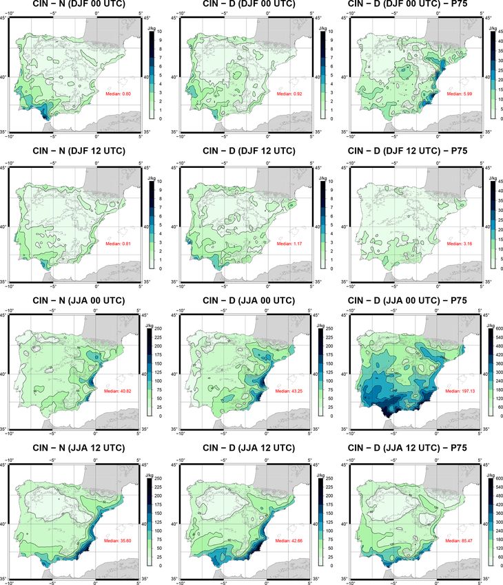
3472                            S. J. González-Rojí et al.: Changes in the simulation of atmospheric instability over the IP

convective precipitation is frequently associated with precip-      Kingdom (Holley et al., 2014) suggests that the reduction of
itation extreme events due to high intensity over a short dura-     CAPE overnight is over 500 J/kg.
tion. However, the simulation of these events is a well-known          On the global scale, CAPE follows the spatial pattern of
problem in the modelling community (Sillmann et al., 2013)          surface specific humidity and air temperature, which means
due to restrictions in the resolution, poor representation of       that it increases from pole to Equator (Riemann-Campe et al.,
complex topography, insufficient assimilated observations,          2009). The minimums are obtained in arid regions and over
forecast errors, or deficiencies in the microphysics schemes        areas with cold water upwelling. Focusing on Europe, con-
in the numerical models. In order to avoid these problems, as       vective storms develop for lower values than the United
previously done in the literature (Viceto et al., 2017), this pa-   States (Graf et al., 2011), and several studies have tried to
per focuses on the evaluation of the atmospheric conditions         determine the most active regions. Amongst them, Romero
favourable for the development of convective precipitation          et al. (2007) found that the region with highest instability is
rather than the validation of the simulation of extreme events.     located along a zonal belt over south-central Europe, partic-
   The evaluation of the atmospheric conditions is typically        ularly over the western Mediterranean Sea and the surround-
based on the calculation of some instability indices such as        ing areas. This agrees with Brooks et al. (2003), who found
the lifted index (LI) (Galway, 1956), the K index (George,          that the favourable environment for thunderstorms is devel-
1960), the total totals index (TT) (Miller, 1972), or the           oped in southern Europe and that the highest number of days
Showalter index (S) (Showalter, 1953). These conditions can         in such a regime is located over the Iberian Peninsula (here-
be also evaluated by convective available potential energy          after, IP), south of the Alps, and the northern Balkans. How-
(CAPE) (Moncrieff, 1981) or convective inhibition (CIN)             ever, van Delden (2001) found that southwestern France and
(Moncrieff, 1981). All of these variables are commonly used         the Basque Country seem to be a preferred region for the for-
in the literature for these kind of studies (e.g. Ye et al.,        mation of severe storms that drift towards the northeast. More
1998; DeRubertis, 2006; Viceto et al., 2017). CAPE and CIN          recent studies based on lightning data (Enno et al., 2020) and
are based on the adiabatic lifting of a parcel, while most          regional climate models using higher resolution (Mohr et al.,
of the others are based on differences in the values of sev-        2015; Rädler et al., 2018) highlighted the same areas with
eral variables at different pressure levels. The deep convec-       favourable environments for thunderstorms in Europe, which
tion is caused by three ingredients: high levels of moisture        are located in particular over northern Italy (Po Valley), east
in the planetary boundary layer (PBL), potential instability,       of the Adriatic Sea (Albania, Bosnia, and Serbia), and in the
and forced lifting (Johns and Doswell, 1992; McNulty, 1995;         northeastern IP and southern France (near the Gulf of Lyon).
Holley et al., 2014; Gascón et al., 2015). CAPE and CIN pro-           Over the IP, the seasonality of precipitation is determined
vide information about the first two ingredients (Holley et al.,    by different sources of moisture due to seasonal variations of
2014), and both can give details about the genesis and inten-       the global atmospheric circulation and contrasting climatic
sity of the atmospheric convection (Riemann-Campe et al.,           regions (influenced by the strong topography). Northern and
2009). However, previous studies (Angus et al., 1988; López         western IP are mainly affected by stratiform precipitation
et al., 2001) suggest that CAPE should not be used alone but        during winter, while eastern and southern IP receive great
should be combined with other indices. The final ingredient,        amounts of precipitation during autumn due to convective
which is the forced lifting, is usually caused by the orogra-       activity (Rodríguez-Puebla et al., 1998; Esteban-Parra et al.,
phy (Doswell et al., 1998; Siedlecki, 2009), the convergence        1998; Romero et al., 1999; Iturrioz et al., 2007). Maximum
of horizontal moisture fluxes (McNulty, 1995), or the breezes       precipitation amounts over central IP are measured in early
in coastal regions (van Delden, 2001). Thus, the high spatial       spring (Tullot, 2000).
and temporal resolution is important for these kind of stud-           Previous studies over the IP (Viceto et al., 2017) sug-
ies focusing on the atmospheric convection, and that is why         gest that CAPE shows a high spatio-temporal variability: the
regional simulations are needed (Siedlecki, 2009).                  values in winter and spring over land are small due to the
   The probability of occurrence of convective precipitation        reduced surface temperature, and the differences between
is not the same through the day, and previous studies sup-          Atlantic and Mediterranean regions are remarkable during
port the maximum convection taking place in the afternoon           summer. According to Siedlecki (2009), the mean values
and evening (Siedlecki, 2009; Virts et al., 2013; Piper and         range from below 50 J/kg in the north to between 100 and
Kunz, 2017; Enno et al., 2020). According to van Delden             200 J/kg at the Mediterranean coast (some events can even
(2001), the preferred time in most of western Europe is be-         reach 1000 J/kg). Similar to Romero et al. (2007), Viceto
tween 18:00 and 24:00 UTC, with the exception of the island         et al. (2017) also stated that CAPE is low during autumn in
of Corsica, where the sea breeze usually causes convection          the Atlantic and continental regions but high in the areas sur-
between 06:00–12:00 UTC. In open-sea areas, the lightning           rounding the Mediterranean Sea. This seasonality was also
activity peaks in the morning (Enno et al., 2020), associated       observed for other indices such as the K index or TT, which
with thunderstorms caused by land breezes at night (Virts           show maximum values during summer (Siedlecki, 2009).
et al., 2013). A regional study that focused over the United        Observations proved that annual precipitation over eastern
                                                                    stations is mostly accumulated during autumn, as a result

Hydrol. Earth Syst. Sci., 25, 3471–3492, 2021                                        https://doi.org/10.5194/hess-25-3471-2021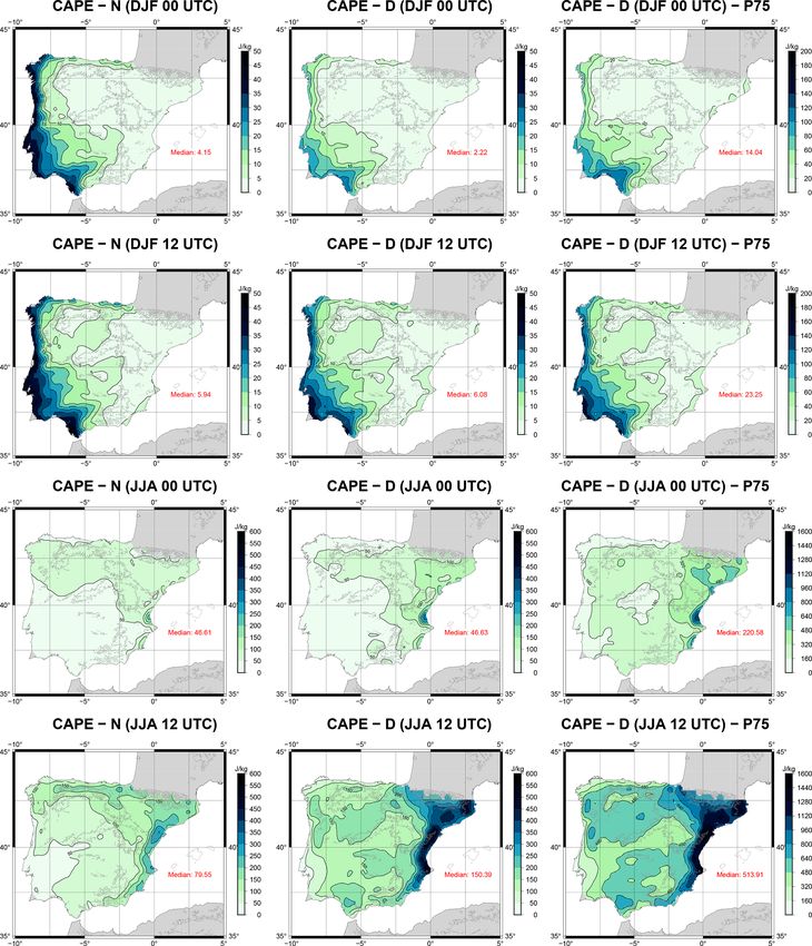
S. J. González-Rojí et al.: Changes in the simulation of atmospheric instability over the IP                                  3473

of the cumulative warming of the Mediterranean Sea due to           iar with the data assimilation process, its main objective is to
summer insolation (Romero et al., 2007; Iturrioz et al., 2007)      produce more reliable and accurate initial conditions for re-
and later entry of very hot and humid air into the IP, while        gional models. This is achieved once the effect of the assimi-
cold air is present at higher levels (Dai, 1999; Eshel and Far-     lated observations is used to modify the fields of temperature,
rell, 2001; Correoso et al., 2006). Additionally, September         wind, and pressure in order to make them closer to the obser-
and October are the months with the highest frequency of            vations. The impact of the data assimilation is not restricted
waterspouts and tornadoes near the Balearic Islands (Gayà           only to the location of the observations being assimilated.
et al., 2001). Over the northwestern IP, the mean value of          First, the improvements due to the analysis are propagated
CAPE when hailstorms occur is 360 J/kg, while for thun-             zonally, meridionally, and vertically to the nearby grid points
derstorms it is only 259 J/kg (López et al., 2001). The dis-        of the domain by means of the background error covariance
persion of these values is really high (almost 350 J/kg over        matrix (Barker et al., 2004, 2012). Second, after the simula-
the whole sample), which is similar to that found in previ-         tion in the new cycle is performed from the initial conditions
ous studies (Alexander and Young, 1992; Lucas et al., 1994).        achieved through assimilation, they propagate in the next 6 h
The values are similar to those observed in other regions of        by means of advection, thus affecting areas distant from the
Europe but lower than those values obtained in studies based        original observations.
on synoptic or lightning data for severe hailstorms (around            This paper is organized as follows: the details of the con-
500 J/kg) (Kunz, 2007; Púčik et al., 2015; Taszarek et al.,        figuration of the WRF model used in both experiments are
2017). Due to global warming, the conditions necessary for          presented in Sect. 2, along with a brief outline of the method-
the development of extreme precipitation events will be en-         ologies used in the study. The main results are presented in
hanced (Brooks, 2013; Rädler et al., 2019). The frequency           Sect. 3, while they are compared against previous studies pre-
and intensity of climate extremes will be magnified (Diff-          sented in the Introduction. Finally, we conclude with some
enbaugh et al., 2013), projecting larger values of CAPE at          remarks about our research in Sect. 4.
the Mediterranean coast during summer and autumn (Marsh
et al., 2009; Viceto et al., 2017).
   The main objective of this paper is to evaluate the perfor-      2     Data and methodology
mance of two simulations created using the Weather and Re-
search Forecasting (WRF) model (Skamarock et al., 2008)             2.1    WRF model configuration
(including or not including the extra 3DVAR data assimi-
lation step) in reproducing the atmospheric conditions that         Two experiments were carried out using version 3.6.1 of
can cause convective precipitation over the IP if the third in-     the WRF model for the period 2010–2014. In both simula-
gredient (e.g. lifting) is fulfilled. We are not restricting our    tions, ERA-Interim provides the initial and boundary condi-
analysis only to convective situations, and the entire period       tions (Dee et al., 2011). Six-hourly data at 0.75◦ were down-
from 2010–2014 will be considered. For the evaluation, the          loaded from the Meteorological Archival and Retrieval Sys-
comparison of pseudo-soundings extracted from the model             tem (MARS) repository at the European Centre for Medium-
against real observations will be carried out. Additionally,        Range Weather Forecasts (ECMWF). Analyses of temper-
the seasonal patterns of different variables commonly used          ature, relative humidity, both horizontal wind components,
to represent atmospheric instability will be studied. More-         and geopotential height at 20 pressure levels (5, 10, 20, 30,
over, this study will also help us to accurately determine the      50, 70, 100, 150, 200, 250, 300, 400, 500, 600, 700, 800,
regions of the IP more prone to developing unstable ther-           850, 900, 925, 950, 1000 hPa) were used to feed WRF. Both
modynamic conditions. If the condition of the forced lifting        simulations were started on the 1 January 2009 from a cold
is also fulfilled, convective precipitation may occur in those      start. Following similar methodologies to previous studies
areas. As shown before, atmospheric instability is a highly         (Argüeso et al., 2011; Zheng et al., 2017), the entire year
demanding feature in model simulations and a topic with             2009 was selected as the spin-up for the land surface model
great importance nowadays due to the large damage that ex-          included in WRF, and consequently, it was omitted in the
treme convective events can cause to society and of which           study presented here.
frequency will be increased in the future. Thus, it is of great        One of the experiments (hereafter, N) was nested in-
interest to diagnose the ability of particular configurations of    side ERA-Interim as usual in numerical downscaling experi-
a model to properly simulate the structure of temperature and       ments, which means that the model is driven by the boundary
moisture at low levels, which lead to atmospheric instability.      conditions after its initialization. It is generated running 6 h
   The novelty of this study lies in the inclusion of the data      long segments that are restarted from the restart file produced
assimilation step in the downscaling experiment used for the        at the end of previous segment, which is similar to a contin-
analysis of some instability indices, as most of the previous       uous WRF run where the boundary conditions are provided
studies are mainly based on simulations driven by bound-            to the model every 6 h after the initialization of the model.
ary conditions after its initialization (e.g. Marsh et al., 2009;   The other experiment (D) relies on the same setup but with
Holley et al., 2014; Mohr et al., 2015). To those not famil-        the additional 3DVAR data assimilation step (Barker et al.,

https://doi.org/10.5194/hess-25-3471-2021                                        Hydrol. Earth Syst. Sci., 25, 3471–3492, 2021
3474                             S. J. González-Rojí et al.: Changes in the simulation of atmospheric instability over the IP

                                                                      ary layer scheme (Nakanishi and Niino, 2006), the Tiedtke
                                                                      cumulus convection scheme (Tiedtke, 1989; Zhang et al.,
                                                                      2011), the RRTMG scheme for both long- and shortwave
                                                                      radiation (Iacono et al., 2008), and the Noah land surface
                                                                      model (Tewari et al., 2004).
                                                                         The background error covariance matrices were created
                                                                      before running the simulation with 3DVAR data assimilation.
                                                                      To do so, the CV5 method included in WRFDA (Parrish and
                                                                      Derber, 1992) was used. A separate simulation initialized at
                                                                      00:00 and 12:00 UTC and spanning 13 months (from Jan-
                                                                      uary 2007 to February 2008) was necessary for the calcu-
                                                                      lation of these matrices. Independent matrices were created
                                                                      for each month, and each of them was calculated taking into
                                                                      account a 90 d period centred on each month.
                                                                         Both simulations were already presented and validated in
                                                                      previous studies by the authors. Integrated water vapour, pre-
                                                                      cipitation, and evaporation over the IP were validated against
Figure 1. The domain used in both WRF simulations is presented        station measurements and gridded datasets including inde-
with dark orange dots, while the dark blue region highlights the      pendent satellite data in González-Rojí et al. (2018), and the
relaxation zone. The location of all the radiosondes available over
                                                                      outputs produced by D were always superior to N and the
the IP is also presented with quartered circles.
                                                                      driving reanalysis ERA-Interim (for the latter, at least com-
                                                                      parable for some variables). The closure of the water balance
                                                                      was also better for D. Additionally, the precipitation from D
2004, 2012) that is run every 6 h (at 00:00, 06:00, 12:00,            exhibited similar capabilities to the one downscaled with sta-
and 18:00 UTC). In this case, 12 h long segments starting             tistical methods (González-Rojí et al., 2019). Furthermore,
at every analysis time (00:00, 06:00, 12:00, and 18:00 UTC)           the wind field from D also showed improvements compared
are used. The analyses are generated from the outputs of the          to ERA-Interim, and, consequently, those data were used for
model at a 6 h forecast step from the previous segment as             the calculation of the offshore wind energy potential in the
first guess in a 3DVAR data assimilation scheme. In both              western Mediterranean (Ulazia et al., 2017). Afterwards, that
experiments, the outputs are saved every 3 h, which means             study was extended to every coast of the IP (Ulazia et al.,
that analyses (00:00, 06:00, 12:00, and 18:00 UTC) and 3 h            2019). The moisture recycling over the IP was also evalu-
forecasts (at 03:00, 09:00, 15:00, and 21:00 UTC) are in-             ated in González-Rojí et al. (2020a), highlighting the reliable
cluded in our results. In the data assimilation step, quality-        results produced by the experiment including data assimila-
controlled temperature, moisture, pressure, and wind obser-           tion and the importance of moisture recycling at the Mediter-
vations in PREPBUFR format from the NCEP ADP Global                   ranean coast during spring and summer.
Upper Air and Surface Weather Observations dataset (ref-                 The effect of data assimilation on moisture and tempera-
erenced as ds337.0 in NCAR’s Research Data Archive) were              ture was measured by the analysis increments (analysis mi-
included. Only those observations included in a time window           nus background) in González-Rojí et al. (2018). The effect
of 2 h centred in the analysis times were assimilated.                of the data assimilation is more intense at 12:00 UTC com-
   As Fig. 1 shows, the domain focuses over the IP, but it also       pared to the other times and particularly for summer (see
includes parts of Europe, Africa, and the Atlantic Ocean. As          their Fig. 13). The spatial analysis of these values highlights
stated by previous studies (Jones et al., 1995; Rummukainen,          that the effect of data assimilation is not homogeneous over
2010), the setup of the domain used in this study prevents            the IP, and it concentrates mainly in the southeastern IP and
border effects affecting our results as mesoscale systems can         both Guadalquivir and Ebro basins. Southern IP has been al-
develop freely. The spatial resolution of both experiments is         ready highlighted by previous studies as a region where cold
15 km, and they include 51 vertical levels up to 20 hPa in eta        biases are observed in WRF simulations during summer (Fer-
(η) coordinates.                                                      nández et al., 2007; Argüeso et al., 2011; Jerez et al., 2012).
   Apart from the ERA-Interim data, sea surface temperature           The fact that the effect of data assimilation is concentrated in
(SST) of the model was updated on a daily basis using the             that region in our WRF simulations is not a coincidence, and
high-resolution dataset NOAA OI SST v2 (Reynolds et al.,              thus, the data assimilation helps to reduce that bias to some
2007) developed by the National Oceanic and Atmospheric               extent.
Administration (NOAA). Additionally, the following param-
eterizations for the physics of the model were included in
both WRF simulations: the five-class microphysics scheme
(WSM5) (Hong et al., 2004), the MYNN2 planetary bound-

Hydrol. Earth Syst. Sci., 25, 3471–3492, 2021                                          https://doi.org/10.5194/hess-25-3471-2021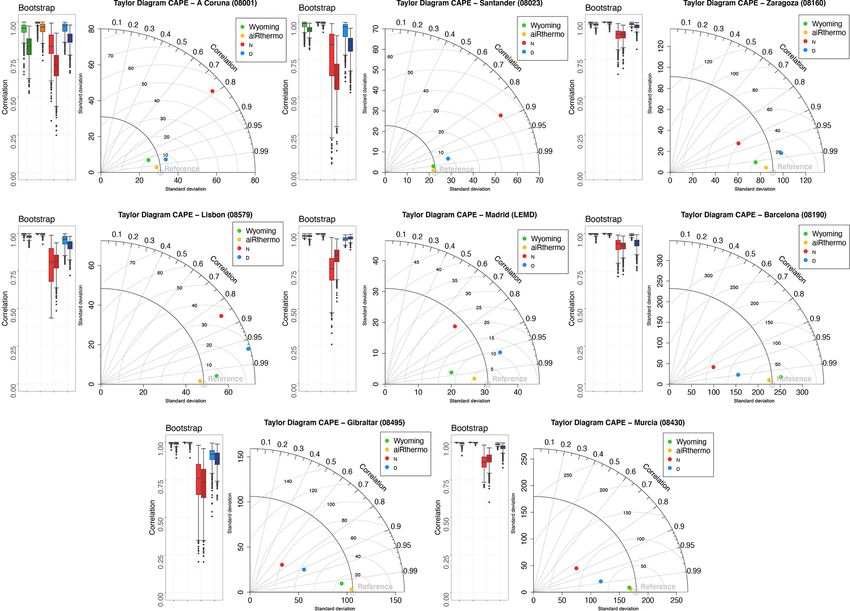
S. J. González-Rojí et al.: Changes in the simulation of atmospheric instability over the IP                                 3475

2.2   Radiosonde data                                                Moreover, we also assume that these radiosondes were
                                                                  very likely assimilated in ERA-Interim. Nevertheless, the im-
Atmospheric radiosonde data were downloaded from the              pact of this is insignificant in our simulations as we only used
server of the University of Wyoming (freely accessible at         ERA-Interim data as boundary conditions for our regional
http://weather.uwyo.edu/upperair/sounding.html, last access:      model after the initial run (1 January 2009). We only anal-
25 September 2019). Even if the University of Wyoming             ysed the outputs from the model after 1 year of spin-up, so
does not apply any quality control to the data, this dataset      the results are only taking into account the variability corre-
was already used in previous studies by the authors, and none     sponding to the regional climate model.
of the values were taken as erroneous. Moreover, data from
the Integrated Global Radiosonde Archive (IGRA) created           2.3     Methodology
by NOAA were also included in this study. This dataset is
constructed by applying different quality control procedures      2.3.1    Calculation of parameters representing
to the raw data. The refined version is then available online.             atmospheric instability
   Only eight radiosondes are available over the IP: A Coruna
(ACOR), Santander (SANT), Zaragoza (ZAR), Barcelona               For both simulations, the nearest grid point to the real lati-
(BCN), Madrid (MAD), Lisbon (LIS), Gibraltar (GIB), and           tude and longitude of each radiosonde was determined, and
Murcia (MUR). The location of each station is presented in        the corresponding pseudo-sounding (pressure, temperature
Fig. 1. Measurements are carried out every day at midday and      and mixing ratio) at 00:00 and 12:00:00 UTC was obtained
midnight (00:00 and 12:00 UTC, corresponding to 02:00 and         at WRF’s original η levels. We did not consider the aver-
14:00 LT summer time, respectively), with the exception of        aged value of several grid points as we would be considering
Lisbon where they are only available at 12:00 UTC (13:00 LT       an extremely large area to be compared against radiosonde
summer time). Additionally, the amount of data available for      data. For example, if we consider an array of 3 × 3 grid
Gibraltar has been extremely scarce since August 2012.            points, we would be taking into account an area of 2025 km2
   Temperature and mixing ratio were retrieved at all the         (45 km × 45 km, as the horizontal resolution of our domain is
available pressure levels at each location from the Univer-       15 km), which is not suitable to be compared against in situ
sity of Wyoming database and from the IGRA dataset. More-         data. Additionally, according to Xu et al. (2015), for every
over, the values of TT, CAPE, and CIN as calculated directly      sounding balloon, the vertical profile of the atmosphere up
by the creators were also retrieved. However, only the val-       to 6 km is already measured for a drifting distance of 7.5 km
ues computed from the IGRA dataset were assumed as the            (half the spatial resolution we use), even if the samples are
reference in our analysis. Additionally, vertical profiles of     taken during a clear or cloudy day (see their Fig. 6). That
temperature and mixing ratio downloaded from the Univer-          means that our spatial resolution is suitable for the direct
sity of Wyoming were also used to calculate TT, CAPE, and         comparison of the nearest points against radiosonde data,
CIN following our own methodology using the aiRthermo R           as we do not neglect the horizontal drift of the sounding
package (further details can be found in the next subsection).    balloons. Thus, averaging the neighbour grid points would
The comparison between the original values of the indices re-     be suitable for the validation of results when convection-
trieved and our results can give us information about whether     permitting scales are used but not in our case as the spatial
their discrepancies are only due to differences in the calcula-   resolution of our model run is 15 km.
tion procedure.                                                      Extracting pseudo-sounding from reanalysis or model data
   It must be said that all the radiosondes presented here        is nothing new, and Lee (2002) or Molina et al. (2020)
were assimilated during the 3DVAR data assimilation step          amongst others showed that these pseudo-soundings are able
in WRF. However, we do not assimilate directly any of the         to reproduce reasonably well the atmospheric conditions
evaluated parameters or precipitation, as we mainly assimi-       measured by real soundings. However, as highlighted by
late pressure, temperature, humidity, and wind. Additionally,     Holley et al. (2014), this procedure takes into account a sta-
as already stated, only eight radiosondes are available over      tionary column at a fixed time, which can influence the com-
the IP. The validation of the results against the assimilated     parison to real radiosonde data as these measurements are
radiosondes (even if we do not assimilate directly the stud-      not instantaneous and not in a straight vertical line as the bal-
ied variables) can be seen as biased, but we cannot exclude       loons used deviate because of wind.
some of these measurements from the data assimilation pro-           In order to calculate TT, CAPE, and CIN using the pseudo-
cess only to be able to validate the simulation afterwards with   soundings from the model, the R package aiRthermo was
such a reduced amount of data available (e.g. assimilate only     employed (Sáenz et al., 2019). The most recent version
four radiosondes and validate the simulation with the remain-     was selected (version 1.2.1), which is publicly available
ing four radiosondes). Thus, in order to get the most accurate    in the CRAN repository (https://cran.r-project.org/package=
results as possible from the model, all the available measure-    aiRthermo, last access: 20 September 2019). Both CAPE and
ments are used.                                                   CIN are calculated by means of the vertical integrals using
                                                                  discrete slabs defined by the resolution of pressure in the

https://doi.org/10.5194/hess-25-3471-2021                                      Hydrol. Earth Syst. Sci., 25, 3471–3492, 2021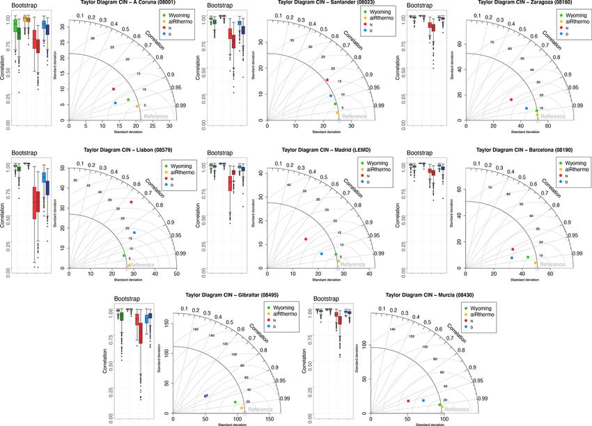
3476                            S. J. González-Rojí et al.: Changes in the simulation of atmospheric instability over the IP

soundings (using all the available levels). The integrals for       mospheric conditions that can cause convection, we needed
each of the slabs enclosed by linear profiles are computed          to restrict our study to a small set of the indices calculated
analytically, and the energy corresponding to each slab is ac-      and provided directly by the radiosonde data holders used in
cumulated, producing the final value of CAPE or CIN. The            this study: IGRA and University of Wyoming. By doing that,
virtual temperature was used in every integral (Doswell and         we can compare our results to those obtained by them and
Rasmussen, 1994). Further details about the functions used          infer which simulation performs better (that including data
for the calculation of the vertical evolution of the air parcels    assimilation or the one without). In both cases, CAPE, CIN,
can be found in Sáenz et al. (2019) and also in the manual of       the TT index, the LI, the S index, or the K index are pro-
the R package aiRthermo associated with that publication.           vided. In the case of the University of Wyoming, SWEAT is
   Additionally, in order to calculate CAPE and CIN in the          also included but not in IGRA. Then, only six indices were
most similar way to the University of Wyoming with the aim          available for us for the validation of our data. The R package
of reducing the differences between the values due to dif-          aiRthermo also allows for the calculation of these six indices,
ferent calculation procedures, the average of the lower verti-      so it was not a restricting feature in our analysis. However,
cal levels was set as the initial representative parcel (Craven     previous studies reported a strong correlation between CAPE
et al., 2002; Siedlecki, 2009; Letkewicz and Parker, 2010).         and LI (Blanchard, 1998; López et al., 2001), and the K index
As in Siedlecki (2009), the averaged values from the low-           is also based on temperature at different pressure levels, so it
est 500 m were used in this study. Furthermore, in order to         suffers from the same problems as TT. Consequently, in or-
avoid the averaged initial parcel state still being too hot com-    der to avoid these connections between indices, we restricted
pared to the ambient conditions (in that case, CIN will never       this study to TT, CAPE, and CIN.
be computed as the parcel is already artificially buoyant), an
isobaric pre-cooling was applied if needed. To do that, the         2.3.2   Analysis
parcel is cooled along an isobar until it crosses the sounding
so that it is not buoyant at the initial state.                     Once TT, CAPE, and CIN are calculated at the nearest grid
   The TT index was calculated following the definition from        points to radiosonde locations of both simulations (N and
Miller (1972). It is defined as                                     D), and also those using the original sounding data from
                                                                    the University of Wyoming (labelled “aiRthermo” in the re-
TT = (T850 − T500 ) + (D850 − T500 ) ,                       (1)
                                                                    sults), we obtain a time series with a 12-hourly temporal
where T850 and T500 are the temperatures at 850 and 500 hPa,        resolution for each index. These values can be compared
and D850 is the dew point temperature at 850 hPa. Accord-           against the reference values of the indices retrieved directly
ing to the ECMWF (Owens and Hewson, 2018), thunder-                 from the University of Wyoming and those computed from
storms are likely when the values for this index are above          the IGRA dataset (labelled “Wyoming” and “Reference”
44◦ C. However, other values can be found in the literature:        respectively in the next figures). The comparison between
48.1◦ C for southern Germany (Kunz, 2007), 46.7 ◦ C for the         Wyoming and aiRthermo aims to achieve an estimation of
Netherlands (Haklander and Van Delden, 2003), or 46 ◦ C for         the error/differences due to the different methods applied by
Switzerland (Huntrieser et al., 1997).                              both sources of results. This comparison was based on in-
   It can be seen that this index is not highly dependent on        dependent locations over the IP (separated by several kilo-
the initial conditions for its calculation as it only depends on    metres), so a Taylor diagram was chosen as the best option
temperature at two discrete pressure levels, while CAPE and         to show the Pearson correlation (r), root mean squared er-
CIN are very sensitive to the initial conditions used for the       ror (RMSE), and standard deviation (SD) of each experiment
simulated ascent. TT avoids this problem, but the results can       in the same plot. In order to determine which experiment is
suffer from errors due to inversion layers (Siedlecki, 2009). It    doing the best job at simulating the reference values of the
must be pointed out that the dew point temperature is needed        variables, the procedure explained by Taylor (2001) was fol-
for TT and that it is highly important for the calculation of the   lowed: the dots that lie nearest to the reference on the x axis
lifting condensation level (LCL) while calculating CAPE and         represent variables that agree well with observations (high
CIN. In the case of the radiosonde data, the indices are cal-       correlations and low RMSEs), and those lying near the high-
culated using the measured dew point temperature at 850 hPa         lighted arc will present comparable standard deviations to the
when is needed, while in our method, this variable is calcu-        observations.
lated from the temperature and mixing ratio at that pressure           Additionally, the bootstrap technique with resampling was
level. This can cause small differences in the results, even if     applied to the results in order to represent an estimation of
the same original radiosonde data are used.                         the sampling errors from each experiment (Efron and Gong,
   Further indices could be calculated from the pseudo-             1983; Wilks, 2011). In our case, the original time series used
soundings obtained from the outputs of the model or real            in the Taylor diagrams consist of 60 values, each of them
observations. However, keeping in mind that the main ob-            for the corresponding month along the period 2010–2014
jective of this study is to evaluate the difference in the per-     (12 months × 5 years). For the bootstrap, we created 1000
formance of two simulations in reproducing the unstable at-         perturbed time series taking into account different samples

Hydrol. Earth Syst. Sci., 25, 3471–3492, 2021                                        https://doi.org/10.5194/hess-25-3471-2021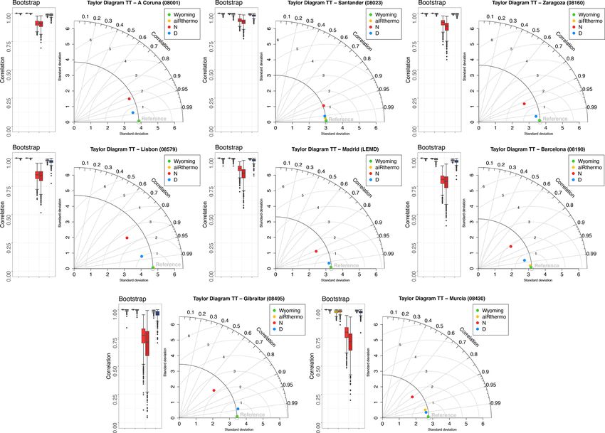
S. J. González-Rojí et al.: Changes in the simulation of atmospheric instability over the IP                                  3477

of the data. A total of 67 % of the new time series (2/3 of the      underestimates it at most of the stations as it is only able to
length of the original time series – 40 values in our case) is       reproduce the one in Santander and A Coruna. The RMSE
made from the original data, and the remaining 33 % (1/3–            is below 0.6 ◦ C for aiRthermo, below 1 ◦ C for D, and below
20 values) is chosen from those values already taken from the        2.5 ◦ C for N.
original data. For each correlation calculated, the same sam-           The bootstrap analysis is consistent with the results ob-
ples are taken from all datasets and experiments. The vari-          tained in the Taylor diagrams, and it shows that the Pearson
ability of the Pearson and Spearman correlations obtained            correlations are always above 0.99 for Wyoming and 0.98 for
with these synthetic time series was shown by means of box-          aiRthermo (again, with the exception of Murcia, where they
and-whisker plots.                                                   are above 0.9). The correlations are always above 0.95 for
   Then, the seasonal analysis of each parameter at each loca-       D. In the case of N, the spread of the values is much larger
tion was carried out. In this case, the variability of the results   than for aiRthermo and D, and their median values are ob-
is showed by different box-and-whisker plots. Each season            tained between 0.8 and 0.9. If we change to Spearman’s cor-
was defined as follows: winter is defined from December to           relations, we can see that values are similar but with a small
February (DJF), spring from March to May (MAM), sum-                 decrease of the values (particularly in Gibraltar, Murcia, and
mer from June to August (JJA), and autumn from September             Madrid).
to November (SON).                                                      Thus, as expected, we obtain the most similar results to
   The main objective of this paper was to analyse the abil-         those calculated from IGRA (Reference) with the values
ity of the model to properly simulate atmospheric conditions         from Wyoming and those calculated with the real measure-
by means of TT, CAPE, and CIN. Thus, the calculation of              ments from the soundings (that is, aiRthermo). However, we
TT, CAPE, and CIN was extended to every grid point in-               can still detect small differences between the values of the
cluded in a mask defined for the land points of the IP over          datasets due to the use of measured dew point temperature in
the model’s domain. The spatial distribution of the mean val-        Wyoming, whilst it is computed from temperature and mix-
ues of them at 00:00 and 12:00 UTC during winter and sum-            ing ratio in IGRA and aiRthermo. These differences are more
mer was calculated. These maps show the spatial distribution         remarkable in Murcia. Between both WRF experiments, it
of TT, CAPE, and CIN over the land grid points in the IP             is clear that the experiment including the 3DVAR data as-
which are more prevalent in each season. However, from the           similation is able to outperform the standard simulation only
point of view of the applicability of these results to the evalu-    driven by the reanalysis data at the boundaries of the do-
ation of unstable atmospheric conditions, it is also important       main (N). The differences between both WRF simulations
to analyse the joint distribution of CAPE and CIN limited to         are highlighted, particularly at those stations located at the
those days characterized by high values of CAPE. In order to         Mediterranean coast (Barcelona, Murcia, and Gibraltar) and
select those days, the 75th percentile of CAPE at every grid         in Lisbon.
point, season of the year, and time (00:00 and 12:00 UTC)               In the case of CAPE, the validation results are presented
was used as a threshold. Only those days on which CAPE               in Fig. 3. The best experiment reproducing the results is
was above this percentile (labelled P75) were considered to          aiRthermo, followed by Wyoming, D, and finally by N. The
calculate the mean value of CAPE and CIN.                            correlations are at all the stations above 0.99 in aiRthermo
                                                                     and 0.95 for Wyoming, while for D they are above 0.9 and
                                                                     above 0.7 for N. A similar behaviour is observed for SD and
3   Results                                                          RMSE. The largest RMSEs are obtained for Barcelona and
                                                                     Murcia (both in the Mediterranean region).
Taylor diagrams for the TT index calculated for each ra-                The bootstrap analysis shows that the highest Pearson cor-
diosonde of the IP are shown in Fig. 2. The box-and-whisker          relations are obtained by aiRthermo and Wyoming but fol-
plots associated with the correlations (both the Pearson and         lowed really closely by D. As for the TT index, N presents
Spearman) obtained for each of the 1000 time series created          the worst performance and the largest spread. If we consider,
with the bootstrap technique are also included. According            instead, the use of Spearman’s correlations, we can see that
to the Taylor diagrams, the best experiment reproducing the          the values are similar at most of the stations, and only in
reference values is Wyoming, followed by aiRthermo (the              A Coruna and Santander is there a strong decrease of the
real measurements of temperature, mixing ratio, and pres-            values.
sure from the sounding were used to calculate TT with our               As stated before in Sect. 2.3.1, the calculation of CAPE
methodology), D, and later by N. Wyoming obtains the clos-           is more sensitive to subtle differences in the methodology
est values to the observations at all the stations. The results      than that of TT, and this is highlighted in the validation of
for aiRthermo are quite similar to Wyoming, except for Mur-          these results. Even if the same data are used for the calcu-
cia, where D is better at reproducing the reference data. The        lation of CAPE (Wyoming and aiRthermo used the same
correlations are always above 0.99 for Wyoming, 0.98 for             measurements as input), it is clear that small differences
aiRthermo, 0.97 for D, and 0.75 for N. The observed SD is            in the initial conditions can result in serious discrepancies
really well simulated by Wyoming, aiRthermo, and D, but N            between both methods as stated by Siedlecki (2009). The

https://doi.org/10.5194/hess-25-3471-2021                                         Hydrol. Earth Syst. Sci., 25, 3471–3492, 2021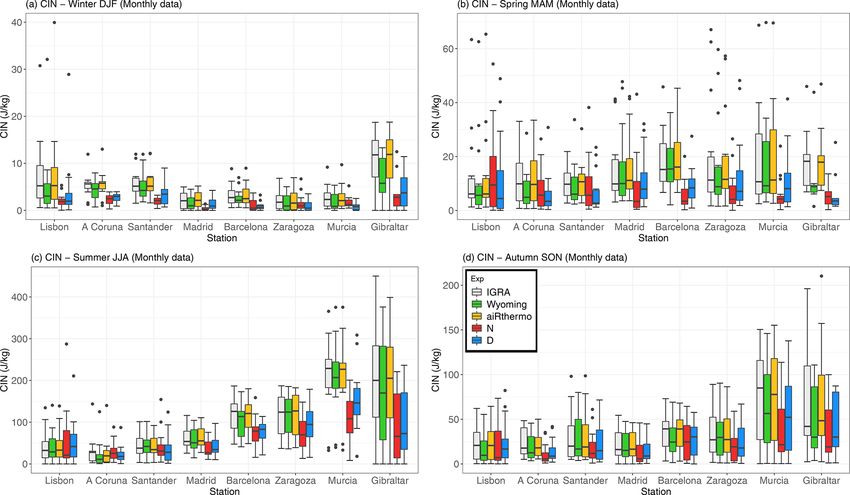
3478                             S. J. González-Rojí et al.: Changes in the simulation of atmospheric instability over the IP

Figure 2. Taylor diagrams showing the r, RMSE, and SD values for Wyoming, aiRthermo, N, and D compared to TT values computed from
IGRA (Reference). On the left side of each Taylor diagram, a box-and-whisker plot is added in order to show the Pearson and Spearman
correlations between each experiment and the reference data (lighter and darker colours, or first and second columns of the box-and-whisker
plots respectively). The bootstrap technique with resampling was used to create 1000 synthetic time series. Wyoming, aiRthermo, N, and D
are plotted in green, orange, red, and blue respectively.

largest RMSEs for aiRthermo can be found at Barcelona and               tively. Both WRF experiments overestimate or underestimate
Murcia. As for the TT index, two stations at the Mediter-               it depending on the station (particularly N in Lisbon, Madrid,
ranean coast present the largest differences between the ex-            Murcia, and Zaragoza). The RMSE is always larger for N and
periments. However, while the computation of TT from both               particularly in Murcia and Gibraltar, where the values exceed
WRF simulations produces standard deviations similar to the             40 J/kg.
observed ones, the results for CAPE substantially overesti-                The bootstrap analysis presents the same results as for
mate the variance of Atlantic sites (A Coruna, Santander,               CAPE (Fig. 3). However, for Gibraltar, as shown in the Tay-
and Lisbon) and Madrid or underestimate it at the Mediter-              lor diagram, both WRF experiments produce a similar Pear-
ranean coast (Barcelona, Murcia, and Gibraltar). In any case,           son correlation values during the bootstrap. If we consider,
it can be seen that data assimilation improves the simulation           instead, Spearman’s correlations, the worse performance of
of CAPE over the IP.                                                    N is perceptible in A Coruna, Santander, Murcia, and Gibral-
   Finally, the validation of CIN is presented in Fig. 4. As for        tar. However, in Gibraltar, differences between both WRF
CAPE, the best results are obtained again by aiRthermo, fol-            experiments arise: WRF D obtained better correlations than
lowed by Wyoming, D, and N (with the exception in Gibral-               WRF N as in the other stations. In contrast to previous re-
tar, where D and N are really similar). aiRthermo obtains cor-          sults, the poorest correlations for CIN are obtained at stations
relations above 0.97 in every station, followed by Wyoming,             located at the Atlantic coast as Lisbon and A Coruna.
D, and N with correlations above 0.93, 0.85, and 0.65 respec-

Hydrol. Earth Syst. Sci., 25, 3471–3492, 2021                                             https://doi.org/10.5194/hess-25-3471-2021
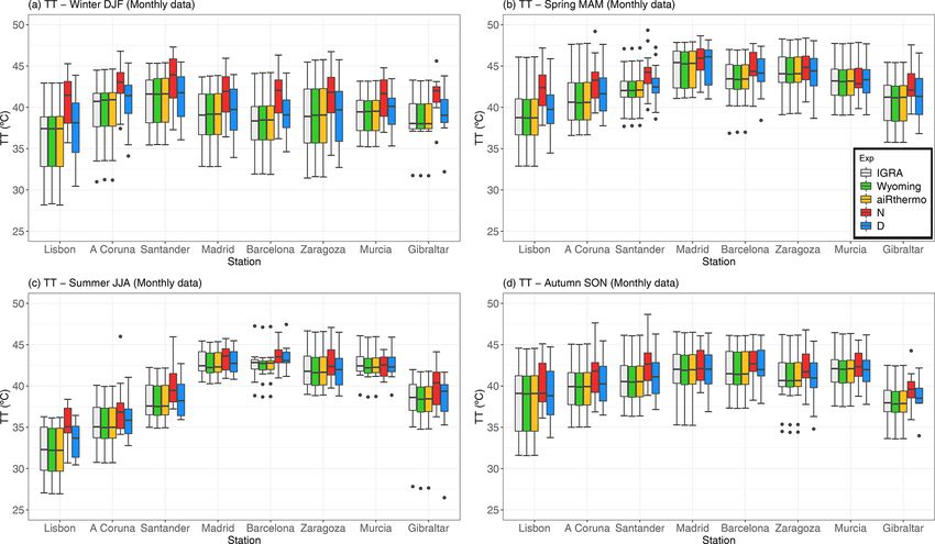
S. J. González-Rojí et al.: Changes in the simulation of atmospheric instability over the IP                                 3479

Figure 3. Same as Fig. 2 but for CAPE.

   As for CAPE, the differences between aiRthermo and                ture at 500 hPa. As shown by Fig. S1, the winter temperature
Wyoming are highlighted here. This result supports the idea          at 850 hPa is higher for D than for N, but this would lead to
that small differences in the initial conditions of the lifted air   higher values of TT, so that it does not explain the observed
parcel and the determination of the LCL due to differences in        discrepancies for the N simulation. For the case of dew point
the dew point temperature can cause large differences in the         temperature at 850 hPa (Fig. S2), it is higher for the N simu-
values of CIN, even if the same vertical profile of tempera-         lation than for D, which leads to higher values of TT for N.
ture and mixing ratio are used for its calculation. Again, the       Additionally, the temperature at 500 hPa is higher for D than
differences between both WRF experiments are important,              for N, and this also leads to higher values of TT for N than
and the experiment including data assimilation (D) presents          for D. It is, thus, clear that the improvement in the simula-
generally closer results to the observed ones.                       tion of TT during winter for the D simulation is due to an
   The seasonal analysis of the five datasets (Reference,            improved simulation of moisture and temperature at the low
Wyoming, aiRthermo, N, and D) for the TT index is pre-               (850 hPa) and middle troposphere (500 hPa) derived from the
sented in Fig. 5. In this case, Wyoming, aiRthermo, and D            assimilation of soundings. The same diagnostic can be done
are able to correctly simulate the reference seasonal variabil-      for spring, another season during which N overestimates TT
ity of the TT index at all the stations and all the seasons.         in many of the soundings (A Coruna, Santander, Lisbon, and
However, N tends to overestimate the values of TT in every           Barcelona). They are located in areas where the difference
season and for most of the stations over the IP. The difference      between the dew point temperature from simulation D minus
in TT is most important during winter months as a severe             the one from N is negative (see Fig. S2).
overestimation by the simulation N without data assimilation            A Coruna and Santander present the largest values dur-
can be seen. It can be tracked on the basis of Figs. S1–S3 (in       ing winter. Higher values than in winter are observed during
the Supplement) to an improved representation of tempera-            spring, and the maximum is recognizable in Madrid, which is

https://doi.org/10.5194/hess-25-3471-2021                                         Hydrol. Earth Syst. Sci., 25, 3471–3492, 2021
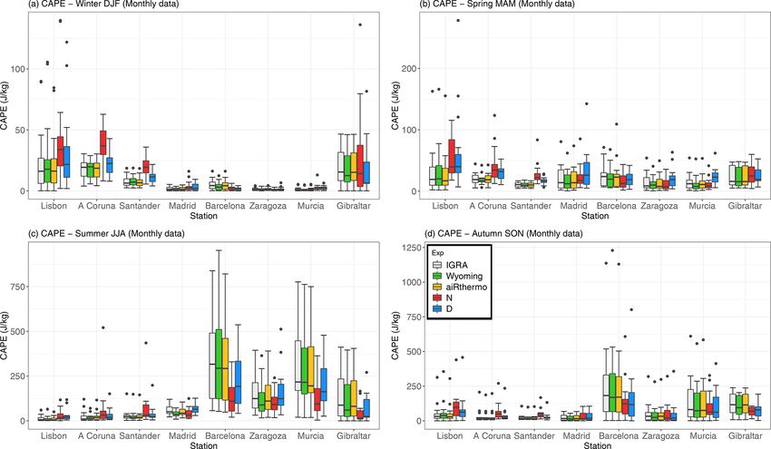
3480                             S. J. González-Rojí et al.: Changes in the simulation of atmospheric instability over the IP

Figure 4. Same as Figs. 2 and 3 but for CIN.

the only station located over central IP. Even if the maximum       at most of the stations during winter, summer, and autumn.
is found there, the other stations also present values above        However, both WRF experiments (particularly D) overesti-
38 ◦ C. During summer, central, eastern, and southern stations      mate CAPE at most of the stations in spring due to the differ-
(Madrid, Barcelona, Zaragoza, and Murcia) are the ones pre-         ences in the virtual temperature in lower levels compared to
senting higher values. In that season, the Atlantic stations        reference data (colder near surface and warmer near 800 hPa)
(A Coruna and Santander) and Gibraltar present values be-           and with lifted parcels for D slightly warmer than the refer-
low 40 ◦ C. The values of TT in summer at those stations are        ence ones and those for N (see Fig. S4).
smaller than the ones in winter, which occurs mainly due to            The experiment without data assimilation (N) tends to
the combined effect of the high increasing values of temper-        overestimate CAPE in winter and to underestimate it in sum-
ature at 850 and 500 hPa (about 15 and 10◦ respectively) and        mer. In winter, this overestimation is caused mainly by colder
the smaller increase of dew point temperature (only a few de-       conditions in the 850–750 hPa pressure levels and warmer
grees) in those regions from winter to summer (see Figs. S1–        lifted air parcels (particularly in Lisbon, A Coruna, and San-
S3 in the Supplement). Finally, all the stations show similar       tander – see Fig. S5). A detailed analysis of the vertical struc-
values in autumn, with the exception of Gibraltar where the         ture of the differences of both simulations against IGRA for
values are smaller.                                                 virtual temperature and mixing ratio (Fig. S6) shows that the
   The seasonal analysis for CAPE is presented in Fig. 6, and       vertical structure of moisture is improved in the D simula-
it highlights the spatial and temporal heterogeneity of the ar-     tion, thus leading to a better estimation of CAPE through the
eas where unstable air masses can be observed over the IP, as       troposphere due to improved estimations of virtual tempera-
also shown by Holley et al. (2014). Wyoming and aiRthermo           ture.
are able to reproduce (as expected) the variability of the refer-      On the contrary, in summer, the underestimations of CAPE
ence values, and D is able to capture the spread of the values      by the N simulation are caused by warmer conditions in

Hydrol. Earth Syst. Sci., 25, 3471–3492, 2021                                        https://doi.org/10.5194/hess-25-3471-2021
S. J. González-Rojí et al.: Changes in the simulation of atmospheric instability over the IP                                        3481

Figure 5. TT index for the reference data (grey), Wyoming (green), aiRthermo (orange), N (red), and D (blue), computed at each station for
every season: winter (a), spring (b), summer (c), and autumn (d).

the lower pressure levels compared to the reference, which             ern and southern parts of the IP present remarkable values
causes the lifted parcel to cross the sounding in a lower pres-        of CAPE. Particularly, the highest CAPE values are located
sure level than D, consequently underestimating CAPE (par-             at the Mediterranean coast (Barcelona and Murcia). Finally,
ticularly for Barcelona, Murcia, and Gibraltar – see Fig. S7).         during autumn, the regions with high CAPE are extended to-
A detailed analysis for Barcelona (Fig. S8) shows that there           wards the inland of the IP, such as Madrid and Zaragoza.
is a substantial underestimation of moisture at lowest levels          During this season, some extreme events can reach values
by the N simulation, something which is consistent with find-          over 1000 J/kg over the Mediterranean coast. This feature
ings in González-Rojí et al. (2018) in a verification with in-         was already observed by Siedlecki (2009). All these seasonal
dependent non-assimilated MODIS-integrated water vapour.               changes in CAPE also agree with previous studies based on
This is also observed in Murcia (figure not shown). During             CAPE (Romero et al., 2007; Viceto et al., 2017).
spring and autumn, the underestimations or overestimations                Finally, the seasonal analysis for CIN is presented in
of N depend on the station, and a clear pattern is not ob-             Fig. 7, and it highlights the stations where the inhibition is
served.                                                                important. In general, Wyoming tends to underestimate the
   The lowest values of CAPE are obtained during winter                values of CIN at most of the stations and in every season,
(below 50 J/kg at all the stations), and the largest ones are ob-      while aiRthermo is able to capture it. Both WRF simulations
served in summer (reaching 500 J/kg at some stations). How-            (but particularly the experiment without data assimilation)
ever, as stated before, the distribution of CAPE is not ho-            tend to underestimate the observed variability.
mogeneous, and different regions are prone to higher values               The values of CIN are smaller in winter and spring, and
during each season. During winter, the three Atlantic stations         the maximum is observed in summer. During winter, CIN
(A Coruna, Santander, and Lisbon) and Gibraltar present the            is higher in Gibraltar and at the Atlantic stations (Lisbon,
highest values of CAPE over the IP. In general, the values are         A Coruna, and Santander) than at the other stations from the
below 50 J/kg, but some events can exceed 100 J/kg. During             IP. However, these values are small compared to those for
spring, the distribution of CAPE is quite homogeneous over             other seasons. During spring, the values are higher than in
the IP and only stations such as Lisbon, Madrid, or Gibral-            winter, and similar values are observed at most of the stations
tar present slightly higher values of CAPE than the other              (around 10 J/kg), with the exception of Barcelona where the
stations. In summer, only the stations located in the east-            CIN reaches values of 20 J/kg. In summer, the values are

https://doi.org/10.5194/hess-25-3471-2021                                            Hydrol. Earth Syst. Sci., 25, 3471–3492, 2021
3482                             S. J. González-Rojí et al.: Changes in the simulation of atmospheric instability over the IP

Figure 6. Same as Fig. 5 but for CAPE.

Figure 7. Same as Figs. 5 and 6 but for CIN.

Hydrol. Earth Syst. Sci., 25, 3471–3492, 2021                                     https://doi.org/10.5194/hess-25-3471-2021
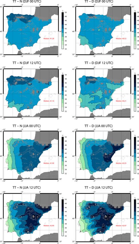
S. J. González-Rojí et al.: Changes in the simulation of atmospheric instability over the IP                               3483

higher at all the stations but particularly in those for the      masses extend towards the central area. In this case, they are
eastern and southern IP (Barcelona, Zaragoza, Murcia, and         located near the Pyrenees and in the proximity of the Iberian,
Gibraltar). The same regime is observed for autumn, but the       Central, and Baetic systems. The minimum TTs are observed
values are smaller than in summer. These values during sum-       in the western part of the IP but particularly near Lisbon. The
mer and autumn are in agreement with Siedlecki (2009), who        intensity of the most extreme values of TT is higher in D
found CIN means above 100 J/kg in the western Mediter-            (with data assimilation).
ranean Sea and surrounding countries.                                The maps of CAPE at 00:00 and 12:00 UTC during winter
   As stated before, in the final phase of this study, the same   and summer are presented in Fig. 9, together with the mean
procedure for the calculation of TT, CAPE, and CIN at each        values of CAPE that are larger than the 75th percentile at
station was extended to each grid point included in the IP.       each point of the domain for the D experiment (P75 col-
The mean winter and summer spatial patterns at 00:00 and          umn). During winter, as shown in Fig. 6, the N experiment
12:00 UTC were calculated for both WRF experiments. In            presents higher values than D. At 00:00 UTC, the patterns are
addition, CAPE and CIN limited to those days character-           really similar for both WRF experiments. The main differ-
ized by high values of CAPE (based on the 75th percentile         ence between them is observed at the western Atlantic coast
of CAPE at each grid point, season of the year, and time –        of the IP, where higher CAPE values are obtained for N. At
00:00 and 12:00 UTC) were also evaluated. These maps were         12:00 UTC, the unstable air masses are found at the western
added to the corresponding figures for CAPE and CIN as a          coast of the IP in both simulations, and they extend further
third column. However, these results are only shown for the       inland than at 00:00 UTC, particularly near the Tagus and
D experiment, the one that was shown to be the most accurate      Guadalquivir rivers. Again, the values are higher for N, but
one according to the Taylor diagrams and seasonal box-and-        the pattern is similar in both experiments. If the analysis is
whisker plots in previous results.                                limited to values of CAPE beyond the third quartile during
   The spatial distribution for TT is shown in Fig. 8, which      winter, the values are higher, but the spatial distribution at
highlights the heterogeneity of the results. The differences      both 00:00 and 12:00 UTC is very similar to the average one
between both simulations are observable but also those be-        from the D experiment.
tween day and night. Additionally, it can be seen that TT            Compared to what is observed during winter, CAPE is
cannot be calculated in most of the mountain regions of the       higher during summer for the experiment including data as-
IP because the 850 hPa layer is near the surface or below         similation. This is in agreement with the station analysis
ground.                                                           shown in Fig. 6. At 00:00 UTC, the area with higher CAPE
   During winter, the maps of TT show that N yields higher        is observed in the northern and eastern IP but particularly
values than D, which is in agreement with the overestimation      near the Mediterranean coast. However, at 12:00 UTC, this
observed in Fig. 5. At 00:00 UTC, according to D, the re-         area with high values (over 250 J/kg) extends towards the
gions where unstable air masses are observed are those at the     interior, and in the experiment including data assimilation
Cantabrian coast and in the southeastern IP. Both regions are     it also covers the southern part of the Pyrenees. Addition-
surrounded by remarkable mountainous systems such as the          ally, high values are observed in most of the IP (except the
Cantabrian Range and the Baetic System, which can trigger         southwestern corner for N) but particularly in the simulation
convection by orographically induced lifting. For N, these ar-    including data assimilation. The patterns of CAPE obtained
eas are also extended to the rest of the IP, with the exception   for both winter and summer are in agreement with those from
of the southwestern corner where the values are small. At         Viceto et al. (2017), even if we differentiate between 00:00
12:00 UTC, after solar irradiance has started heating up the      and 12:00 UTC, and we studied different periods (1986–2005
land, the regions extend towards inland areas. In the experi-     in their study, 2010–2014 in ours). If the focus is set on the
ment with data assimilation (D), most of the northern plateau     days characterized by CAPE higher than the third quartile
presents high values of TT, and the lowest values are ob-         (third column of Fig. 6), it can be seen that, as expected, the
served near the coastal valleys of the southwestern corner        CAPE field is intensified, but the changes in its spatial dis-
and the Mediterranean coast (like the Ebro basin or Murcia).      tribution are not relevant. The Mediterranean region is still
In the case of N, the lowest values are observed mainly in        the one showing the highest values of CAPE, particularly at
the southwestern IP near the Guadalquivir valley. According       12:00 UTC, even though there is a general small increase of
to Figs. S1–S3, the lowest values of TT observed near the         CAPE over the entire IP.
coastal valleys of both WRF experiments are a consequence            Finally, regarding CIN, the maps for the mean values at
of low dew point temperatures there mainly due to dry air.        00:00 and 12:00 UTC during winter and summer are pre-
   As in Fig. 5, much higher TT values are obtained dur-          sented in Fig. 10. In reverse to what we found for CAPE, CIN
ing summer over the IP, particularly at 12:00 UTC. At             is usually higher at 00:00 UTC than at 12:00 UTC (with the
00:00 UTC, a west–east gradient is observed in both WRF           exception of Murcia in summer at 12:00 UTC), as could be
simulations. However, the values depicted at the Mediter-         expected due to the stabilizing effect of nocturnal radiation.
ranean coast are higher for the experiment including data as-     During winter, at 00:00 UTC, both simulations show small
similation (D). At 12:00 UTC, the regions with unstable air       values over the IP, and only some high values are observed

https://doi.org/10.5194/hess-25-3471-2021                                      Hydrol. Earth Syst. Sci., 25, 3471–3492, 2021
You can also read