The 32-year record-high surface melt in 2019/2020 on the northern George VI Ice Shelf, Antarctic Peninsula - The Cryosphere
←
→
Page content transcription
If your browser does not render page correctly, please read the page content below
The Cryosphere, 15, 909–925, 2021
https://doi.org/10.5194/tc-15-909-2021
© Author(s) 2021. This work is distributed under
the Creative Commons Attribution 4.0 License.

The 32-year record-high surface melt in 2019/2020 on the northern
George VI Ice Shelf, Antarctic Peninsula
Alison F. Banwell1,2 , Rajashree Tri Datta3,4,5 , Rebecca L. Dell2 , Mahsa Moussavi6,1 , Ludovic Brucker3,7 ,
Ghislain Picard8 , Christopher A. Shuman3,9 , and Laura A. Stevens10,11
1 Cooperative   Institute for Research in Environmental Sciences (CIRES), University of Colorado Boulder, Boulder, CO, USA
2 Scott  Polar Research Institute (SPRI), University of Cambridge, Cambridge, UK
3 Cryospheric Sciences Laboratory, NASA Goddard Space Flight Center, Greenbelt, MD, USA
4 Earth System Science Interdisciplinary Center, University of Maryland, College Park, MD, USA
5 Department of Atmospheric and Oceanic Sciences (ATOC), University of Colorado Boulder, Boulder, CO, USA
6 National Snow and Ice Data Center (NSIDC), University of Colorado Boulder, CO, USA
7 Goddard Earth Sciences Technology and Research Studies and Investigations, Universities Space Research Association,

Columbia, MD, USA
8 Institut des Géosciences de l’Environnement (IGE), CNRS, Univ. Grenoble Alpes, UMR 5001, 38041 Grenoble, France
9 Joint Center for Earth Systems Technology, University of Maryland, Baltimore County, Greenbelt, MD, USA
10 Department of Earth Sciences, University of Oxford, Oxford, UK
11 Lamont-Doherty Earth Observatory of Columbia University, Palisades, NY, USA

Correspondence: Alison F. Banwell (alison.banwell@colorado.edu)

Received: 18 October 2020 – Discussion started: 22 October 2020
Revised: 12 January 2021 – Accepted: 19 January 2021 – Published: 25 February 2021

Abstract. In the 2019/2020 austral summer, the surface melt      potential for hydrofracture initiation; a risk that may increase
duration and extent on the northern George VI Ice Shelf          due to firn air content depletion in response to near-surface
(GVIIS) was exceptional compared to the 31 previous sum-         melting.
mers of distinctly lower melt. This finding is based on analy-
sis of near-continuous 41-year satellite microwave radiome-
ter and scatterometer data, which are sensitive to meltwa-
ter on the ice shelf surface and in the near-surface snow.       1   Introduction
Using optical satellite imagery from Landsat 8 (2013 to
2020) and Sentinel-2 (2017 to 2020), record volumes of sur-      Since the 1950s, the Antarctic Peninsula (AP) (Fig. 1a) has
face meltwater ponding were also observed on the north-          experienced faster increases in ocean and atmospheric warm-
ern GVIIS in 2019/2020, with 23 % of the surface area            ing than the rest of the Antarctic Ice Sheet (Siegert et al.,
covered by 0.62 km3 of ponded meltwater on 19 January.           2019; Smith et al., 2020; Trusel et al., 2015). The rate of
These exceptional melt and surface ponding conditions in         mass loss from the AP has tripled since the 1990s, with an
2019/2020 were driven by sustained air temperatures ≥ 0 ◦ C      average of 24 Gt yr−1 from 1979 to 2017 and an acceleration
for anomalously long periods (55 to 90 h) from late Novem-       of 16 Gt yr−1 per decade (Rignot et al., 2019). Mass loss is
ber onwards, which limited meltwater refreezing. The sus-        currently focused at marine margins, where the mass balance
tained warm periods were likely driven by warm, low-speed        is controlled by complex interactions between the ice, ocean,
(≤ 7.5 m s−1 ) northwesterly and northeasterly winds and not     atmosphere, and inland bed conditions (Scambos et al., 2000;
by foehn wind conditions, which were only present for 9 h to-    Bell et al., 2018; Shepherd et al., 2018; Tuckett et al., 2019;
tal in the 2019/2020 melt season. Increased surface ponding      Smith et al., 2020). An important part of this system are the
on ice shelves may threaten their stability through increased    ice shelves, which have a total area of ∼ 120 000 km2 around
                                                                 the AP (Siegert et al., 2019) and act to buttress the inland

Published by Copernicus Publications on behalf of the European Geosciences Union.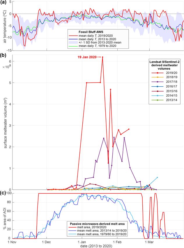
910                        A. F. Banwell et al.: 32-year record-high melt on the northern George VI Ice Shelf, Antarctica

grounded ice flowing into the ocean (Scambos et al., 2004;        2   Study site
De Rydt et al., 2015; Fürst et al., 2016; Gudmundsson et al.,
2019).                                                            GVIIS is located in the southwestern AP between Alexan-
   Ice shelf surface melting, which results in surface lower-     der Island and Palmer Land (Fig. 1). With an area of
ing and (if sustained) thinning (Paolo et al., 2015), is con-     ∼ 23 500 km2 (Rignot et al., 2013), it is the second largest
nected to ice shelf stability as follows. In warm summers,        remaining ice shelf on the AP after the Larsen C. GVIIS has
meltwater produced at the ice shelf surface is stored in the      two ice fronts, separated by ∼ 450 km along its centreline:
perennial snowpack (“firn”). Refreezing of this meltwater         a northern ice front that calves into Marguerite Bay, and a
releases latent heat into the firn, causing additional melt-      southern ice front that terminates into the Ronne Entrance
ing, firn saturation, and firn air content depletion; eventu-     (Holt et al., 2013). GVIIS is structurally complex, with dis-
ally facilitating meltwater ponding on the ice shelf surface      tinct flow units originating in Palmer Land flowing across
(Holland et al., 2011; Kuipers Munneke et al., 2014). Exten-      to, and impinging against, Alexander Island (Reynolds and
sive surface ponding (Kingslake et al., 2017; Arthur et al.,      Hambrey, 1988; Hambrey et al., 2015; Davies et al., 2017),
2020a; Dell et al., 2020) may threaten ice shelf stability due    resulting in a dominantly compressive flow regime (LaBar-
to stress variations associated with overall meltwater move-      bera and MacAyeal, 2011). The ice shelf decelerates as it
ment, ponding, and drainage (Scambos et al., 2000, 2003;          flows westwards across the sound, with ice velocities on the
MacAyeal et al., 2003; Banwell and MacAyeal, 2015; Ban-           northern GVIIS varying from ∼ 400 m yr−1 near the ground-
well, 2017; Banwell et al., 2019). These processes may initi-     ing line to ∼ 30 m yr−1 near Alexander Island (Bishop and
ate meltwater-induced vertical fracturing (“hydrofracturing”)     Walton 1981). This complex flow regime controls ice shelf
(Van der Veen, 2007; Dunmire et al., 2020; Lai et al., 2020),     thickness, which varies from ∼ 100 m at both ice fronts to
especially if the ice shelf is already damaged with a high den-   ∼ 600 m in the centre (Smith et al., 2007; Davies et al., 2017).
sity of crevasses (Lhermitte et al., 2020). The near-complete        Compared to the southern GVIIS (∼ 72◦ 000
collapse of the Larsen B Ice Shelf in 2002 is arguably the        to ∼ 77◦ 000 S), the northern GVIIS (∼ 70◦ 300 to
most famous break-up event due to its rapidity and extent         ∼ 72◦ 000 S) experiences higher surface summer melt
(e.g. Scambos et al., 2003) and may have been driven by the       rates (< 250 mm w.e. yr−1 ; Trusel et al., 2013; Datta et al.,
drainage of ∼ 3000 lakes (Banwell et al., 2013; Robel and         2018) and lower accumulation rates (< 200 kg m−2 yr−1 ;
Banwell, 2019; Leeson et al., 2020). However, surface melt-       Bishop and Walton, 1981; Reynolds, 1981); the latter is at-
ing has also been implicated in the large-scale collapse events   tributed to the presence of a precipitation shadow downwind
of the Prince Gustav and Larsen A ice shelves over just a         of Alexander Island (Bishop and Walton, 1981). As a result,
few days in late January 1995 (Rott et al., 1996; Doake et al.,   winter snowfall on the northern GVIIS rarely lasts through
1998; Scambos et al., 2003; Glasser et al., 2011) and in other,   the summer (Holt et al., 2013), and extensive areas of
smaller-scale collapses of the Wilkins, Larsen B, George VI,      ponded surface water have been observed here since at least
and Larsen A ice shelves (Scambos et al., 2003, 2009; Cook        the early 1940s (Wager, 1972; Reynolds, 1981). However,
and Vaughan, 2010).                                               as these surface lakes have generally been observed as
   Occurrences of extreme melt seasons can lead to sub-           refreezing at the end of each austral summer, with only
stantial changes that may potentially impact the mass bal-        limited evidence of meltwater drainage into ice-marginal
ance of the AP and consequently global sea level rise. In         moulins (Reynolds, 1981), minimal mass is lost through
the austral summer of 2019/2020, widespread surface melt-         surface melting. Instead, mass is mostly lost due to high
water ponding was observed on ice shelves, low-elevation          basal melt rates of < 6 m yr−1 (Adusumilli et al., 2020),
outlet glaciers, and ice-capped islands of the AP (Fig. 1a).      attributed to the warm Circumpolar Deep Water current that
Out of all AP ice shelves, the most extensive area of sur-        extends under the entire length of the GVIIS (Holland et al.,
face meltwater ponding in 2019/2020 was observed on the           2010; Pritchard et al., 2012), though rates of basal melting
northern George VI Ice Shelf (GVIIS), which is the fo-            are greatest at the ice shelf’s southern end (Adusumilli et al.,
cus of this study (Fig. 1b). However, as Fig. 1a shows, in        2020; Smith et al., 2020). High basal melt rates have resulted
2019/2020 surface meltwater ponding was also prevalent on         in sustained thinning rates of < 2 m yr−1 for the southern
the northwestern Larsen C (Bevan et al., 2020), the eastern       GVIIS (Pritchard et al., 2012), which together with frontal
Wilkins (also visible in the bottom-left corner of Fig. 1b),      calving (Pearson and Rose, 1983; Reynolds and Hambrey,
and the northern and northwestern Bach ice shelves. This ex-      1988; Lucchitta and Rosanova, 1998) have contributed to
tensive surface ponding across the AP was accompanied by          the ice shelf’s negative net mass balance since at least 2003
a record-high (as of yet unverified) instantaneous surface air    (Rignot et al., 2013; Paolo et al., 2015). As an example,
temperature of 18.4 ◦ C, recorded by an automatic weather         Rignot et al. (2019) estimated that the GVIIS lost 9 Gt of
station (AWS) at Esperanza on the northern tip of the AP          mass in 2017, compared to a balance flux of 70 ± 4 Gt yr−1 .
on 6 February 2020 (https://public.wmo.int/en/media/news/         Due to the strong buttressing forces that the GVIIS provides
new-record-antarctic-continent-reported, last access: 8 Jan-      relative to the large volume of grounded ice in Palmer Land,
uary 2021).                                                       if this ice shelf were to completely collapse, the resultant

The Cryosphere, 15, 909–925, 2021                                                      https://doi.org/10.5194/tc-15-909-2021
A. F. Banwell et al.: 32-year record-high melt on the northern George VI Ice Shelf, Antarctica                                          911

Figure 1. (a) Mosaic of cloud-free Moderate Resolution Imaging Spectroradiometer (MODIS) images over the AP from 19 January to
7 February 2020. The MODIS mosaic is sea ice masked and the ice shelves are delineated with grey lines using the U.S. National Ice Center
Operational Antarctic Ice Front and Coastline Data Set 2017–2020 (Readinger, 2021). Ice shelves are labelled with white text; those with ∗
have lost > 50 % of their original area since the 1950s (Cook and Vaughan, 2010). The red outline shows the study’s area of interest (AOI)
over the northern GVIIS. The orange box depicts the area shown in (b). (b) A mosaic of optical images over the northern GVIIS AOI. All
images are Sentinel-2 tiles dated 19 January 2020, apart from the two darker tiles (top right and lower right, outside of the AOI), which are
Landsat 8 image tiles from 17 and 19 January 2020. The study AOI is delineated by the red outline, and the yellow star shows the location of
the Fossil Bluff AWS.

acceleration of the inland glaciers would add < 8 mm to                     Unlike other AP ice shelves that have fully or partially dis-
global sea levels by 2100 and < 22 mm by 2300 (Schannwell                integrated due to high rates of surface and/or basal melting,
et al., 2018). In contrast, Schannwell et al. (2018) calculate           the retreat of GVIIS thus far has been relatively gradual, de-
that sea level contributions resulting from the collapse of              spite this ice shelf having the most extensive meltwater pond-
the much larger Larsen C Ice Shelf would be relatively low               ing and the longest history of surface lakes of any AP ice
(< 2.5 mm by 2100, < 4.2 mm by 2300).                                    shelf (Smith et al., 2007). This is likely due to the GVIIS’
   On the northern GVIIS, three types of surface lake pat-               unique geographical setting, with its dominantly compres-
terns usually form each summer. The principal pattern of                 sive flow regime, as described above, enabling it to support a
lakes, which are generally the most extensive in area, is                large volume of surface meltwater (Alley et al., 2018; Lai et
aligned with the ice flow lines (Reynolds, 1981; Smith et al.,           al., 2020).
2007), similar to the dominant pattern of lakes on the Amery                In this study we focus on the northern area of the GVIIS
Ice Shelf (Hambrey and Dowdeswell, 1994). This set of                    only; defined as our area of interest (AOI) (see Fig. 1b, loca-
lakes is intersected by a second pattern of generally smaller,           tion shown by the red outline) with a total area of 7850 km2 .
ribbon-type lakes, which lie parallel to the prevailing wind             This is the region where a high density of surface lakes are
(Reynolds, 1981), suggesting that wind processes initiate the            often observed each melt season.
surface depressions that meltwater then fills. These first two
sets of lakes appear to remain in similar locations each year
due to the ice shelf’s overall compressive flow; i.e. unlike             3   Data and methods
the situation on most ice shelves where lakes move with ice
flow towards the shelf front (Banwell et al., 2014; Langley et           To quantify our understanding of surface melt over the
al., 2016; Arthur et al., 2020b). The third set of lakes are the         northern GVIIS for the austral summers from 1979/1980 to
deepest and exist within pressure ridge complexes along the              2019/2020, we analyse large-scale melt information from
western margin of the ice shelf, onto which ice shelf flow is            25 km gridded passive microwave observations for both
directed (Reynolds, 1981). These lakes are therefore en éche-            the AP and the northern GVIIS. For the northern GVIIS,
lon (i.e. closely spaced, sub-parallel) in shape and propagate           these data are corroborated by smaller-scale (4.45 km)
along the ice shelf margin and hence have been referred to as            active microwave observations available from 2007/2008
“travelling lakes” (LaBarbera and MacAyeal, 2011).                       to 2019/2020. For austral summers from 2013/2014 to
                                                                         2019/2020, we also calculate volumes of ponded meltwater

https://doi.org/10.5194/tc-15-909-2021                                                             The Cryosphere, 15, 909–925, 2021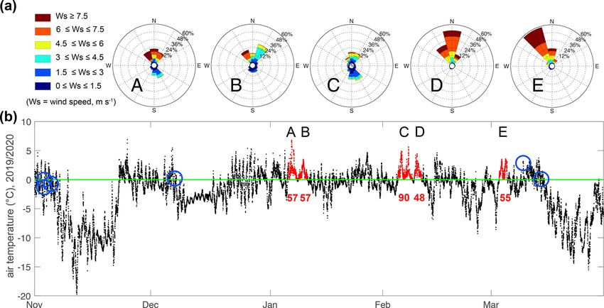
912                        A. F. Banwell et al.: 32-year record-high melt on the northern George VI Ice Shelf, Antarctica

on the northern GVIIS from all available cloud-free optical        > 1700 m a.s.l. were masked out so that melt over the ice
images from the Landsat 8 (2013 to 2020) and Sentinel-2            shelves was predominantly analysed and so that large to-
(2017 to 2020) satellites. Both our microwave-derived melt         pographic features (i.e. mountain peaks) in the radiometer’s
and optical image-derived surface ponding results are eval-        field of view were avoided.
uated alongside surface air temperature and wind data from            Based on radiative transfer simulations, radiometer bright-
the British Antarctic Survey (BAS) Fossil Bluff AWS (1979          ness temperatures at 19 GHz are typically sensitive to melt
to 2020) on the northwestern margin of the GVIIS (Fig. 1b,         down to a snow depth of ∼ 2 m (Picard et al., 2007; Leduc-
yellow star).                                                      Leballeur et al., 2020). Wet snow has a very high emissiv-
                                                                   ity compared to dry snow, but a flat surface of liquid water
3.1   Large-scale microwave radiometer observations of             has a low emissivity as well (Zwally, 1977). Therefore, at
      melt                                                         the transition from dry to wet snow, brightness temperatures
                                                                   increase quickly (i.e. indicating the presence of meltwater),
Microwave radiometer observations of melt, expressed as            but if melt intensifies, resulting in the formation of surface
brightness temperatures, depend primarily on the snow tem-         lakes, the brightness temperatures decrease. This effect has
perature profile and emissivity (Zwally, 1977). When liquid        been observed over sea ice when melt ponds are extensive
water exists in the snow, there is a significant increase in the   (e.g. Kern et al., 2020). Cautious interpretation of the “melt
absorption and therefore an increase in the microwave emis-        day” maps is therefore required, particularly if surface pond-
sivity, resulting in a higher brightness temperature. Large-       ing represents a large proportion of a grid cell’s total area.
scale melt information over the AP, including the GVIIS, was          For austral melt seasons from 1979/1980 to 2019/2020
derived from microwave radiometer (i.e. passive) observa-          (apart from 1987/1988 due to its missing data) and for
tions using the 1979 to 2020 near-daily 25 km melt product         each 25 km grid cell, we calculated the daily time series of
(version 2) of Picard et al. (2007) and Picard and Fily (2006),    microwave-radiometer-derived melt or no melt and the cu-
distributed on a polar stereographic grid. This melt or no-        mulative melt days each melt season (defined as 1 November
melt product, which has been used in several previous studies      to 31 March inclusive). This was done for both the whole
(e.g. Magand et al., 2008; Brucker et al., 2010; Wille et al.,     AP (i.e. extent of Fig. 1a) and for the northern GVIIS AOI
2019), is based on the algorithm of Torinesi et al. (2003) that    (Fig. 1b, red outline).
identifies the higher microwave brightness temperatures cor-
responding to melt using the radiation observed at 19 GHz in       3.2   Small-scale microwave scatterometer observations
horizontal polarization. If the observed brightness tempera-             of melt
ture on a given day exceeds an empirical threshold (defined
by the mean and variability of the brightness temperatures         For the northern GVIIS, we also derive smaller-scale melt in-
observed during the previous winter season, when melt did          formation from an enhanced resolution C-band (5.225 GHz)
not occur), the algorithm reports melt in the 25 km grid cell.     VV polarization radar backscatter image time series col-
Throughout this paper, we use the word “melt” when refer-          lected by EUMETSAT’s Advanced SCATterometer (AS-
ring to the presence of liquid meltwater (either in the near-      CAT), aboard the tandem polar-orbiting satellites MetOp-A
surface snow or on the surface) in the microwave data but          and MetOp-B. The 4.45 km enhanced product is obtained by
note that we are not referring to the process of active melt-      applying the Scatterometer Image Reconstruction (SIR) al-
ing; information that is that specific cannot be obtained from     gorithm with filtering (Lindsley and Long, 2016), which is
passive microwave data.                                            used to improve the spatial resolution of irregularly and over-
   The 1979 to 2020 brightness temperature time series was         sampled data (Early and Long, 2001). The effective spatial
acquired by five successive sensors. The Scanning Multi-           resolution was estimated at ∼ 12–15 km, three-fold finer than
channel Microwave Radiometer (SMMR), on the Nimbus 7               the effective resolution of the SMMR/SSMI-based product
satellite launched in late October 1978, collected data at         (∼ 50 km). For each day and for each grid cell, melt is as-
18 GHz (while the sensor operated every other day, daily av-       sumed to be present when the ASCAT signal is lower than
eraged brightness temperatures were used as input). Start-         the winter mean signal minus 3 dB, as proposed by Ashcraft
ing in 1987, the series of Special Sensor Microwave Imager         and Long (2006) using a melt model and QuikSCAT Ku-
(SSMI) sensors on the Department of Defense Meteorolog-            band (13.4 GHz) observations. Where snow and firn layers
ical Satellite Program (DMSP) platforms F8, F11, F13, and          are completely frozen, the C-band penetration depth is on
F17 collected data at 19 GHz. It is worth noting that there        the order of metres to tens of metres, but where snow and
was a significant data gap between 3 December 1987 and             firn layers have a high volumetric fractions of meltwater, the
14 January 1988, and therefore we do not include any data          penetration depth is likely to be up to tens of centimetres only
from this melt season in our analysis. Although the melt           (Weber Hoen and Zebker, 2000). As the penetration depth at
data are provided with a spatial resolution of 25 km, the ra-      5 GHz in dry snow and firn is larger than at 19 GHz, ASCAT
diometers’ 3 dB fields of view at 19 GHz are far larger (e.g.      C-band radar is likely to be more sensitive to melt at depth
69 km × 43 km for SSMI). Grid cells with surface elevations        than microwave radiometers at 19 GHz.

The Cryosphere, 15, 909–925, 2021                                                       https://doi.org/10.5194/tc-15-909-2021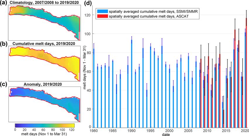
A. F. Banwell et al.: 32-year record-high melt on the northern George VI Ice Shelf, Antarctica                               913

   For austral melt seasons from 2007 to 2020, we calculate       ter in the water column to alter its optical properties, and
scatterometer-derived cumulative melt days for each 4.45 km       (3) there is minimal wind-induced surface roughness (Sneed
grid cell over our study AOI.                                     and Hamilton, 2007).
                                                                     All Landsat 8 and Sentinel-2 images acquired from
3.3   Landsat 8 and Sentinel-2 derived meltwater areas            1 November to 31 March each austral summer with a so-
      and volumes                                                 lar angle of > 15◦ , with ≥ 0.45 km2 water-covered pixels
                                                                  (equivalent to 500 Landsat pixels or 4500 Sentinel-2 pixels;
To calculate the time series of areal extents, depths, and        Moussavi et al., 2020) and which overlapped our study’s AOI
therefore total volumes of surface meltwater lakes on             (Fig. 1b, red outline) were analysed using the methods de-
the northern GVIIS for the seven austral summers from             scribed above. Once the images had been analysed, all tiles
2013/2014 to 2019/2020, we applied the threshold-based            with the same date were mosaicked together and then clipped
algorithm developed by Moussavi et al. (2020) to selected         to a mask of our AOI in the Geographic Information Sys-
multispectral imagery (see below) from Landsat 8 (30 m            tem package, QGIS v3.2. In total, for Landsat 8 we analysed
resolution, since 2013) and Sentinel-2 (10 m resolution,          mosaicked images for 191 dates from 6 December 2013 to
since 2017). Technical specifications for Landsat 8’s Oper-       12 March 2020, and for Sentinel-2 we analysed mosaicked
ational Land Imager data are available online from NASA           images for 14 dates from 3 January 2017 to 19 January 2020.
(https://landsat.gsfc.nasa.gov/operational-land-imager-oli/,      Of those images, nine Landsat 8 and Sentinel-2 image mo-
last access: 9 February 2021), and technical specifications for   saics had the same dates, and thus we merged those. First,
Sentinel-2’s MultiSpectral Instrument are available online        we resampled the Sentinel-2 data (10 m resolution) to the
from the ESA (https://sentinels.copernicus.eu/web/sentinel/       resolution of Landsat (30 m). Second, we kept overlapping
technical-guides/sentinel-2-msi, last access: 9 Febru-            water-covered pixels in preference to dry pixels and kept the
ary 2021). Analysis of pre-2013 optical imagery could             largest depths of the overlapping water-covered pixels. This
have been undertaken by tuning Moussavi et al.’s (2020)           resulted in a time series of 196 mosaicked images from 6 De-
threshold-based algorithm for the Landsat 7 Enhanced The-         cember 2013 to 12 March 2020 (Table S1 in the Supplement).
matic Mapper Plus (ETM+) sensor. However, significant             Errors and uncertainties associated with lake area and depth
data are missing since May 2003 due to the failure of the         retrieval methods for each sensor are thoroughly discussed in
scan line corrector (SLC) on ETM+ causing SLC-off gaps.           Moussavi et al. (2016, 2020), Pope et al. (2016), Williamson
Therefore, lake volumes derived from this sensor would            et al. (2018), and Fricker et al. (2020).
not be easily comparable to Landsat 8 and Sentinel-2 and             Due to temporally varying satellite paths and/or cloud
therefore would not necessarily extend the time series.           cover, only 11 out of the 196 mosaicked images covered the
   Moussavi et al.’s (2020) method, developed in parallel for     entirety of our AOI (Table S1 in the Supplement). Therefore,
Landsat 8 and Sentinel-2, combines separate threshold-based       to be able to compare areas and volumes of surface meltwa-
algorithms to detect (1) lakes, (2) rocks, and (3) clouds. Op-    ter on dates with incomplete AOI coverage, we first created a
timal thresholds for each band and band combination (e.g.         mask of all pixels that were wet on at least 1 of the 196 dates
Normalized Difference Water Index (NDWI), Normalized              analysed from 2013 to 2020 (Williamson et al., 2018), here-
Difference Snow Index (NDSI), and others) were determined         after called a “maximum wetted area mask”. Second, we cre-
by creating a training dataset based on selected Landsat 8 and    ated a “maximum volume mask” by assigning all wet pixels
Sentinel-2 images, which represented spectral properties of       in the maximum wetted area mask a depth equal to the max-
several classes (e.g. lakes, slush, snow, clouds, rocks, cloud    imum water depth observed out of all 196 images. Finally,
shadows). Most notably, to classify liquid-water-covered pix-     for each image mosaic with ≥ 10 % cloud-free coverage of
els, the NDWI is used (Pope et al., 2016; Bell et al., 2017)      our AOI (113 image dates), we normalized their total area
with NDWI thresholds of > 0.19 and > 0.18 for Landsat 8           and total volume of meltwater to our entire AOI using the
and Sentinel-2, respectively. Subsequently, to calculate the      following approaches. For each mosaicked image, we calcu-
water depths of those pixels determined to be water-covered,      lated the total observed meltwater area as a fraction of the
Moussavi et al. (2020) apply a physically based algorithm         total wetted area mask for the equivalent area. This fraction
that has more commonly been applied in Greenland (Sneed           was then multiplied by the total area of the maximum wetted
and Hamilton, 2007; Banwell et al., 2014; Pope et al., 2016;      area mask over the whole AOI. To normalize the meltwa-
Williamson et al., 2018) and more recently in Antarctica          ter volume to the AOI, we did the same but instead used the
(Bell et al., 2017; Dell et al., 2020; Arthur et al., 2020b).     maximum volume mask.
This algorithm calculates lake water depth using the rate
that sunlight passing through a water column is attenuated        3.4   Local weather station data
with depth, lake-bottom albedo, and optically deep water re-
flectance (Philpot, 1989). This approach makes a number of        We analyse the only available local AWS data in order to
assumptions, including that (1) the lake bottom has a ho-         investigate the possible atmospheric driver(s) of the excep-
mogenous albedo, (2) there is little to no particulate mat-       tional melt event over the northern GVIIS in 2019/2020.

https://doi.org/10.5194/tc-15-909-2021                                                    The Cryosphere, 15, 909–925, 2021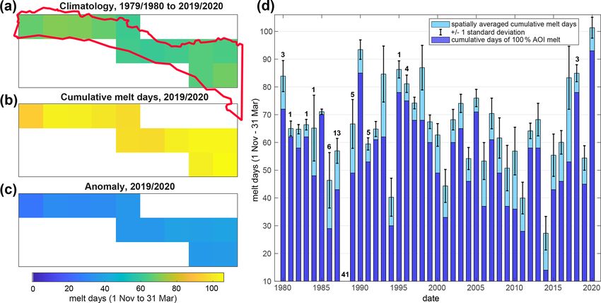
914 A. F. Banwell et al.: 32-year record-high melt on the northern George VI Ice Shelf, Antarctica
Near-surface (2 m) temperature, relative humidity, wind di- 4 Results
rection, and wind speed data are available from the BAS Fos-
sil Bluff AWS (Fig. 1b, yellow star, location: −71.329◦ S, 4.1 Microwave-radiometer-derived melt observations
−68.267◦ W, 66 m a.s.l.), at 12 h intervals from 1979 to 1999 over the Antarctic Peninsula
and at 5 or 10 min intervals from 2000 to 2020. However, sig-
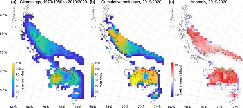
nificant data gaps are present between 2000 and early 2007. For the AP, cumulative melt days in the 2019/2020 austral
First, we compare the 2019/2020 daily mean air temper- melt season are highest in the southwestern areas of the AP
atures with the daily mean temperatures from 1979 to 2020 (including the Wilkins and George VI ice shelves), in addi-
(using 12 h data at noon and midnight local time), i.e. the tion to the northern area of the Larsen C Ice Shelf (Fig. 2b).
complete time period for which we also have microwave In comparison, cumulative melt days in 2019/2020 are rel-
radiometer data. Second, for 2007 to 2020, which is when atively low over the southern areas of the Larsen C. The
AWS data are available at a higher frequency and data gaps spatially averaged cumulative melt days in the 2019/2020
are minimal (6 months in the total record were missing val- melt season over the entire AP amount to 47 d (Fig. 2b),
ues, but these were < 15 % of the expected total for each which is 53 % higher (Fig. 2c) than the spatially averaged
of those months), we use the 10 min data to calculate the climatology from 1979/1980 to 2019/2020 (31 d; Fig. 2a).
length of time (in hours) when surface air temperatures are However, of these 41 melt seasons, the 1992/1993 melt sea-
continuously ≥ 0 ◦ C during each melt season. Although the son has the most spatially averaged cumulative melt days
air temperature measured at a height of 2 m by the AWS will over the AP (62 d; Fig. S1 in the Supplement). During the
vary slightly from that at the ice surface, for the purposes 1992/1993 season, although cumulative melt days over the
of this study, we assume these temperatures to be equiva- northern GVIIS were only slightly higher than the 1979/1980
lent (Kuipers Munneke et al., 2012). We also consider the to 2019/2020 mean (Fig. S1d), the cumulative melt days on
occurrence of foehn winds, which are warm, dry winds of- the Larsen C Ice Shelf were particularly high, with a max-
ten produced on the leeward side of mountains (Cape et imum of 117 cumulative melt days in the southern area of
al., 2015) and commonly occur on the AP (Luckman et al., this ice shelf (Fig. S1c). This finding is contrary to the re-
2014; Elvidge et al., 2016). Over GVIIS, the steep topog- sults of Bevan et al. (2020), who report that Larsen C expe-
raphy that generates foehn flow is provided by Alexander rienced a 41-year record-high melt year in 2019/2020. Be-
Island. We analyse foehn wind occurrence using a modi- van et al.’s (2020) results are based on microwave radiometer
fied version of a metric previously used over the Larsen (SMMR/SSMI) data for melt seasons from 1979/1980 un-
C Ice Shelf (Wiesenekker et al., 2018; Datta et al., 2019), til 2016/2017, followed by microwave scatterometer (AS-
whereby a “foehn condition” is considered to initiate when CAT) data from 2017/2018 to 2019/2020. In contrast, we
air temperatures increase by ≥ 1 ◦ C, wind speed increases use SMMR/SSMI data over the AP for the full 1979 to 2020
by ≥ 1.5 m s−1 , and relative humidity decreases by ≥ 5 %, period to preserve consistency. As we explain in Sect. 3.2,
all relative to the previous time step. We use a wind speed ASCAT C-band radar is likely to be more sensitive to melt
threshold of 1.5 m s−1 instead of the higher threshold of at depth than microwave radiometers, thus resulting in Be-
3.5 m s−1 used by Datta et al. (2019) for the Cabinet Inlet van et al.’s (2020) higher calculated melt over Larsen C in
AWS to account for lower foehn wind speeds over the north- the 2019/2020 season when combining data sources into one
ern GVIIS, which result from the lower mean elevation of time series.
the mountains on Alexander Island compared to those on the
AP west of Cabinet Inlet (van Wessem et al., 2015). This 4.2 Microwave-derived melt observations over the
foehn condition is assumed to remain until the conditions northern GVIIS
(with respect to the period preceding the foehn condition)
are no longer met. Finally, we also examine differences in at- Over the northern GVIIS, microwave-radiometer-derived
mospheric regimes (temperature, wind direction and speed) spatially averaged cumulative melt days over the study AOI
within each wind direction class (northeasterly, northwest- (12 grid cells, total area = 7556 km2 ) in the 2019/2020 aus-
erly, southeasterly, and southwesterly). tral melt season amount to 101 d (Fig. 3b and d), which is
We note that it is beyond the scope of this study for us to higher than for any other melt season since the record began
identify specific mesoscale drivers of this exceptional melt in 1979/1980 and is 53 % higher (Fig. 3c) than the spatially
event, especially as 2019/2020 is not a record melt season averaged climatology (66 melt days) from 1979/1980 to
for the AP as a whole (see Sect. 4.1), and regional climate 2019/2020 (Figs. 3 and S2). However, as 41 d of microwave
models frequently struggle to resolve localized surface melt radiometer data for the 1987/1988 season are missing, we
in regions with highly variable topography (Van Wessem et only conclude that 2019/2020 was the most significant melt
al., 2015; Barrand et al., 2013), such as is the case for the season over 32 years (Fig. 3d). This result is supported by
GVIIS and its surrounding higher terrain. the analysis of scatterometer-derived melt data from ASCAT,
which show that the number of spatially averaged cumula-
tive melt days over the study AOI in the 2019/2020 austral
The Cryosphere, 15, 909–925, 2021 https://doi.org/10.5194/tc-15-909-2021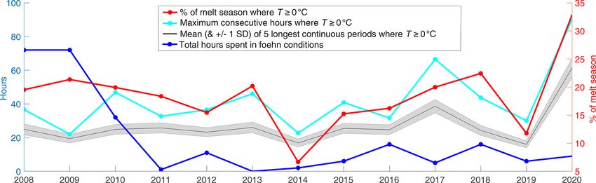
A. F. Banwell et al.: 32-year record-high melt on the northern George VI Ice Shelf, Antarctica 915
Figure 2. Microwave-radiometer-derived maps of surface and near-surface melt days over the AP: (a) the climatology (i.e. mean cumulative
melt days per season) from 1979/1980 to 2019/2020 (excluding 1987/1988 due to missing data), (b) cumulative melt days in 2019/2020, and
(c) the 2019/2020 melt season anomaly (i.e. b minus a). Melt days are counted within the period 1 November to 31 March (inclusive) each
austral summer. The location of the study AOI is shown by a red outline in (a) and (b) and as a green outline in (c). The black outline of the
AP is from the MODIS Mosaic of Antarctica (Haran et al., 2014).
melt season was 117 d, which is 70 % higher than the spa- longer continuous period (91 d) relative to any other year in
tially averaged climatology (69 melt days) from 2007/2008 this record.
to 2019/2020 (Fig. 4). The microwave-radiometer-derived Since addressing uncertainties associated with microwave
data suggests that 1989/1990 has the second highest num- data products of binary melt–no melt information is challeng-
ber of spatially averaged cumulative melt days (93) over the ing, this study uses two distinct microwave remote sensing
study AOI (Figs. 3d and S2). techniques and algorithms to build further confidence in our
Using the microwave radiometer data to consider the cu- conclusion. Moreover, our analysis of the sensitivity of the
mulative days of melting occurring over 100 % of the AOI microwave radiometer (Fig. S4) and scatterometer (Fig. S5)
each season, 2019/2020 also sees the highest such number of melt detection algorithms to decreasing or increasing their
days (93; see Fig. 3d, dark blue bars), and 1989/1990 sees threshold values shows that the 2019/2020 melt season re-
the second highest number of days (85). These values can be mains exceptional and that it is a 32-year record.
compared to a mean value of 53 cumulative melt days over
100 % of the AOI from 1979/1980 to 2019/2020. Note that 4.3 Optical image-derived meltwater areas and
for each season, we do not specifically consider the mean volumes over the northern GVIIS
areal extent of melting as this variable is found to be almost
directly proportional (r 2 = 0.9973) to the spatially averaged From 2013 to 2020, when we have Landsat 8 and/or Sentinel-
cumulative melt days (Fig. S3). 2 optical imagery available, the day with the maximum ob-
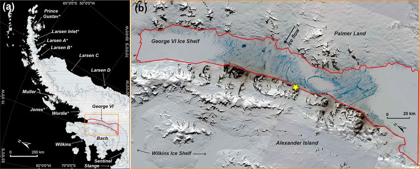
In terms of intra-annual patterns in percentage melt area served area (1.2 × 10⁹ m2 ) and volume (6.2 × 10⁸ m3 ) of
over the northern GVIIS in 2019/2020, the microwave ra- ponded surface meltwater on the northern GVIIS is 19 Jan-
diometer data shows that 100 % of the AOI area experiences uary 2020 (Figs. 1b, 5b, S6 and S7, Table S1), when 23 % of
melting every day from 24 November 2019 to 22 Febru- the AOI is covered in ponded water. On this date, it is for-
ary 2020 (Fig. 5c). After 22 February, the area of melting tuitous that the whole of our AOI is visible in a mosaic of
drops to 0 % of the AOI over just 3 d, which is consistent cloud-free Sentinel-2 image scenes (Fig. 1b; background im-
with a drop in the mean daily air temperature (Fig. 5a). For age) and is also fully visible in a mosaic of Landsat 8 images
a few weeks after 25 February, the area of melting fluctu- acquired on 17 and 19 January (not shown). Calculated areas
ates significantly, consistent with the air temperature fluctu- and depths of meltwater lakes on 19 January 2020 over the
ating around 0 ◦ C. On 6 and 7 March 2020, 100 % of the entire AOI are shown in Fig. S6. The mean depth of all water-
AOI is observed to melt again. From 16 March 2020, no ad- covered pixels on this date is 0.52 m, and the maximum depth
ditional melting is observed. Compared to the mean melt area is 3.9 m. Unlike on other dates with much cloudier imagery,
over the two time periods shown in Fig. 5c (i.e. 1979/1980 to normalization of meltwater areas and volumes to the AOI on
2019/2020 and 2013/2014 to 2019/2020), the observed melt 19 January 2020 is not required (see Sect. 3.3 for method de-
area in 2019/2020 covers 100 % of the AOI for a significantly tails, Fig. S7 for plots of both the observed and normalized
meltwater areas and volumes for the 2013/2014 to 2019/2020
https://doi.org/10.5194/tc-15-909-2021 The Cryosphere, 15, 909–925, 2021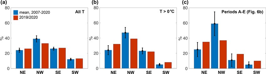
916                          A. F. Banwell et al.: 32-year record-high melt on the northern George VI Ice Shelf, Antarctica

Figure 3. Microwave-radiometer-derived cumulative melt days over the northern GVIIS AOI (see Fig. 1b for location, red outline) from
1 November to 31 March. (a–c) Maps of surface and near-surface melt days per 25 km grid cell. The relative location and shape of the
study’s AOI is shown by the red outline. White cells are out of the AOI. (a) Mean cumulative melt days for each 25 km grid cell for austral
summers from 1979/1980 to 2019/2020, apart from 1987/1988 due to data unavailability. (b) Cumulative melt days per grid cell in the
2019/2020 austral summer. (c) Anomaly of the 2019/2020 melt season (i.e. b minus a). (d) Light blue bars represent spatially averaged (i.e.
over the 12 grid cells in the AOI) cumulative melt days for each austral summer from 1979/1980 to 2019/2020 (apart from 1987/1988). The
x axis dates indicate the second year of each austral summer, e.g. 2020 corresponds to the 2019/2020 season. Black error bars show ± 1
standard deviation from the spatially averaged cumulative melt days. Dark blue bars show cumulative days when the melt extent is 100 %
of the AOI for each summer from 1979/1980 to 2019/2020. For melt seasons with missing data, the total number of missing data days is
indicated by the black number above the corresponding bar.

Figure 4. (a–c) Active microwave-derived (i.e. ASCAT) cumulative melt days over the northern GVIIS AOI (see Fig. 1b for location, red
outline), relative to the passive microwave time series (Fig. 3a–c). (a) Mean cumulative melt days for austral summers from 2007/2008
to 2019/2020. (b) Cumulative melt days in the 2019/2020 austral summer. (c) Anomaly of the 2019/2020 melt season (i.e. b minus a).
(d) Red bars represent microwave scatterometer-derived, spatially averaged (i.e. over the AOI) cumulative melt days for austral summers
from 1979/1980 to 2019/2020, with red error bars showing ± 1 standard deviation from the mean. Blue bars show microwave-radiometer-
derived, spatially averaged cumulative days from 1979/1980 to 2019/2020, with blue error bars showing ± 1 standard deviation from the
mean. The x axis dates indicate the second year of each austral summer, e.g. 2020 = 2019/2020.

The Cryosphere, 15, 909–925, 2021                                                             https://doi.org/10.5194/tc-15-909-2021
A. F. Banwell et al.: 32-year record-high melt on the northern George VI Ice Shelf, Antarctica                                          917

Figure 5. (a) Surface (2 m) air temperature data from the Fossil Bluff AWS (location in Fig. 1b, yellow star). The daily mean air temperature
for the 2019/2020 melt season is shown by the red line, daily mean temperatures for the seven melt seasons from 2013/2014 to 2019/2020
are shown by the blue line, ± 1 standard deviation from that blue line is shown by the areas of blue shading, and the daily mean temperature
from 1979 to 2020 (using 12 h data) is shown by the green line. The horizontal dashed black line depicts 0 ◦ C. (b) Calculated volumes of
surface meltwater ponding in the GVIIS AOI from 2013/2014 to 2019/2020 derived from Landsat 8 and Sentinel-2 optical imagery. Data
from mosaicked images are only plotted if the image includes > 10 % of the study’s AOI (Fig. 1, red outline) that is cloud free; data from
mosaicked images on 113 images total are shown. On dates when imagery does not cover 100 % of the AOI, observed meltwater volumes
are normalized to the AOI (see Sect. 3.3 for further details and Fig. S7 for a plot of all the observed meltwater volumes). (c) Microwave-
radiometer-derived near-surface melt extent over the GVIIS AOI (Fig. 1b, red outline) as a % of the total area (7556 km2 ). Daily areas of
melting for 2019/2020 are shown by the red line, the daily mean area of melting from 2013/2014 to 2019/2020 is shown by the dark blue
line, and the daily mean area of melting from 1979/1980 to 2019/2020 (excluding 1987/1988) is shown by the light blue line.

https://doi.org/10.5194/tc-15-909-2021                                                             The Cryosphere, 15, 909–925, 2021
918                        A. F. Banwell et al.: 32-year record-high melt on the northern George VI Ice Shelf, Antarctica

melt seasons, and Table S1 for details of all optical imagery     ten more than 1 standard deviation greater than the multi-
analysed).                                                        year daily mean (Fig. 5a). Considering all recorded temper-
   In all the seven melt seasons analysed with optical im-        ature data in each melt season from 2007 to 2020, a higher
agery, ponded surface meltwater volumes do not peak un-           percentage (33 %) of 2019/2020 has air temperatures ≥ 0 ◦ C
til January or February (Fig. 5b). However, in 2019/2020,         compared to any prior season (Fig. 6, red line).
meltwater volumes start to increase rapidly in late Decem-           We also examine the potential role of foehn winds on
ber/early January, which is earlier than in any other season,     driving melt in 2019/2020. Foehn conditions (as described
and corresponds with above-average air temperatures in late       in Sect. 3.4) are only present for about 9 h over the entire
December 2020 (Fig. 5a, also see Sect. 4.4 for analysis of        2019/2020 season (Fig. 6, blue line), and occur in early and
local weather conditions). In 2019/2020, volumes of melt-         late summer (Fig. 7b, blue circles) when winds are typically
water ponding are highest in early January and then again in      stronger. We also note that the total time during each sea-
early February; corresponding with periods when mean daily        son when foehn conditions are calculated from AWS data
air temperatures are ≥ 0 ◦ C for extended periods (Fig. 5a).      has been relatively low since the 2007/2008 and 2008/2009
There is a notable decrease in surface meltwater ponding          melt seasons, which each had a total of about 72 h of foehn
volume in mid to late January 2020 during a period of sub-        flow (Fig. 6). Therefore, foehn conditions do not appear to be
stantially colder air temperatures (i.e. < 0 ◦ C, Fig. 5a) that   dominant in driving melt in the 2019/2020 season.
likely resulted in widespread refreezing of surface meltwater        Finally, we analyse the potential role of warm air advec-
(Fig. 5b).                                                        tion, resulting in sensible heat transport, on the high melt in
   The second largest melt season in terms of meltwater           2019/2020. Considering wind direction alongside air tem-
ponding is 2017/2018, with a peak in total meltwater area         perature for melt seasons from 2007 to 2020, the climatol-
(4.6×10⁸ m2 ) and volume (2.5×10⁸ m3 ) on 29 January 2018         ogy indicates that northwesterly winds dominate flow at all
(Figs. 5b and S7). However, these two values are less than        temperatures (Fig. 8a) but are more dominant when temper-
half of the respective values measured on 19 January 2020.        atures are ≥ 0 ◦ C (Fig. 8b) and are even more so when we
Aside from 2019/2020 and 2017/2018 (i.e. the melt seasons         limit analysis to just the five longest periods of sustained
with the greatest and second greatest volumes of surface          temperatures ≥ 0 ◦ C in each season (Fig. 8c). However, in
ponding, respectively), the other five melt seasons have rela-    the 2019/2020 season, northwesterly winds are less domi-
tively low volumes of ponded meltwater.                           nant (33 % vs. 39 %; Fig. 8a), especially when only temper-
                                                                  atures ≥ 0 ◦ C are considered (39 % vs. 47 %; Fig. 8b), and
4.4   Near-surface atmospheric conditions                         are further limited when only the five longest periods of sus-
                                                                  tained temperatures ≥ 0 ◦ C (Fig. 7; periods A–E) are consid-
Analysis of the mean daily surface air temperatures (derived      ered (37 % vs. 59 %; Fig. 8c). Instead, the proportion of wind
from 12 h values) from the Fossil Bluff AWS from 1979 to          coming from the northeast is higher in 2019/2020 compared
2020 indicates that 2019/2020 is anomalously warm over five       to the climatology (26 % vs. 24 %; Fig. 8a), particularly when
multi-day periods starting in late November (Figs. 5a and         temperatures are ≥ 0 ◦ C (32 % vs. 24 %, Fig. 8b).
S8). During these periods, mean daily air temperatures are           The 2007 to 2020 climatology shows that (as expected)
≥ 0 ◦ C for sustained time periods of up to a week. The total     northwesterly winds typically include a higher proportion of
number of positive degree days for the 2019/2020 melt sea-        warmer, faster winds, than other wind directions (Fig. S9a),
son (1 November to 31 March inclusive) is 40, compared to         whereas northeasterly winds are typically lower speed over-
19 ± 14 d (mean ± 1 standard deviation) from 1979/1980 to         all and are generally colder (Fig. S9b). However, in the
2019/2020.                                                        2019/2020 melt season, we show that both northwesterly and
   We also analyse the high-resolution (10 min) AWS data          northeasterly winds are warmer at lower wind speeds. There-
from 2007 to 2020 to identify periods of sustained high           fore, having eliminated foehn flow as a significant driver for
temperatures, when it is possible that no refreezing at all       surface melt in this season, we suggest that the increased ad-
occurred during the diurnal cycles, potentially enhancing         vection of warm air from both the northwest and northeast
the surface melt–albedo feedback effect. We find that the         contributed to the sustained warm air temperatures we ob-
longest continuous period when air temperatures are ≥ 0 ◦ C       serve.
in 2019/2020 is 90 h in early February (Fig. 6, cyan line,
and Fig. 7, label C). The longest five such time periods in
2019/2020 are labelled A to E in Fig. 7, and it is notable that
two pairs of periods, A and B and C and D, are only sep-
arated by a matter of hours. The mean length of these five
longest periods when temperatures ≥ 0 ◦ C in 2019/2020 is
61 h, which is longer than for any other season in the 2007
to 2020 high-resolution AWS record (Fig. 6, black line). We
also note that the temperature during these five periods is of-

The Cryosphere, 15, 909–925, 2021                                                     https://doi.org/10.5194/tc-15-909-2021
A. F. Banwell et al.: 32-year record-high melt on the northern George VI Ice Shelf, Antarctica 919
Figure 6. Analysis of sustained warm (≥ 0 ◦ C) air temperature (T ) periods and foehn wind occurrence for the 2007/2008 to 2019/2020 melt
seasons. The cyan line shows the maximum number of consecutive hours in each melt season when T ≥ 0 ◦ C. The black line shows the
mean length (hours) of the five longest periods when T ≥ 0 ◦ C for each season, with the grey shading indicating ±1 standard deviation from
that mean. The red line shows the proportion of each season (1 November to 31 March) when T is ≥ 0 ◦ C. The blue line shows the total
number of hours spent in a foehn condition (see Sect. 3.4 for definition) each season. The x axis dates indicate the second year of each austral
summer, e.g. 2020 corresponds to the 2019/2020 season.
Figure 7. The 2019/2020 wind and air temperature and data (10 min) from the Fossil Bluff AWS. (a) Wind roses for corresponding periods
of sustained air temperatures (A–E) indicated in (b). (b) Air temperature record for 2019/2020 with the five longest periods of temperatures
≥ 0 ◦ C shown in red. The red numbers below these time periods indicate the total number of hours when the temperature is continuously
≥ 0 ◦ C. It is notable that only 9 h separates periods A and B and only 14 h separates C and D. The six blue circles indicate periods when we
calculate foehn conditions to be present (see Sect. 3.4 for methods).
5 Discussion and/or wetness of the subsurface snow and firn (see Sect. 3.1
for more detail). Therefore, we cannot directly compare the
5.1 Comparison of the optical image and microwave-derived melt data with the optical image-derived
microwave-derived melt data over the northern ponding data. However, together these data provide informa-
GVIIS, 2013 to 2020 tion on the time between melt onset and surface ponding over
the northern GVIIS, and likewise the disappearance of sur-
Microwave melt data are binary (i.e. the algorithm indicates face ponding and melt termination at the end of the season.
there is either melt or no melt); thus, these data do not mea- For the time period from 2013/2014 to 2019/2020, when
sure the intensity of the melting nor the volume of meltwa- we have three independent datasets, 2019/2020 was anoma-
ter present. Additionally, while the optical data are used to lous for the following reasons. Optical imagery indicates this
detect the presence of surface meltwater, the microwave ra- season had the largest volumes of observed surface meltwater
diometer data can contain melt information through a snow ponding (Fig. 5b), microwave radiometer- and scatterometer-
depth of < 2 m, depending on the presence of surface lakes
https://doi.org/10.5194/tc-15-909-2021 The Cryosphere, 15, 909–925, 2021920 A. F. Banwell et al.: 32-year record-high melt on the northern George VI Ice Shelf, Antarctica
Figure 8. Percentage (%) of wind each season (1 November to 31 March) at Fossil Bluff AWS that is northeasterly (NE), northwesterly
(NW), southeasterly (SE), and southwesterly (SW), with the interannual (2007/2008 to 2019/2020) mean shown in blue and the 2019/2020
values shown in red. (a) Wind direction proportions using all recorded air temperatures. (b) Wind direction proportions only when recorded
temperatures are ≥ 0 ◦ C. (c) Wind direction proportions only during the five longest periods of T ≥ 0 ◦ C (A to E, Fig. 7b) for all melt seasons
(blue) and for 2019/2020 (red).
derived data show that it also had the most spatially extensive AOI) for the greatest number days (Fig. 5c), and the great-
melt (i.e. 100 % of the AOI) for the greatest number of days est number of cumulative melt days (Figs. 3 and S2); re-
(Fig. 5c), as well as the highest number of cumulative melt sults that are corroborated by our scatterometer-derived melt
days (Figs. 3d, 4d and S2). data from 2007 to 2020 (Fig. 4). As mentioned in Sect. 3.2,
In the 2019/2020 season, the microwave radiometer data scatterometer-derived cumulative melt days (117 d) are likely
first indicate the presence of surface and near-surface melt higher than those derived from the radiometer data (101 d;
on 22 November, which extends to over 100 % of the AOI by Fig. 4d) because C-band radiation has a larger penetration
24 November (Fig. 5c). However, surface meltwater ponding depth and thus likely detect melt at greater depths (Weber
is not observed in the (non-continuous, both due to acquisi- Hoen and Zebker, 2000).
tion coverage and cloud coverage) optical imagery until mid- The microwave radiometer data suggest a slightly negative
December (Fig. 5b). This offset in the timing of the observa- trend in cumulative melt days and areal melt extent (Figs. 2,
tions is likely due to the fact that although sustained positive 3d and S2) from the mid-1990s until ∼ 2015/2016, which is
air temperatures in late November 2020 increased surface consistent with negative near-surface air temperature trends
and near-surface melt rates, it takes time for surface ponds over the AP until 2016, likely relating to oscillations in the
to develop in the early melt season, and this will only happen Southern Annular Mode (SAM) (Picard et al., 2007; Turner
once suitable surface and firn and ice conditions are present. et al., 2016). This temperature trend is in contrast to the years
However, once surface ponds have developed, this offset in prior to the mid to late 1990s, when trends over the AP from
the timing between warm temperatures and ponding is much available research station AWSs had generally been positive
less apparent. For example, sustained warm temperatures in since the 1950s (Turner et al., 2005) (though this is not ap-
early January (Fig. 7b, periods A and B) and early Febru- parent in our microwave-radiometer-derived melt data).
ary (Fig. 7b, periods C and D) coincide with periods when
surface meltwater volumes derived from optical imagery are 5.3 Local climatic controls of the 2019/2020 melt event
relatively high (Fig. 5b). Towards the end of the melt sea-
son, although there are no cloud-free Landsat 8 or Sentinel- Our air temperature analysis using both daily means (from
2 images available after mid-February 2020 (Fig. 5b), our 1979; Fig. S8), and higher temporal resolution (10 min)
visual analysis of Terra and Aqua MODIS optical imagery data (from 2007; Fig. 7b) shows anomalously long time pe-
suggests that open-water lakes remain until at least 25 Febru- riods when air temperatures were continuously ≥ 0 ◦ C in
ary, with some lakes potentially remaining until mid to late 2019/2020. Using the 10 min data, the longest such period
March. Meanwhile, the microwave-radiometer-derived melt was 90 h in 2019/2020, suggesting that no refreezing oc-
drops to zero by 25 February but then fluctuates until mid- curred during that time (Fig. 7b). Overall, 2019/2020 also
March (Fig. 5c); perhaps indicative of a melt–refreeze pro- had the highest proportion of an entire season (33 %) when
cess. temperatures were ≥ 0 ◦ C (Fig. 6). We suggest that the sus-
tained periods of warm temperatures, which started unusu-
5.2 Near-surface and surface melting over the northern ally early in the melt season, both initiated and enhanced
GVIIS, 1979 to 2020 melting in 2019/2020. The presence of just a small quantity
of surface meltwater early in the melt season is especially
From 1979/1980 to 2019/2020 (excluding the 1987/1988 important as this will have a disproportionate effect on over-
season), the microwave radiometer data show that 2019/2020 all surface melt production due the non-linear melt–albedo
was the largest melt season over the northern GVIIS in feedback process (Trusel et al., 2015).
terms of the most spatially extensive melt (i.e. 100 % of the
The Cryosphere, 15, 909–925, 2021 https://doi.org/10.5194/tc-15-909-2021A. F. Banwell et al.: 32-year record-high melt on the northern George VI Ice Shelf, Antarctica 921
Compared to the 2007 to 2020 AWS record, the 2019/2020 ber) likely contributed to the exceptional 2019/2020 melt
austral summer experienced a lower proportion of northwest- event. These periods of sustained warm temperatures were
erly wind (Fig. 8), though these winds are warmer at lower likely driven by sensible heat transported by warm north-
speeds (Fig. S9a). Instead, the proportion of northeasterly westerly and northeasterly low-speed winds. Consistent with
wind was higher in 2019/2020 compared to the 2007 to 2020 our finding that the proportion of northwesterly wind de-
climatology (Fig. 8), and these winds were also warmer at creased in 2019/2020 compared to the 2007 to 2020 period,
lower speeds (Fig. S9b). We therefore suggest that sensible we only calculate a total of ∼ 9 h of foehn conditions for this
heat transported by warm, lower-speed, northwesterly and season, which occurred in early and late summer. It is there-
northeasterly wind helped to drive melting in 2019/2020. We fore notable that although the high melt event over the north-
also note that a record high Indian Ocean Dipole (IOD) in ern GVIIS is 2019/2020 was caused by warmer than aver-
the early part of the 2019/2020 melt season is discussed in age air temperatures, such local weather conditions were not
Bevan et al. (2020) as a potential large-scale driver for warm, foehn-driven.
northerly surface winds on the western AP. However, as the Using Landsat 8 and Sentinel-2 satellite imagery, we
Fossil Bluff AWS does not measure radiation, we cannot observed the maximum volume of meltwater ponding on
exclude the possibility that the high melt in the 2019/2020 the northern GVIIS (7850 km2 ) on 19 January 2020, when
was not partially attributable to enhanced longwave radia- ∼ 23 % of this area was covered in surface lakes with a mean
tion (potentially resulting from cloud cover) and/or increased depth of 0.5 m. In comparison, only 10 % of the 3200 km2
shortwave radiation (potentially resulting from an absence of area of the Larsen B Ice Shelf that disintegrated in 2002
cloud cover). was covered in surface ponds with a mean depth of 0.8 m
Although warm foehn winds are known to initiate peri- (Banwell et al., 2014). However, unlike the relatively uncon-
ods of sustained melt and/or produce firn densification due strained and therefore extensional ice flow of the Larsen B
to near surface melt and refreezing (Luckman et al., 2014), Ice Shelf (e.g. MacAyeal et al., 2003; Scambos et al., 2004),
our analysis suggests that the 2019/2020 melt season experi- GVIIS has dominantly compressive flow, enabling the shelf
enced limited foehn conditions (see Sect. 3.4) in the early to remain relatively stable despite large volumes of surface
(and then late) melt season (Fig. 7b). This timing is pre- water (Lai et al., 2020). Despite this, our results show that
dictable foehn flow behaviour; e.g. over the Larsen C, foehn some of the areas of dense surface ponding near the east-
winds are strongest in winter, when wind speeds are gener- ern margin of the northern GVIIS coincide with areas clas-
ally higher (Wiesenekker et al., 2018; Datta et al., 2019). Our sified as vulnerable to hydrofracture by Lai et al. (2020,
observation of minimal foehn wind conditions over the north- their Fig. 4), particularly if pre-existing surface crevasses are
ern GVIIS in 2019/2020 is consistent with our observation of present. Though individual years of exceptional high surface
an overall decrease in the frequency of northwesterly winds melt do work to decrease ice shelf stability, further research
(Fig. 8), which are typically responsible for foehn flow. As is required to better constrain the potential timing and style
we do not find 2019/2020 to be a record melt season for the of a GVIIS collapse event due to the competing controlling
AP as a whole (see Sect. 4.1), we chose to focus on identify- factors of surface melt, basal melt, and stress regime.
ing local climate drivers of this exceptional melt event based
on the observational record, rather than trying to establish
large-scale atmospheric drivers. Code and data availability. The code used to calculate ar-
eas and volumes of surface meltwater is available at
https://github.com/mmoussavi/Lake_Detection_Satellite_Imagery/
(Moussavi, 2020a) and described in detail in Moussavi et al. (2020).
6 Conclusions
A comprehensive dataset of Antarctic lakes from Landsat 8 im-
agery is available at https://doi.org/10.15784/601401 (Moussavi,
We have used microwave radiometer data from 1979 to 2020 2020b). The passive microwave melt product is available at
and microwave scatterometer data from 2007 to 2020 to show http://pp.ige-grenoble.fr/pageperso/picardgh/melting/ (last access:
that the 2019/2020 austral melt season on the northern GVIIS 1 October 2020). The ASCAT enhanced resolution product is avail-
was exceptional in terms of both cumulative melt days and able at https://www.scp.byu.edu/data/Ascat/SIR/msfa/Ant.html
areal extent compared to the previous 31 melt seasons since (last access: 1 October 2020). Temperature data are available from
1988/1989 and possibly since the beginning of the record the BAS Fossil Bluff AWS at 10 min intervals from 2006 to 2020
in 1979/1980. We also used multi-spectral satellite imagery (https://legacy.bas.ac.uk/cgi-bin/metdb-form-2.pl?tabletouse=U_
from 2013 to 2020 to show that the observed surface meltwa- MET.FOSSIL_BLUFF_ARGOS&complex=1&idmask=.....&acct=
ter ponding on the northern GVIIS in 2019/2020 was also ex- u_met&pass=weather, last access: 1 October 2020), and at intervals
ceptional in areal extent and estimated volume since at least ranging from 12 to 1 h from 1979 to 2006 (https://legacy.bas.ac.uk/
cgi-bin/metdb-form-2.pl?tabletouse=U_MET.FOSSIL_BLUFF_
2013/2014.
SYNOP&complex=1&idmask=.....&acct=u_met&pass=weather,
Our analysis, based on the local weather data from the last access: 1 October 2020). The U.S. National Ice Center
Fossil Bluff AWS, shows that sustained periods of warm Operational Antarctic Ice Front and Coastline Data Set is available
(≥ 0 ◦ C) temperatures from early in the season (late Novem-
https://doi.org/10.5194/tc-15-909-2021 The Cryosphere, 15, 909–925, 2021You can also read