Mobile monitoring of urban air quality at high spatial resolution by low-cost sensors: impacts of COVID-19 pandemic lockdown - Recent
←
→
Page content transcription
If your browser does not render page correctly, please read the page content below
Atmos. Chem. Phys., 21, 7199–7215, 2021
https://doi.org/10.5194/acp-21-7199-2021
© Author(s) 2021. This work is distributed under
the Creative Commons Attribution 4.0 License.

Mobile monitoring of urban air quality at high spatial resolution by
low-cost sensors: impacts of COVID-19 pandemic lockdown
Shibao Wang1 , Yun Ma1 , Zhongrui Wang1 , Lei Wang1 , Xuguang Chi1 , Aijun Ding1 , Mingzhi Yao2 , Yunpeng Li2 ,
Qilin Li2 , Mengxian Wu3 , Ling Zhang3 , Yongle Xiao3 , and Yanxu Zhang1
1 School of Atmospheric Sciences, Nanjing University, Nanjing, China
2 BeijingSPC Environment Protection Tech Company Ltd., Beijing, China
3 Hebei Sailhero Environmental Protection Hi-tech. Ltd., Shijiazhuang, Hebei, China

Correspondence: Yanxu Zhang (zhangyx@nju.edu.cn)

Received: 9 November 2020 – Discussion started: 24 November 2020
Revised: 8 April 2021 – Accepted: 8 April 2021 – Published: 11 May 2021

Abstract. The development of low-cost sensors and novel           tion, accurate traceability, and potential mitigation strategies
calibration algorithms provides new hints to complement           at the urban micro-scale.
conventional ground-based observation sites to evaluate the
spatial and temporal distribution of pollutants on hyper-
local scales (tens of meters). Here we use sensors deployed
on a taxi fleet to explore the air quality in the road net-       1   Introduction
work of Nanjing over the course of a year (October 2019–
September 2020). Based on GIS technology, we develop a            Urban air pollution poses a serious health threat with > 80 %
grid analysis method to obtain 50 m resolution maps of major      of the world’s urban residents exposed to air pollution levels
air pollutants (CO, NO2 , and O3 ). Through hotspot identifi-     that exceed the World Health Organization (WHO) guide-
cation analysis, we find three main sources of air pollutants     lines (WHO, 2016). The global urban air pollution (mea-
including traffic, industrial emissions, and cooking fumes.       sured by PM10 or PM2.5 ) also increased by 8 % during recent
We find that CO and NO2 concentrations show a pattern:            years despite improvement in some regions (WHO, 2018).
highways > arterial roads > secondary roads > branch roads        Extremely large spatial variability exists for urban air pol-
> residential streets, reflecting traffic volume. The O3 con-     lutants (e.g., carbon monoxide, CO; nitrogen dioxide, NO2 ;
centrations in these five road types are in opposite order due    and ozone, O3 ) over scales from kilometers to meters, as a re-
to the titration effect of NOx . Combined the mobile mea-         sult of complex flow patterns, non-linear chemical reactions,
surements and the stationary station data, we diagnose that       and unevenly distributed emissions from vehicle and indus-
the contribution of traffic-related emissions to CO and NO2       trial activities (Apte et al., 2017; Miller et al., 2020). Here we
are 42.6 % and 26.3 %, respectively. Compared to the pre-         illustrate an approach to obtain a high-resolution urban air
COVID period, the concentrations of CO and NO2 during the         quality map using low-cost sensors deployed on a routinely
COVID-lockdown period decreased for 44.9 % and 47.1 %,            operating taxi fleet.
respectively, and the contribution of traffic-related emissions      High spatiotemporal resolution air quality data are criti-
to them both decreased by more than 50 %. With the end of         cal to urban air quality management, exposure assessment,
the COVID-lockdown period, traffic emissions and air pol-         epidemiology study, and environmental equity (Apte et al.,
lutant concentrations rebounded substantially, indicating that    2011, 2017; Boogaard et al., 2010). Numerous method-
traffic emissions have a crucial impact on the variation of air   ologies have been developed to obtain urban air pollutant
pollutant levels in urban regions. This research demonstrates     concentrations, including stationary monitoring networks
the sensing power of mobile monitoring for urban air pollu-       (Cavellin et al., 2016), near-roadway sampling (Karner et
tion, which provides detailed information for source attribu-     al., 2010; Zhu et al., 2009; Padro-Martinez et al., 2012),
                                                                  satellite remote sensing (Laughner et al., 2018; Xu et al.,

Published by Copernicus Publications on behalf of the European Geosciences Union.
7200                                                                     S. Wang et al.: Mobile monitoring of urban air quality

2019), land use regression (LUR) models (Weissert et al.,            2     Materials and methods
2020), and chemical transport models (CTMs) (Li et al.,
2010). However, the stationary monitoring stations (includ-          2.1    Mobile monitoring
ing near-roadway sampling) are sparsely and unevenly dis-
tributed, and the ability to reflect the details of urban air pol-   We use the mobile sampler XHAQSN-508 from Hebei Sail-
lution is limited, especially at remote communities (Snyder et       hero Environmental Protection High-tech Co., Ltd. (Hebei,
al., 2013). Remote sensing and CTMs are generally spatially          China) to measure the air quality in the Nanjing urban area.
coarse (∼ km resolution) and cannot resolve species that are         The instrument is equipped with internal gas sensors for
inert to radiative transfer (e.g., mercury and lead) or without      CO (model XH-CO-50-7), NO2 (XH-NO2-5AOF-7), and
known emission inventory and/or chemical mechanisms. A               O3 (XH-O3-1-7) (dimensions: 290 × 81 × 55 mm; weight:
LUR model can estimate concentrations at high spatial reso-          1.0 kg) as well as two small in-built sensors for temperature
lution, but it provides limited temporal information, and the        and relative humidity and is fixed in the top lamp support
predicting power is poor in areas with specific local sources        pole (∼ 1.5 m above ground) of two Nanjing taxis (Fig. 1).
(Kerckhoffs et al., 2016).                                           Two taxis fueled with electricity and liquefied natural gas
   Mobile monitoring is a promising approach to garner high-         (one each) are selected to reduce the impact of emissions
spatial-resolution observations representative of the commu-         from the sampling vehicles themselves. All three sensors
nity scale (Miller et al., 2020; Hasenfratz et al., 2015). Dif-      are electrochemical, which based on a chemical reaction be-
ferent vehicle platforms are used for mobile monitoring, in-         tween gases in the air and the electrode in a liquid inside a
cluding minivans (Isakov et al., 2007), bicycles (Bart et al.,       sensor that can detect gaseous pollutants at levels as low as
2012), taxi (O’Keeffe et al., 2019), Street View cars (Apte et       parts per billion (Maag et al., 2018). Sensors are continuously
al., 2017), and city busses (Kaivonen and Ngai, 2020). How-          powered by an external DC 12 V power supply provided by
ever, the scale of deployment and subsequent data coverage           a taxi battery. The sample is refreshed by pumping air to the
are limited by the cost of the observation instrument (Boss-         sensors. There is an air inlet at the bottom of the instrument,
che et al., 2015). This issue has been addressed by the devel-       which is also checked periodically to avoid blockage. Be-
opment of low-cost sensors that are calibrated with machine-         cause it is fixed in the taxi top lamp, it can reduce the impact
learning-based algorithms (Miskell et al., 2018; SM et al.,          of different wind direction airflow. This device integrates
2019; Lim et al., 2019). The emergence of low-cost air mon-          components for data integration, processing, and transmis-
itoring technologies was recognized by the US EPA (Snyder            sion and provides data management, quality control, and vi-
et al., 2013) and European Commission (Kaur et al., 2007)            sualization functions. Pollutant concentration data are gener-
and was also recommended to be incorporated in the next Air          ated by different voltage values sensed by gas sensors, which
Quality Directive (Borrego et al., 2015). For example, Weis-         are automatically uploaded to a database in the cloud via the
sert et al. (2020) combined land use information with low-           4G telecommunications network. We continuously measured
cost sensors to obtain hourly O3 and NO2 concentration dis-          the concentration of CO, NO2 , and O3 in the street canyon in
tribution at a resolution of 50 m. High agreements were also         the urban area of Nanjing (with the center located at 32.07◦ N
found between well-calibrated low-cost sensor systems and            and 118.72◦ E) for a whole year (1 October 2019–30 Septem-
standard instrumentations (Chatzidiakou et al., 2019; Hagan          ber 2020). An instantaneous measurement of CO, NO2 , and
et al., 2019).                                                       O3 concentrations is configured to continuous measurements
   The objective of this study is to illustrate the sensing power    at a frequency of once per 10 s sampling interval, and their
of low-cost sensors deployed on a routinely operating taxi           limits of detection are 0.01 µmol mol−1 , 0.1 nmol mol−1 , and
fleet platform in a megacity. We combine mobile observa-             0.1 nmol mol−1 , respectively. The sampling routes were rel-
tions and a geographic information system (GIS) to obtain            atively random during taxi operations and were mainly on
the hourly distribution of multiple air pollutant concentra-         the arterial roads. A GPS device (u-blox, Switzerland) is uti-
tions at 50 m resolution. By comparing these to the mea-             lized to record the spatial coordinates, and the spatial offsets
surements from background sites, the contribution of traf-           are corrected by ArcGIS 10.2 software. Generally, the sam-
fic emission to urban air pollution is also diagnosed. We            pling campaign is conducted on both weekdays and week-
explore the influencing factors of pollutant levels including        ends from 06:00 to 22:00 local time (LT). Occasionally the
time of the day, day of the week, and holidays. Moreover,            taxi drivers work for the night shift, and the instruments
our sampling period covered the outbreak of COVID-19 in              are run from 22:00 to 06:00 LT. The collected data cover
China. The pandemic lockdown had a tremendous impact on              373 km2 with a population of 6 million (Fig. 1).
the socio-economic activities especially the traffic sector, and
subsequently the air quality (Zhang et al., 2021; Huang et al.,      2.2    Sensors calibration and validation
2021). We evaluate how urban air quality changes in differ-
ent periods of the pandemic and explore the impact of traffic-       Different from traditional instruments, low-cost sensors
related emissions.                                                   have some limitations, such as nonlinear response, signal
                                                                     drift, environmental dependencies, low selectivity, and cross-

Atmos. Chem. Phys., 21, 7199–7215, 2021                                                https://doi.org/10.5194/acp-21-7199-2021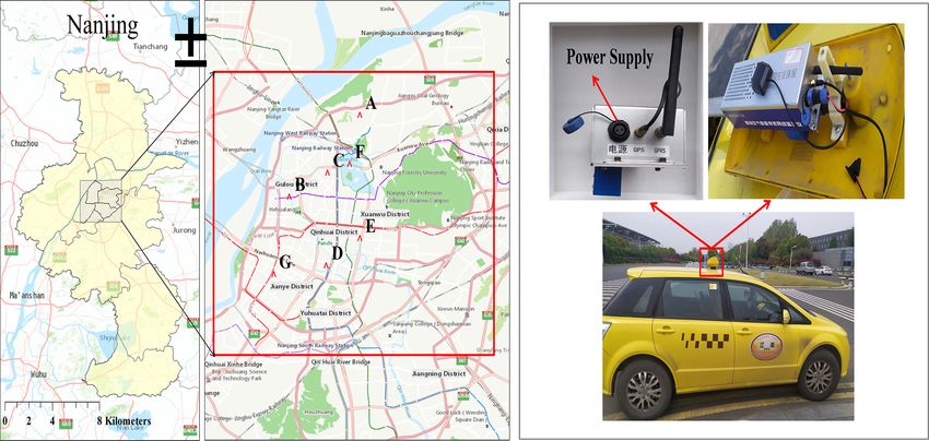
S. Wang et al.: Mobile monitoring of urban air quality                                                                                     7201

Figure 1. Location of the monitoring areas in the city of Nanjing (left) and photo of instrument installment (right). Red stars are the locations
of stationary stations belonging to the national air quality measurement network of China. These stations cover different functional regions
of the city: A, B, C, D, E, F, and G represent industrial, cultural and educational, commercial, traffic, residential, ecological park, and new
urban areas, respectively. Map credit: ESRI 2020.

sensitivity, so it is important that calibration procedures are            is that the air pollutant concentrations observed at SORPES
applied with respect to these limitations (Maag et al., 2018;              are lower than those observed in a road environment, which
Lösch et al., 2008). For example, environmental conditions                 might cause issues for the calibration process. Comparing
are known to cause nonlinear behavior of sensors (Popoola                  different calibration models, we found that a machine learn-
et al., 2016). Due to aging and impurity effects over a long               ing algorithm can improve sensor–monitor agreement with
time, low-cost sensors are prone to signal drift and low sensi-            reference monitors, and many previous studies have used this
tivity (Kizel et al., 2018). In addition, cross-sensitivities dif-         method (Qin et al., 2020; Esposito et al., 2018; Vito et al.,
fer largely according to the ambient temperature and level of              2018). A supervised machine learning methodology based
gas the sensor is being exposed to (Lösch et al., 2008). So,               on the gradient boost decision tree (GBDT) is used for data
multi-parameter joint calibration training is utilized to reduce           calibration (Johnson et al., 2018). GBRT, an ensemble learn-
the interference issue between air pollutants in our research,             ing method, is a decision-tree-based regression model that
including air pollutant concentrations, temperature, and rela-             implements boosting to improve model performance using
tive humidity. The sensors are usually trained with co-located             both parameter selection and k-fold cross-validation. GBRT
data collected by reference methods before being deployed                  needs to be trained by the dataset with target labels (Yang
to actual measuring campaigns (Kaivonen and Ngai, 2020;                    et al., 2017). It takes input variables including raw signals
Chatzidiakou et al., 2019; Bossche et al., 2015).                          of sensors, air pollutant concentrations (CO, NO2 , and O3 ),
   The XHAQSN-508 is calibrated every month starting from                  temperature, and relative humidity. The stationary instrument
September 2019. The instrument is placed at the outdoor                    data are taken as training targets. The parameters of the ma-
Station for Observing Regional Processes of the Earth Sys-                 chine learning model are adjusted continuously based on a
tem (SORPES) in the Xianlin Campus of Nanjing University                   gradient descent algorithm. The R 2 of the calibration results
(https://as.nju.edu.cn/as_en/obsplatform/list.htm, last access:            is generally high (> 0.90) for all the three air pollutants (e.g.,
22 May 2021) for at least seven days before the taxi be-                   Fig. 2a).
gan sampling. The collected data are calibrated against stan-                 The success of supervised model training with target la-
dard instruments (Thermo Fisher Scientific 48i, 42i, and 49i,              bels (i.e., co-located with SORPES, Fig. 2a) does not guar-
USA, for CO, NO2 , and O3 , respectively). The instrument                  antee its predicting power for conditions without labels
precision is ±2 ppbv for O3 and ±1 % and ±4 % for CO and                   (i.e., on roads or co-located with SORPES but not feed-
NO2 , respectively, which have been used in many other stud-               ing the station data to the algorithm; Fig. 2b). We use a
ies and found to perform well for long-term runs (Ding et                  calibration–validation methodology to evaluate the perfor-
al., 2013; Herrmann et al., 2013). One drawback of our study               mance of the calibrated sensors (Chatzidiakou et al., 2019).

https://doi.org/10.5194/acp-21-7199-2021                                                      Atmos. Chem. Phys., 21, 7199–7215, 2021
7202                                                                  S. Wang et al.: Mobile monitoring of urban air quality

This method includes two phases: first, the sampler was cali-       with 50 m × 50 m resolution and calculate the mean values
brated against the SORPES station for 10 d (1–10 June 2020),        of the samples collected in each grid. The driving condition
and the sensor data were used for sensor algorithm train-           is highly variable and the taxi can travel more than 50 m in
ing as described above (Fig. 2a); second, we continued to           10 s if the vehicle speed is over 18 km/h. However, given
place the sampler in the station (11–17 June 2020). How-            the complexity of the driving conditions, we ignore the vehi-
ever, the sensor data are not used for calibration but directly     cle trajectory in the past 10 s but assign the measured values
fed in the algorithm trained in the first phase. The results        to the location of the vehicle at the time of data uploading.
are compared with the station data (i.e., validation phase;         Then, combined with GIS technology, we calculate the aver-
Fig. 2b). We find that the sensor data agree well with standard     age of all the data points over one year that fall in the same
instrumentation in the second phase. The sensor-retrieved           grid. One drawback of our study is the impact of spike con-
CO, NO2 , and O3 concentrations are 0.58 ± 0.12 mg m−3 ,            centrations on sensor performance. The sensors keep report-
8.40 ± 4.30 µg m−3 , 27.3 ± 16.5 µg m−3 respectively, not sig-      ing high concentrations in an approximate 1 min period after
nificantly different from those measured by standard in-            exposure to large environmental concentration spikes. This
struments (0.50 ± 0.10 mg m−3 , 10.5 ± 6.31 µg m−3 , and            effect would reduce the effective resolution of our gridded
32.4 ± 20.2 µg m−3 ) (α = 0.05, ANOVA analysis). The R 2            concentration map. Similarly, we calculate the hourly aver-
values generally remain high (0.82–0.97) for different air          age concentrations by considering only the data sampled in
pollutants (CO and O3 ) except for NO2 (R 2 = 0.67). The            the same hour of different days. The GPS signal is missing
lower R 2 value for NO2 may be associated with the higher           when the taxis pass through the nine underground tunnels in
humidity during the validation period (13–16 June 2020). As         Nanjing (e.g., Xuanwu lake tunnel and Jiuhuashan tunnel in
NO2 is water dissolvable, high relative humidity may lead to        the city center; Fig. 3). We assume the taxies travel at a con-
a low bias for sensors (Wei et al., 2018). To improve perfor-       stant speed and the sampling points are uniformly allocated
mance of the NO2 model, temperature and relative humidity           along the tunnels. We use the ArcGIS 10.2 software for data
have also been involved in the training algorithm. However,         processing. To calculate the air pollutant concentrations (CO,
the interaction between O3 and NO2 may influence the de-            NO2 , and O3 ) of different road types and the contribution of
tection accuracy of these two chemicals, especially for NO2         traffic emissions to them, we divide the urban roads in Nan-
(Ivanovskaya et al., 2001). The accuracy of the sensor gen-         jing area into six types, including highways, arterial roads,
erally decreases with time (a.k.a. aging) due to the evapo-         secondary roads, branch roads, residential streets, and tun-
ration of the electrolyte (Ribet et al., 2018). However, we         nels (https://wiki.openstreetmap.org/wiki/Key:highway, last
find no significant decrease in the R 2 values for the three        access: 21 January 2021). The roads and land use data of
pollutants during our campaign. It seems that the machine-          Nanjing shown in Fig. 3 are based on OpenStreetMap (Open-
learning algorithm could successfully compensate the aging          StreetMap contributors, 2020).
of the sensors. Field calibration of low-cost sensors is still
a challenging task, as it is greatly affected by atmospheric        2.4   Traffic source attribution
composition and meteorological conditions (Spinelle et al.,
2017; Castell et al., 2017). Our results have high R 2 values       The mobile platform keeps sampling in the urban road net-
compared to previous studies, indicating relatively high ac-        work which carries a strong signal from traffic sources. By
curacy (e.g., Castell et al., 2017). The results from the two       contrast, stationary stations are often located far away from
sensors also agree with each other reasonably well, with R 2        major roads to represent a regional background air pollu-
values ranging 0.97–0.99 for a linear regression. Their data        tion level (Hilker et al., 2019). Seven state-operated air qual-
are thus combined in the following analysis to achieve max-         ity observation stations in Nanjing are selected in our re-
imum data coverage. Overall, the sensor results have sub-           search, including Maigaoqiao, Caochangmen, Shanxi Road,
stantial uncertainty compared to reference methods. We thus         Zhonghuamen, Ruijin Road, Xuanwu Lake, and the Olympic
focus on the relative temporal and spatial distributions rather     Sports Center (Zhao et al., 2015; Zou et al., 2017), which
than the absolute concentrations.                                   are far away from major roads and large point sources, so
                                                                    they are usually used as regional backgrounds in different
2.3    Data processing                                              functional areas (Zou et al., 2017; An et al., 2015). For ex-
                                                                    ample, Zou et al. (2017) chose the Olympic Center station
As the mobile monitoring platform samples along the tra-            (G in Fig. 1) to get the background characteristics of CO and
jectories of carrying vehicles, we need to sacrifice either the     NO2 in Nanjing. Therefore, the normalized contribution from
temporal information to calculate the spatial distribution of       traffic-related emissions can be obtained by differencing the
air pollutants, or the spatial information to temporal varia-       mobile measurements and the stationary ones to minimize
tions. Similar approaches have also been adopted by previous        the influence of daily meteorological variations on the urban
studies (Bossche et al., 2015; Apte et al., 2017; Farrell et al.,   air quality, following Bossche et al. (2015):
2015). To generate the spatial distribution of air pollutants at
high spatial resolution, we divide the research area into grids

Atmos. Chem. Phys., 21, 7199–7215, 2021                                               https://doi.org/10.5194/acp-21-7199-2021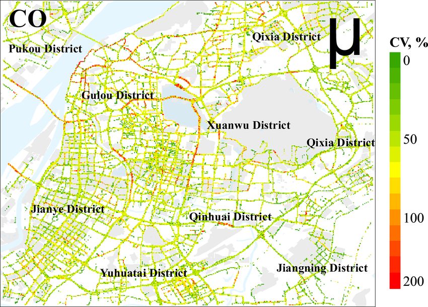
S. Wang et al.: Mobile monitoring of urban air quality                                                                       7203

Figure 2. Sensor performance evaluated by a calibration-validation methodology for CO, NO2 , and O3 . (a) Calibration period (1–
10 June 2020); (b) validation period (11–17 June 2020). The time series plots compare the concentrations measured by the co-located
sensors and standard instruments, while the scatterplots show pollutant concentrations and linear regressions between them.

                                                                    Fig. 1). We refer to this method as the “background site”
                                                                    (BS).
                                                                       We also adopt a method similar to Apte et al. (2017) for
                                                                    traffic source attribution. This method includes a peak de-
                                                                    tection algorithm to calculate the contribution of local traf-
                                                                    fic emission sources to on-road pollutant concentrations. We
                                                                    calculate the mean and minimum of air pollutant concentra-
                                                                    tions in each grid as the “peak” and “baseline”, respectively.
                                                                    The difference between the two is considered as the contri-
                                                                    bution from traffic sources. We refer to this method as “peak
                                                                    detection” (PD). MATLAB R2019a is used for such data cal-
                                                                    culation.

                                                                    3     Results and discussion

Figure 3. Locations of tunnels in Nanjing urban area. © Open-       3.1    Effect of spatial resolution on reproducibility
StreetMap contributors 2019. Distributed under a Creative Com-
mons BY-SA License.                                                 There is a trade-off between the resolution of an air pol-
                                                                    lutant concentration map and its reproducibility; i.e., high-
                                                                    resolution maps are subject to large randomness due to the
                                                                    limited number of samples in each grid. We investigate the
                                                                    consistency of spatial patterns of different resolution (10–
APtraffic,ij = (APij − APmin )/APij ,                       (1)     100 m). We calculated the standard error of the means of
                                                                    samples in each grid (SEM) and then averaged the SEM over
where APtraffic,ij represents the air pollutant concentration       all grid cells:
contributed by traffic emissions for the ith pollutant at time
                                                                            √
j (%); APij is the sensor-measured concentration of air pol-        SEM = σ/ n ,                                               (2)
lutants; and APmin means the ambient background concen-
tration, which is calculated as the minimum of the measure-         where σ and n are the standard deviation and number of sam-
ments from all the stations in Nanjing in the national air qual-    ples in each grid, respectively. We find the calculated SEM
ity network without major sources within a direct vicinity of       first decays rapidly with the grid spacing but tends to be in
50 m (https://quotsoft.net/air/, last access: 1 November 2020,      a regime of linear decay after a resolution of approximately

https://doi.org/10.5194/acp-21-7199-2021                                             Atmos. Chem. Phys., 21, 7199–7215, 2021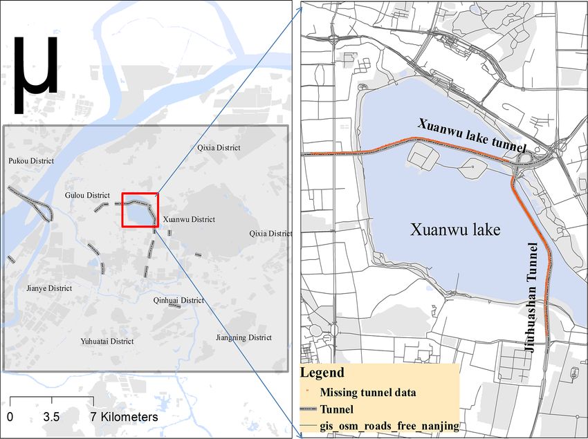
7204                                                                  S. Wang et al.: Mobile monitoring of urban air quality

                                                                    ally higher than previous research on mobile monitoring of
                                                                    urban air pollution (Peters et al., 2013; Poppel et al., 2013;
                                                                    Bossche et al., 2015; Apte at al., 2017), which can lower the
                                                                    uncertainty of our results. By comparing the time series of
                                                                    the air pollutant concentrations with that from nearby state-
                                                                    operated air quality observation stations (A0 and E0 , with re-
                                                                    peated frequencies > 500), we find that the results are con-
                                                                    sistent (Fig. S1 in the Supplement), which shows the stability
                                                                    and reliability of our data.

                                                                    3.3   Variability analysis

                                                                    Figures 6 and S2 show the coefficients of variation (CV ≡
                                                                    standard deviation / mean × 100 %) for different air pollu-
                                                                    tants in each grid. For one thing, this matrix quantifies the
                                                                    sensing power of mobile monitoring, i.e., more data points
                                                                    reduce the uncertainty of observations. For another, it reflects
Figure 4. Relationship between grid resolution and the domain-      the inherent variability of pollutants caused by factors such
averaged standard error of the mean of samples in each grid (SEM)   as meteorological conditions and hotspot emission sources.
for CO, NO2 , and O3 .
                                                                    We find that the CV values are lower than 100 % on the main
                                                                    roads, including highways and arterial roads, but higher than
                                                                    100 % on some tunnels, residential streets, and Nanjing rail-
50 m for all the three air pollutants (Fig. 4). Therefore, we       way station. As discussed above, the road network coverage
choose a resolution of 50 m, which is consistent with pre-          is much higher over the main roads than smaller roads. This
vious studies (Bossche et al., 2015; Apte et al., 2017). For        indicates that increasing the sampling numbers within sec-
example, Bossche et al. (2015) used a spatial resolution of         ondary and residential roads is the most useful way to reduce
20–50 m to map urban air quality and identify hotspots. Apte        the uncertainty of mobile observation. It is also interesting to
et al. (2017) found that reproducible results (with high pre-       note that a single taxi has a data coverage of ∼ 37 % but the
cision and low bias) of NO, NO2 , and black carbon can be           second one only increases it by ∼ 6.5 % to 43.5 %, which im-
generated by at least 10–25 repetitions in a specific area with     plies that the marginal increase in spatial coverage decreases
30 m median spatial aggregation.                                    substantially with an increasing number of sensors. This is
                                                                    indeed one limitation of our monitoring platform, and a much
3.2    Road network coverage                                        larger fleet size or different sampling platforms (e.g., bikes)
                                                                    may be needed to reduce the uncertainty over these smaller
A total of 1.32 million pieces of data were obtained dur-           roads.
ing the observation period, which covers 66.4 % of the ma-             Although the spatial patterns of CV are similar for dif-
jor roads in Nanjing in the sampling domain with a large            ferent air pollutants, we find generally higher CV for O3
repeat-visit frequency (median repetition = 61 (14 and 264          (67.3 %) and NO2 (59.5 %) than CO (51.6 %). This is as-
as the lower and upper quartiles, respectively, the same here-      sociated with the spatial and temporal variability of differ-
inafter)) (Fig. 5a). The type of road with the most visits is       ent air pollutants, which are influenced by their lifetimes in
the Neihuan lines (258 (116, 526)), followed by the arterial        the atmosphere. Lifetime (or residence time) is the average
roads (125 (35, 393)), secondary roads (151 (24, 442)), and         time for a chemical compound that is transported in the at-
highways (34 (12, 115)). The residential streets (22 (6, 100))      mosphere before it is deposited or consumed by chemical
have the fewest visits.                                             reactions. It is associated with its spatial scale of variabil-
   Apart from the areas without roads, such as the Yangtze          ity. The longer the lifetime, the more uniformly the concen-
River, Xuanwu Lake, and Purple Mountain, the data cover             trations are distributed. The chemical properties of CO are
43.5 % of the 50 m grids in the research area with the two          the most stable in the environment (τ = 1–2 months), and its
taxis contributing 36.8 % and 37.2 %. As shown in Fig. 5b,          spatial concentration difference is more affected by the sam-
the median number of repeated frequency in each grid is 66          pling time and the number of samples. The lifetime of NOx
(18, 286), with the highest value of 15 449 in Nanjing South        is shorter (τ = 2–11 h, Romer et al., 2016), so the measured
Railway Station and the lowest in some residential roads (1).       concentrations are more influenced by local or “hotspot”
The repeated frequencies in each 50 m grid along the arte-          emissions and meteorological factors. O3 has the shortest
rial roads and Neihuan line are higher than other types of          lifetime (τ =∼ 1 h in urban atmosphere, McClurkin et al.,
roads, i.e., Zhongyang road, Huju road, Neihuandong, and            2013) among the three pollutants. The level of ozone is af-
Neihuanxi lines (Fig. 5b). Our repeated frequency is gener-         fected by its precursors (NOx and VOCs), which both have

Atmos. Chem. Phys., 21, 7199–7215, 2021                                               https://doi.org/10.5194/acp-21-7199-2021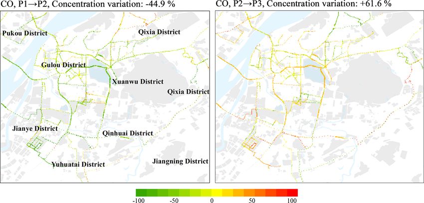
S. Wang et al.: Mobile monitoring of urban air quality                                                                         7205

Figure 5. Mobile monitoring data coverage with regard to roads (a) and 50 m grids (b). © OpenStreetMap contributors 2019. Distributed
under a Creative Commons BY-SA License.

                                                                     stations. A total of 17 hotspots for CO and NO2 , and 17
                                                                     hotspots for O3 are identified, and the specific information
                                                                     is shown in Fig. 7 and Table 1. Most of the “hotspots” show
                                                                     relatively apparent spatial “peaks” for multiple pollutants.
                                                                     To identify the main sources contributing to these hotspots,
                                                                     we use the different relative concentrations of the measured
                                                                     pollutants (Zhao et al., 2015). We also use field informa-
                                                                     tion around hotspot areas, such as the existence of subway
                                                                     stations, construction sites, factories, and restaurants nearby.
                                                                     This method has substantial uncertainties in terms of the at-
                                                                     tribution of the potential sources to these “hotspots”, and
                                                                     further source–receptor relationships and detailed chemical
                                                                     component analyses are required to identify the exact emis-
                                                                     sion sources.
                                                                        We find that “hotspots” are mainly affected by one of
                                                                     the three types of emission sources, namely traffic emis-
Figure 6. Spatial distribution of coefficient of variation for CO
in 50 m grids in research domain. © OpenStreetMap contributors       sions (diesel and gasoline on-road vehicle exhaust), indus-
2019. Distributed under a Creative Commons BY-SA License.            trial emissions, and cooking fumes. The mean CO and
                                                                     NO2 concentrations are relatively high at the crossroads (E,
                                                                     1.47 mg m−3 and 15.8 µg m−3 ), tunnels (B, 1.24 mg m−3 and
large variability (Sharma et al., 2016). The complex chemical        16.6 µg m−3 , respectively), the roads near the hospital (H,
reactions also increase its spatial heterogeneity.                   0.66 mg m−3 and 15.7 µg m−3 ), and near the railway sta-
                                                                     tion (A, 0.60 mg m−3 and 4.0 µg m−3 ), which are affected
3.4     Spatial distribution                                         by on-road traffic emissions. In addition, due to the con-
                                                                     struction of Maigaoqiao subway station (G, 0.91 mg m−3 and
3.4.1    Hotspot identification                                      11.8 µg m−3 ), diesel vehicles and off-road traffic emission
                                                                     also make a great contribution to CO and NO2 concentra-
Although the instantaneous pollution level varies drastically        tions. Industrial emissions from petrochemical enterprises (I)
in different road environments, we obtain a relatively robust        also lead to high NO2 concentrations (0.26–93.1 µg m−3 ) on
time-integrated pollution estimate by calculating the mean           surrounding roads.
of repeated samples (Fig. 7). We define the area where the              As shown in Fig. 7, the higher O3 concentrations in these
pollutant concentrations are 50 % higher than nearby grids           hotspot areas are mainly caused by higher NOx and VOC
(radius = 300 m) as “hotspots” following Apte et al. (2017).         emissions from the heavy traffic (W, 46.8 ± 27.4 µg m−3 ;
The pollutant concentrations shown in Table 1 are the val-           Xie et al., 2016; Ding et al., 2013), cooking emissions
ues after deducting the background concentration, which are          (Q, 38.5 ± 26.0 µg m−3 ), and ozone precursors from in-
calculated by the annual mean concentration of stationary            dustrial emissions (e.g., K, 47.1 ± 36.5 µg m−3 , and J,

https://doi.org/10.5194/acp-21-7199-2021                                              Atmos. Chem. Phys., 21, 7199–7215, 2021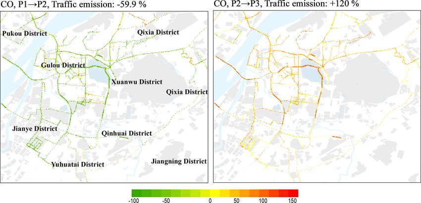
7206                                                                  S. Wang et al.: Mobile monitoring of urban air quality

37.6 ± 25.8 µg m−3 ), such as VOCs. In addition, bio-
genic VOC emissions also have a significant impact on
the formation of ozone (U, 40.4 ± 18.3 µg m−3 , and V,
33.5 ± 20.4 µg m−3 ; Liu et al., 2018). Taxi sensor data also
reveal the secondary pollution characteristics at the micro-
scale, showing that O3 concentration in the downtown area
with dense buildings is significantly higher than that in other
areas, especially some residential areas in Jianye and Gulou
district. Previous studies have also found that the air pollutant
“hotspots” are associated with traffic-related emissions (e.g.,
heavy-duty diesel vehicles, Targino et al., 2016, and vehicle
congestion, Gately et al., 2017) and high-density urban areas
(Li et al., 2018). These identified air pollution “hotspots”,
and the diagnosed source contributions provide helpful in-
formation for urban air quality management, which demon-
strates the sensing power of mobile monitoring deployed on
a taxi fleet.

3.4.2   Air pollutant concentrations in different types of
        roads

We find that air pollutant levels differ vastly among the
six types of roads (p < 0.05, with the ANOVA method).
The mean CO and NO2 concentrations follow this trend:
tunnels (2.22 ± 1.18 mg m−3 and 40.7 ± 29.7 µg m−3 ,
respectively) > highways (1.10 ± 0.59 mg m−3 and
29.2 ± 8.66 µg m−3 ) > arterial roads (0.958 ± 0.308 mg m−3
and        25.0 ± 6.90 µg m−3 )    >     secondary     roads
(0.855 ± 0.401 mg m−3 and 21.8 ± 8.89 µg m−3 ) > branch
roads (0.818 ± 0.216 mg m−3 and 20.3 ± 6.79 µg m−3 )
> residential streets (0.783 ± 0.299 mg m−3               and
19.7 ± 8.35 µg m−3 ) (Table 2). However, the mean
O3 concentrations in different types of roads are
opposite to that of CO and NO2 : residential streets
(35.1 ± 15.4 µg m−3 ) > branch roads (32.7 ± 12.2 µg m−3 )
> secondary roads (31.9 ± 10.0 µg m−3 ) > arterial roads
(29.6 ± 7.52 µg m−3 ) > highways (23.3 ± 9.12 µg m−3 ) >
tunnels (15.7 ± 7.85 µg m−3 ).
   The differences of air pollutant concentrations among dif-
ferent road types are firstly affected by the traffic-related
emission sources including vehicle engine exhaust, which is
a function of traffic flow and speed, vehicle type, etc. (Sa-
hanavin et al., 2018). The general decreasing trends we ob-
served for CO and NO2 are consistent with traffic flow and
the congestion index in the Nanjing urban area (Table 2, Zou
et al., 2017). Apte et al. (2017) also found that the NO2
concentration decreased in turn on highways, arterial roads,
and residential streets, which are in good agreement with           Figure 7. Spatial distribution and “hotspots” of air pollutant con-
our research. The observed O3 concentrations have oppo-             centrations in the research domain (CO, NO2 , and O3 ). Circles
site trends of CO and NO2 with the highest concentration            marked with A–Z represent the identified “hotspots”, where the air
in residential streets (Table 2). As O3 production in Nan-          pollutant concentrations are at least 50 % higher than the surround-
jing is in VOC-limited regions, lower NOx could reduce              ing area (300 m radius). © OpenStreetMap contributors 2019. Dis-
its titration of O3 and subsequently increase O3 concentra-         tributed under a Creative Commons BY-SA License.
tion (Ding et al., 2013; Xie et al., 2016). The O3 concen-
trations are lowest in tunnels, which is associated with the

Atmos. Chem. Phys., 21, 7199–7215, 2021                                                https://doi.org/10.5194/acp-21-7199-2021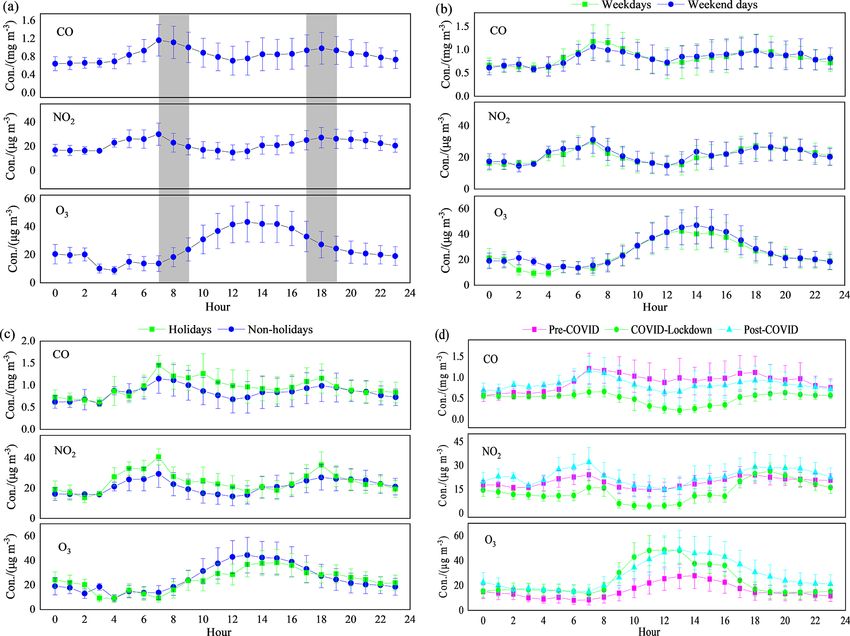
S. Wang et al.: Mobile monitoring of urban air quality                                                                                  7207

Table 1. “Hotspots” of air pollution for multi-pollutants identified in Nanjing. “No.” refers to the number of observation points within 300 m
of the hotspots.

            ID    Specific        No.    CO, mg m−3       NO2 , µg m−3     Description/potential sources
            A     A1, A2         6535      0.60 ± 0.82       4.0 ± 15.9    Nanjing railway station/gasoline vehicle emission
            B     B1, B2, B3     4177      1.24 ± 1.74      16.6 ± 26.1    Exit and entrance of tunnel/gasoline vehicle emission
            C     C              1002      0.73 ± 0.39      0.90 ± 12.5    Subway entrance/gasoline vehicle emission
            D     D1–D5          4333      0.46 ± 0.61      6.10 ± 15.0    Overpass on ring road/vehicle emission
            E     E1, E2         5354      1.47 ± 3.04      15.8 ± 26.8    Crossroads/vehicle emission
            F     F              1052      0.55 ± 0.53      13.5 ± 14.2    Moonlight Plaza/vehicle emission
            G     G              6160      0.91 ± 1.31      11.8 ± 21.0    Maigaoqiao subway station/diesel vehicle emission
            H     H              6231      0.66 ± 0.74      15.7 ± 23.5    Hospital/vehicle emission
            I     I              2386      0.36 ± 0.49      5.60 ± 14.0    Petrochemical enterprises/industrial emissions

weak sunlight in the tunnels (Awang et al., 2015). Further-               al. (2004) observed a significant weekend effect in southern
more, due to the unfavorable diffusion conditions in the tun-             California, showing that during the morning traffic rush hour,
nels, NO2 concentration is accumulated to a relatively high               the concentrations of CO and NO2 at weekends were about
level (40.7 ± 29.7 µg m−3 ), which titrates O3 . The tunnel also          18 % and 37 % lower than on weekdays. The difference be-
blocks the replenishment of surrounding O3 -rich air, result-             tween our study and other cities lies in the difference of fleet
ing in a lower O3 concentration than other roads (Kirchstetter            fuel structure, and the different weekly routine of human ac-
et al., 1996).                                                            tivities and the taxi driving trajectories (Xie et al., 2016).
                                                                             The median concentrations of CO and NO2 during hol-
3.5   Temporal variation                                                  idays are comparable to those during non-holidays but are
                                                                          18.3 % lower for O3 (Fig. 8c). In addition, compared with
Figure 8 shows the temporal variation of the three air pol-               the spatial distribution of O3 concentration during holi-
lutant concentrations during the observation campaign, with               days, we find that the concentrations of O3 in Xinjiekou
the hourly mean concentrations over the research domain                   and its surrounding areas, where many shopping malls are
shown in Fig. 9 (the corresponding spatial distributions are              located, are higher during non-holidays (Fig. S6). This
shown in Figs. S4–6). The difference of the hourly varia-                 may be related to the higher NO2 concentrations in this
tion of the mean sample of different types of roads over a                area during holidays (24.8 ± 10.2 µg m−3 ) than non-holidays
year is small (Fig. S7), so the data in Fig. 9 are not filtered           (20.6 ± 4.82 µg m−3 ). The hourly concentrations show no
in anyway, but for each hour a similar mix of road types                  significant difference between holidays and non-holidays
is sampled. We find that the median concentrations of CO                  (Fig. 9c). The holidays include the periods of National Day
and NO2 in rush hours (07:00–09:00 and 17:00–19:00 LT)                    (1–7 October), the Spring Festival (24–31 February), Qing-
are increased by 26.4 % and 27.3 % compared to non-rush                   ming Festival (4–6 April), international labor day (1–5 May),
hours, respectively. The hourly mean concentrations of CO                 and the Dragon Boat Festival (25–27 June). The “holiday ef-
and NO2 show a double-peak pattern with higher concen-                    fect” has been observed extensively for urban and regional air
trations in rush hours (Fig. 9a), reflecting the contribution             quality. For example, Xu et al. (2017) found that VOC tracers
of traffic-related emissions (Tan et al., 2009), which we will            were significantly enhanced during the National Day holiday
elaborate in the next section. The observed O3 concentrations             (from 1–10 October 2014) in the Yangtze River Delta (YRD)
show a unimodal diurnal pattern with a peak at ∼ 14:00 LT                 region, indicating that the “holiday effect” had a strong influ-
as a result of photochemical formation. At night, O3 concen-              ence on the distribution and chemical reactivity of VOCs in
trations are maintained at a low level due to a lack of solar             the atmosphere. The reason why this effect is not observed
radiation and the NOx -titration effect (Xie et al., 2016; Li et          in our study may be related to the relatively smaller sample
al., 2013). These patterns generally agree with the measure-              size during holidays. The sample size for holidays account
ments at stationary monitoring stations (Fig. S3).                        for only 11.3 % of those for the non-holidays.
   No significant differences are observed for the median
concentrations and spatial distribution of three air pollutants           3.6   Traffic source contribution
between weekdays and weekends (α = 0.05; Figs. 8b and
S4), even though the morning peaks for CO are slightly                    Figure 10a and b show the calculated contributions by
higher during weekdays (Fig. 9b), which is consistent with                traffic-related emission sources to the observed concentra-
An et al. (2015). Wang et al. (2014) found that NOx displays              tion of CO (referred to as contributions hereinafter). We
a weekly cycle in the Beijing–Tianjin–Hebei metropolitan                  find that the mean contribution calculated by the BS method
area, with higher levels on weekdays than weekends. Qin et                (42.6 ± 11.5 %) is generally consistent with that obtained

https://doi.org/10.5194/acp-21-7199-2021                                                    Atmos. Chem. Phys., 21, 7199–7215, 2021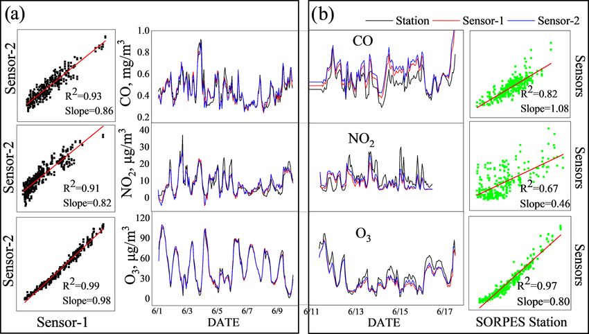
7208 S. Wang et al.: Mobile monitoring of urban air quality
Table 2. Multi-pollutant concentrations for six types of roads.
Road types Road numbers Vehicle speed, Traffic congestion CO, NO2 , O3 ,
km/h index∗ mg m−3 µg m−3 µg m−3
Tunnels 9 – – 2.22 ± 1.18 40.7 ± 29.7 15.7 ± 7.85
Highways 168 60–80 2.18 1.10 ± 0.594 29.2 ± 8.66 23.3 ± 9.12
Arterial 443 40–60 1.78 0.958 ± 0.309 25.0 ± 6.90 29.7 ± 7.53
Secondary 419 30–50 1.70 0.855 ± 0.401 21.8 ± 8.89 31.9 ± 10.0
Branch roads 349 20–40 – 0.818 ± 0.216 20.3 ± 6.79 32.7 ± 12.2
Residential 152 < 20 – 0.783 ± 0.230 19.6 ± 8.35 35.1 ± 15.5
∗ The traffic congestion index data are from the Gaud map https://report.amap.com/detail.do?city=320100 (last access: 24 October 2020).
Figure 8. Variation of pollutants concentrations in rush/non-rush hours, weekdays/weekend days, holidays/non-holidays, and three stages of
the COVID-19 pandemic. The dot in each box represents the mean value and the solid line represents the median value. Each box extends
from the 25th to the 75th percentile. The whiskers (error bars) below and above the boxes represents the 10th and 90th percentiles.
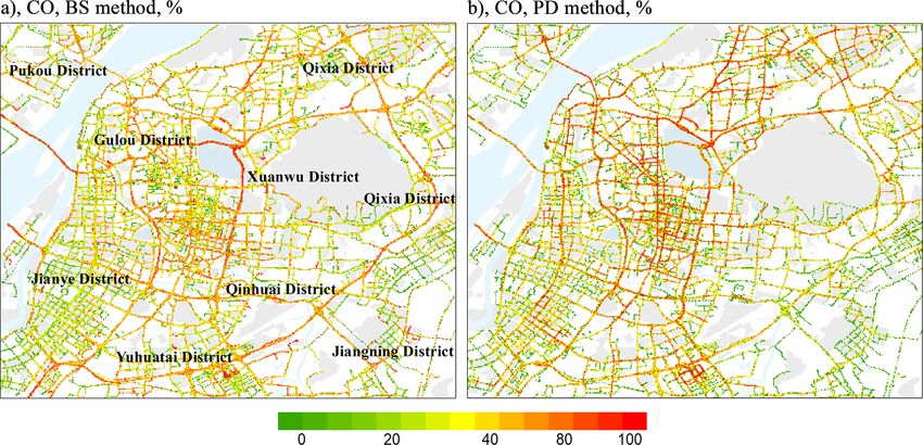
from the PD algorithm (43.9 ± 27.0 %). Their spatial patterns sistent with the trend in traffic volumes. The patterns for NO2
are also similar (Fig. 10a vs. b). Although our data coverage are quite similar to CO (Fig. S8c and d, Table 1), but the
is much larger than that of the Apte et al. (2017) study, we mean contribution to NO2 calculated using the BS method
find that the reference method is still applicable in our re- (26.3 ± 14.7 %) is lower than that obtained from the PD al-
search area. The contributions in highways, near tunnel en- gorithm (40.2 ± 29.9 %). This difference is associated with
trances and exits (e.g., Jiuhuashan and Xuanwuhu tunnel), the relatively higher uncertainty for NO2 measurements by
at the railway station (Nanjing south station), and on arte- sensors (Sect. 2.2), while the results of the PD method seem
rial roads (44 %–59 %) calculated using both methods are unaffected as the sensor bias is canceled out when calculating
higher than on secondary roads and residential streets and the difference between “peak” and “baseline” (Sect. 2.4).
lowest on branch roads (29 %–39 %) (Table 3), which is con-
Atmos. Chem. Phys., 21, 7199–7215, 2021 https://doi.org/10.5194/acp-21-7199-2021S. Wang et al.: Mobile monitoring of urban air quality 7209
Figure 9. Diurnal cycles of three pollutants concentrations measured in rush/non-rush hours, weekdays/weekend days, holidays/non-
holidays, and different stage of the COVID-19 pandemic by the taxi sensors. Error bars in panel a show the standard deviation of observations.
Gray areas represent the rush hours, and the other represents the non-rush hours (a).
The bottom-up emission inventory indicates that on-road butions are also depicted in Figs. 11–12 and S9–S10. We
transportation contributed ∼ 11 % of total CO emissions divide the data into three stages: pre-COVID (P1, 1 Oc-
from Nanjing in 2012 (Zhao et al., 2015). Considering the tober 2019–23 January 2020), COVID lockdown (P2, 24–
number of cars has increased by ∼ 80 % and the total CO 31 January 2020 and 17–24 February 2020), and post-
emissions remained relatively stable (BSNM, 2019), the con- COVID (P3, 1 March–30 September 2020). We find the me-
tribution of traffic sources in recent years is expected to be dian concentrations of CO and NO2 were the lowest in P2
∼ 20 %. These values are much lower than what we cal- (Fig. 9d). For example, the CO and NO2 concentrations de-
culated based on mobile monitoring data because of the creased by 44.9 % and 41.7 % from P1 to P2, respectively
lower spatial resolution of these regional inventories (e.g., (Figs. 11 and S8). This pattern agrees well with the air quality
0.05◦ × 0.05◦ ) (Zheng et al., 2014). They are unable to dis- station data over eastern China (Huang et al., 2021). We fo-
tinguish the emission characteristics of air pollutant within cus on the traffic sector as it is the most sensitive to lockdown
a street level (tens of meters), which leads to their under- measures, while other sectors, including power, industrial,
estimation of traffic-related emissions in the road micro- and residential sectors, remain relatively unchanged (Gue-
environment. vara et al., 2021). We find that from P1 to P2, the average traf-
fic source contributions of CO and NO2 using the BS method
3.7 Impact of COVID-19 pandemic decreased by 59.9 % and 51.8 %, respectively (Figs. 12 and
S9). This is consistent with the transportation index data,
Figures 8d and 9d show the variation of air pollutant con- which shows a 70 % reduction in eastern Chinese cities dur-
centrations at different stages of the COVID-19 pandemic. ing lockdown (Huang et al., 2021).
The spatial distribution of concentrations and traffic contri-
https://doi.org/10.5194/acp-21-7199-2021 Atmos. Chem. Phys., 21, 7199–7215, 20217210 S. Wang et al.: Mobile monitoring of urban air quality
Figure 10. Contributions from traffic-related emissions calculated using the stationary data method (a) and peak detection algorithm (b) for
CO. © OpenStreetMap contributors 2019. Distributed under a Creative Commons BY-SA License.
Table 3. Contribution of traffic emissions to CO and NO2 in different roads using the two methods.
Road types Traffic emissions – CO, % Traffic emissions – NO2 , %
BS PD BS PD
Highways 48.3 ± 10.4 51.0 ± 20.4 32.5 ± 14.5 41.4 ± 22.5
Arterial 44.1 ± 9.23 59.0 ± 19.4 26.8 ± 10.6 43.6 ± 23.3
Secondary 40.2 ± 11.7 47.6 ± 23.9 22.8 ± 13.2 35.2 ± 25.1
Residential 39.4 ± 14.1 38.9 ± 26.1 20.3 ± 16.3 28.6 ± 25.0
Branch roads 39.2 ± 12.2 29.7 ± 23.9 21.5 ± 18.1 25.5 ± 24.4
The observed CO and NO2 concentrations recovered to a and solar insolation in P2 and P3 also favor the photochem-
level similar to P1 during P3. The traffic-related source con- ical formation of O3 compared to P1 (Xie et al., 2016; Fu et
tributions were increased by 120 % and 131 % from P2 to P3 al., 2015; Reddy et al., 2010).
for CO and NO2 (Figs. 11 and S9). Due to the limited data
size and spatial coverage (only on some arterial roads and
highways) during P2, the calculated contribution of traffic 4 Conclusions
emissions to air pollutants may be not directly comparable
to those shown in Fig. 9. But the changes in the contribu- Accurate assessment of human exposure to urban air pol-
tion match well with the changes in traffic volume and hu- lution requires a detailed understanding of the spatial and
man activities (Bao and Zhang, 2020). Our results also agree temporal patterns of air pollutant concentrations. Combin-
with top-down emission estimates from remote sensing data ing mobile monitoring with GIS technology, we obtained
(Zhang et al., 2020), which showed the total NO2 emissions high-resolution (50 m × 50 m) spatial distribution maps of
decreased by 31 %–44 % from P1 to P2 but increased 67 %– three air pollutants in the main urban area of Nanjing, which
85 % from P2 to P3. demonstrates well the spatial heterogeneity of pollutants at
The observed ozone concentrations show a different trend the micro-scales. We find that higher spatial resolution is use-
from other pollutants in the three stages. We find a pattern ful to identify hotspots that are mainly affected by three types
of P1 < P2 < P3 for O3 median concentrations (Fig. 8d). The of air pollution emissions sources, namely, traffic, industrial,
ozone concentration increased by 35.7 % from P1 to P2, and and cooking fumes. It also provides hints for air quality man-
48.7 % from P2 to P3 (Fig. S9). While the contribution of agement and emission source control.
traffic emissions to ozone first decreased by 32.5 % from P1 We calculate the contribution of traffic-related emissions
to P2 and then increased by 39.3 % in P2 to P3 (Fig. S10). to air pollutants in different grid points by combining mobile
This is firstly associated with less titration of NOx during P2 observation and station observation data. Compared with the
as discussed earlier. In addition, the increased temperature peak detection method, the station data method is more rea-
sonable for secondary pollutants such as O3 , while the former
Atmos. Chem. Phys., 21, 7199–7215, 2021 https://doi.org/10.5194/acp-21-7199-2021S. Wang et al.: Mobile monitoring of urban air quality 7211
Figure 11. Changes in observed CO concentration in the three stages of the COVID-19 pandemic. P1, P2, and P3 are for pre-COVID,
COVID-lockdown, and post-COVID periods, respectively. © OpenStreetMap contributors 2019. Distributed under a Creative Commons
BY-SA License.
Figure 12. Changes in the contributions of traffic-related sources to CO in the three stages of the COVID-19 pandemic calculated using the BS
method. P1, P2, and P3 are for pre-COVID, COVID-lockdown, and post-COVID periods, respectively. © OpenStreetMap contributors 2019.
Distributed under a Creative Commons BY-SA License.
is less affected by sensor bias. There are also some differ- Data availability. All validation data and data processing by GIS
ences in the contribution of traffic emissions to air pollutants used in this work can be accessed by contacting the authors.
in different types of roads. Due to the impact of the COVID-
19 pandemic, the mean concentrations of CO and NO2 de-
creased by 44.9 % and 47.1 %, respectively, during the lock- Supplement. The supplement related to this article is available on-
down in Nanjing, and the contribution of traffic-related emis- line at: https://doi.org/10.5194/acp-21-7199-2021-supplement.
sions also decreased by 59.9 % and 52.6 %. In contrast, the
concentration of O3 increased by 35.7 %, respectively. After
reopening, CO and NO2 concentrations rebounded by 61.6 % Author contributions. YZ designed the research. SW performed the
research. SW, YZ, ZW, and MY analyzed data. LW, XC, and AD
and 48.2 %, and the contribution of traffic emissions both in-
provided validation data. MY, YL, and QL helped with the data
creased by over 100 %, indicating the great impact of traffic analysis. MW, LZ, and YX provided the monitoring instrument. SW
emissions on urban air pollution. and YZ wrote the paper.
https://doi.org/10.5194/acp-21-7199-2021 Atmos. Chem. Phys., 21, 7199–7215, 20217212 S. Wang et al.: Mobile monitoring of urban air quality
Competing interests. The authors declare that they have no conflict and Hoek, G.: Contrast in air pollution components between
of interest. major streets and background locations: Particulate matter
mass, black carbon, elemental composition, nitrogen oxide
and ultrafine particle number, Atmos. Environ., 45, 650–658,
Special issue statement. This article is part of the special issue “Air https://doi.org/10.1016/j.atmosenv.2010.10.033, 2010.
Quality Research at Street-Level (ACP/GMD inter-journal SI)”. It Borrego, C., Coutinho, M., Costa, A. M., Ginja, J., Ribeiro,
is not associated with a conference. C., Monteiro, A., Ribeiro, I., Valente, J., Amorim, J.
H., Martins, H., Lopes, D., and Miranda, A. I.: Chal-
lenges for a new air quality directive: the role of moni-
Acknowledgements. We are grateful to the Station for Observing toring and modelling techniques, Urban Clim., 14, 328–341,
Regional Processes of the Earth System (SORPES) in Xianlin Cam- https://doi.org/10.1016/j.uclim.2014.06.007, 2015.
pus of Nanjing University for providing the background data for Bossche, J. V. D., Peters, J., Verwaeren, J., Botteldooren, D., Theu-
sensor calibration. The authors thank Rong Ye and Liang Luo for nis, J., and Baets, B. D.: Mobile monitoring for mapping spatial
sample collection. variation in urban air quality: Development and validation of a
methodology based on an extensive dataset, Atmos. Environ.,
105, 148–161, https://doi.org/10.1016/j.atmosenv.2015.01.017,
2015.
Financial support. This study was supported by the National
Bureau Statistics of Nanjing Municipal: Nangjing Statistical Year-
Key Research & Development Program of China (grant nos.
book, available at: http://tjj.nanjing.gov.cn/bmfw/njsj/ (last ac-
2016YFC0202000 and 2019YFA0606803), Jiangsu Innovative and
cess: 8 November 2020), 2019.
Entrepreneurial Talents Plan, and the Collaborative Innovation Cen-
Castell, N., Dauge, F. R., Schneider, P., Vogt, M., Lerner, U.,
ter of Climate Change, Jiangsu Province.
Fishbain, B., Broday, D., and Bartonova, A.: Can commer-
cial low-cost sensor platforms contribute to air quality mon-
itoring and exposure estimates?, Environ. Int., 99, 293–302,
Review statement. This paper was edited by Joel Thornton and re- https://doi.org/10.1016/j.envint.2016.12.007, 2017.
viewed by three anonymous referees. Cavellin, L. D., Weichenthal, S., Tack, R., Ragettli, M. S., Smar-
giassi, A., and Hatzopoulou, M.: Investigating the use of portable
air pollution sensors to capture the spatial variability of traffic-
related air pollution, Environ. Sci. Technol., 50, 313–320,
References https://doi.org/10.1021/acs.est.5b04235, 2016.
Chatzidiakou, L., Krause, A., Popoola, O. A. M., Di Antonio, A.,
An, J. L., Zou, J., Wang, J., Lin., X., and Zhu, B.: Differences Kellaway, M., Han, Y., Squires, F. A., Wang, T., Zhang, H.,
in ozone photochemical characteristics between the megac- Wang, Q., Fan, Y., Chen, S., Hu, M., Quint, J. K., Barratt, B.,
ity Nanjing and its suburban surroundings, Yangtze River Kelly, F. J., Zhu, T., and Jones, R. L.: Characterising low-cost
Delta, China, Environ. Sci. Pollut. Res., 22, 19607–19617, sensors in highly portable platforms to quantify personal expo-
https://doi.org/10.1007/s11356-015-5177-0, 2015. sure in diverse environments, Atmos. Meas. Tech., 12, 4643–
Apte, J. S., Kirchstetter, T. W., Reich, A. H., Deshpande, S. J., 4657, https://doi.org/10.5194/amt-12-4643-2019, 2019.
Kaushik, G., Chel, A., Marshall, J. D., and Nazaroff, W. W.: Con- Ding, A. J., Fu, C. B., Yang, X. Q., Sun, J. N., Zheng, L. F., Xie,
centrations of fine, ultrafine, and black carbon particles in auto- Y. N., Herrmann, E., Nie, W., Petäjä, T., Kerminen, V.-M., and
rickshaws in New Delhi, India, Atmos. Environ., 45, 4470–4480, Kulmala, M.: Ozone and fine particle in the western Yangtze
https://doi.org/10.1016/j.atmosenv.2011.05.028, 2011. River Delta: an overview of 1 yr data at the SORPES station, At-
Apte, J. S., Messier, K. P., Gani, S., Brauer, M., Kirchstet- mos. Chem. Phys., 13, 5813–5830, https://doi.org/10.5194/acp-
ter, T. W., Lunden, M. M., Marshall, J. D., Portier, C. J., 13-5813-2013, 2013.
Vermeulen, R. C. H., and Hamburg, S. P.: High-resolution Esposito, E., Vito, S. D., Salvato, M., Fattoruso, G., Bright, V.,
air pollution mapping with google street view cars: ex- Jones, R. L., and Popoola, O.: Stochastic Comparison of Ma-
ploiting big data, Environ. Sci. Technol., 51, 6999–7008, chine Learning Approaches to Calibration of Mobile Air Qual-
https://doi.org/10.1021/acs.est.7b00891, 2017. ity Monitors, in: Sensors, CNS 2016, Lecture Notes in Elec-
Awang, N. R., Ramli, N. A., Yahaya, A. S., and Elbayoumi, M.: trical Engineering, edited by: Andò, B., Baldini, F., Di Na-
High nighttime ground-level ozone concentrations in Kemaman: tale, C., Marrazza, G., Siciliano, P., vol 431, Springer, Cham,
NO and NO2 concentrations attributions, Aerosol Air Qual. https://doi.org/10.1007/978-3-319-55077-0_38, 2018.
Res., 15, 1357–1366, https://doi.org/10.4209/aaqr.2015.01.0031, Farrell, W. J., Cavellin, L. D., Weichenthal, S., Goldberg, M.,
2015. and Hatzopoulou, M.: Capturing the urban canyon effect on
Bao, R. and Zhang, A.: Does lockdown reduce air pollution? Ev- particle number concentrations across a large road network
idence from 44 cities in northern China, Sci. Total Environ., using spatial analysis tools, Build. Environ., 92, 328–334,
139052, https://doi.org/10.1016/j.scitotenv.2020.139052, 2020. https://doi.org/10.1016/j.buildenv.2015.05.004, 2015.
Bart, E., Jan P., Martine, V. P., Nico, B., and Arnout, S.: The Fu, T. M., Zheng, Y., Paulot, F., and Mao, J.: Positive but vari-
aeroflex: a bicycle for mobile air quality measurements, Sensors, able sensitivity of August surface ozone to large-scale warming
13, 221–240, https://doi.org/10.3390/s130100221, 2012. in the southeast United States, Nat. Clim. Change, 5, 454–458,
Boogaard, H., Kos, G. P. A., Weijers, E. P., Janssen, N. A. https://doi.org/10.1038/nclimate2567, 2015.
H., Fischer, P. H., Van der Zee, S. C., De Hartog, J. J.,
Atmos. Chem. Phys., 21, 7199–7215, 2021 https://doi.org/10.5194/acp-21-7199-2021You can also read