Worldwide lake level trends and responses to background climate variation - Articles
←
→
Page content transcription
If your browser does not render page correctly, please read the page content below
Hydrol. Earth Syst. Sci., 24, 2593–2608, 2020
https://doi.org/10.5194/hess-24-2593-2020
© Author(s) 2020. This work is distributed under
the Creative Commons Attribution 4.0 License.

Worldwide lake level trends and responses to background
climate variation
Benjamin M. Kraemer1,3 , Anton Seimon2 , Rita Adrian1 , and Peter B. McIntyre3,4
1 Ecosystem  Research Department, IGB Leibniz Institute of Freshwater Ecology and Inland Fisheries, Berlin, Germany
2 Department  of Geography and Planning, Appalachian State University, Boone, NC, USA
3 Center for Limnology, University of Wisconsin–Madison, Madison, WI, USA
4 Department of Natural Resources, Cornell University, Ithaca, NY, USA

Correspondence: Benjamin M. Kraemer (ben.m.kraemer@gmail.com)

Received: 11 September 2019 – Discussion started: 20 September 2019
Revised: 17 March 2020 – Accepted: 31 March 2020 – Published: 18 May 2020

Abstract. Lakes provide many important benefits to society,       1   Introduction
including drinking water, flood attenuation, nutrition, and
recreation. Anthropogenic environmental changes may affect        The water level of a lake is an integrative indicator of lo-
these benefits by altering lake water levels. However, back-      cal and regional hydrology. By extension, variation in lake
ground climate oscillations such as the El Niño–Southern          water levels through time captures the dynamic nature of the
Oscillation and the North Atlantic Oscillation can obscure        water cycle, particularly when coherent patterns are observed
long-term trends in water levels, creating uncertainty over       across many lakes (Crétaux et al., 2016; Molinos et al., 2015;
the strength and ubiquity of anthropogenic effects on lakes.      Zhang et al., 2011). Water level variation is often associated
Here we account for the effects of background climate varia-      with oscillatory dynamics in earth’s hydroclimate such as the
tion and test for long-term (1992–2019) trends in water levels    El Niño–Southern Oscillation (ENSO) (Ghanbari and Bravo,
in 200 globally distributed large lakes using satellite altime-   2008; Stager et al., 2007), the Pacific Decadal Oscillation
try data. The median percentage of water level variation as-      (PDO) (Benson et al., 2003; Wang et al., 2010), the North At-
sociated with background climate variation was 58 %, with         lantic Oscillation (NAO) (Benson et al., 1998), and the Indian
an additional 10 % explained by seasonal variation and 25 %       Ocean Dipole (IOD) (Marchant et al., 2007). For instance,
by the long-term trend. The relative influence of specific        water levels in multiple lakes in Poland can increase by 20 cm
axes of background climate variation on water levels var-         or more during the positive phase of the NAO (Wrzesiński et
ied substantially across and within regions. After removing       al., 2018). When multiple axes of background climate vari-
the effects of background climate variation on water levels,      ation overlap, the effects can be even more intense – due to
long-term water level trend estimates were lower (median:         strong oceanic temperature anomalies in the late 1990s asso-
 + 0.8 cm yr−1 ) than calculated from raw water level data        ciated with both the ENSO and the IOD, water levels in eight
(median: +1.2 cm yr−1 ). However, the trends became more          East African Great Lakes went up by more than 1 m in less
statistically significant in 86 % of lakes after removing the     than a year (Mercier et al., 2002). This constituted a com-
effects of background climate variation (the median p value       bined increase in water storage of more than 266 km3 – more
of trends changed from 0.16 to 0.02). Thus, robust tests for      than half the volume of Lake Erie.
long-term trends in lake water levels which may or may not           Human activities can also directly affect lake water levels,
be anthropogenic will require prior isolation and removal of      creating variation that is independent of background climate
the effects of background climate variation. Our findings sug-    dynamics (Aladin et al., 2009; Pekel et al., 2016; Rodell et
gest that background climate variation often masks long-term      al., 2018; Tao et al., 2015). For instance, in the 1970s, the
trends in environmental variables but can be accounted for        two main inflowing rivers to the Aral Sea were diverted in an
through more comprehensive statistical analyses.                  attempt to irrigate cotton plantations in Central Asian deserts
                                                                  (Aladin et al., 2009; Micklin, 1988). As a result, the water

Published by Copernicus Publications on behalf of the European Geosciences Union.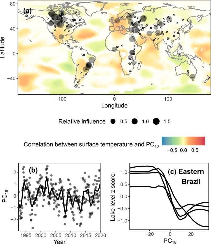
2594                    B. M. Kraemer et al.: Worldwide lake level trends and responses to background climate variation

level in the Aral Sea dropped by 2 m in the first decade fol-       generalize about which regions are most strongly influenced
lowing the onset of irrigation, and continued to decline as         by background climate variation. Our overall goal is to bet-
water use in the watershed intensified. In this case, attribu-      ter understand the impact of large-scale background climate
tion of water level variation to human activity was robust          forcing on lakes in ways that will help communities manage
because an abrupt change in surface water management co-            the benefits derived from lakes in the face of global climate
incided with a comparably abrupt change in the water level          dynamics and anthropogenic influences.
of downstream lakes. However, attributing water level varia-
tion to human activity is more difficult when anthropogenic
effects are subtle relative to the effects of background cli-       2     Methods
mate variation (Corti et al., 1999). This challenge is espe-
cially salient when attributing water level variation to anthro-    2.1    Overview
pogenic climate change (Hassanzadeh et al., 2012; Rodell et
al., 2018), especially at the global scale (Rodell et al., 2018).   The 200 lakes included in our study contain much of
Indeed, there is an ongoing debate about the global extent          the earth’s liquid surface freshwater and a large propor-
and strength of climate change effects on water level varia-        tion of freshwater biodiversity (Vadeboncoeur et al., 2011).
tion in lakes (Muller, 2018).                                       They span a wide range of lake characteristics includ-
   Climate change can affect water levels through a complex         ing surface area (23 to 377 002 km2 ), catchment area (93
web of forces linking surface temperature with hydrology            to 2 764 126 km2 ), perimeter (62 to 15 829 km), latitude
(Block and Strzepek, 2012; Ramanathan et al., 2001; Rodell          (−50.22 to 66.14◦ N), and elevation (−71 to 5194 m above
et al., 2018). While warming has been observed across the           sea level) (Supplement). All continents were represented ex-
earth’s surface, hydrological responses to warming are highly       cept for Antarctica and Australia. According to the Hydro-
variable, with some areas becoming wetter and others be-            LAKES database (Messager et al., 2016), at least 78 of these
coming dryer (Greve et al., 2014; Rodell et al., 2018; Wang         lakes are reservoirs, and 18 of them have some water level
et al., 2012). However, more than three-quarters of earth’s         regulatory structure such as a dam. The global scope of this
land mass has seen no substantial change in total wetness           analysis builds off similar analyses which aimed to disentan-
or dryness in response to recent climate change (Greve et           gle background climate variation’s influence on lake water
al., 2014; Greve and Seneviratne, 2015). Thus, the effects          levels using smaller numbers of lakes from specific regions
of climate change on water levels may be subtle relative to         (Mercier et al., 2002; Molinos et al., 2015) or specific lakes
background climate variation (Jöhnk et al., 2004), calling for      (Cohn and Robinson, 1975; Stager et al., 2005; Tomasion and
statistical approaches that can effectively account for the ef-     Valle, 2000).
fects of background climate variation. Analyzing water levels          Our first objective was to estimate trends in water levels
from lakes worldwide may be especially helpful in reducing          in this global sample of lakes based on average annual wa-
uncertainty about the potential contribution of background          ter level. Annual water levels were used in the trend analysis
climatic variation to long-term trends.                             instead of raw water levels so that trend residuals would not
   Here, we build off previous studies focused on specific          be serially autocorrelated. We calculated trends using Theil–
lake regions (Clites et al., 2014; Molinos and Donohue,             Sen non-parametric regression using the “zyp” package in
2014; Molinos et al., 2015; Pasquini et al., 2008) and at-          R. Theil–Sen slopes represent the median of slopes derived
tempt to disentangle the effects of background climate varia-       from all pairwise combinations of points in a time series. The
tion from other drivers of water levels in 200 globally dis-        statistical significance of each trend (p value) was calculated
tributed lakes using time series of remotely sensed water           using a bootstrapped one-sample Wilcoxon signed-rank test
levels from 1992 to 2019. We investigate two key areas of           with 1000 repetitions where the input data for the test was the
uncertainty: (1) whether apparent anthropogenic water level         complete list of all slopes derived from all pairwise combi-
trends in specific lakes can be explained by background cli-        nations of points in the time series. The number of pairwise
mate variation and (2) whether trends in water levels can be        slopes used in each repetition of the Wilcoxon signed-rank
detected in specific lakes only after accounting for and re-        test was equal to the number of years of water level data for
moving the influence of background climate variation. We            each lake.
use boosted regression trees (BRTs) as a means of removing             Our second objective was to characterize and account for
the effects of background climate variation on water levels in      the effects of background global climate variation on lake
each lake, enabling us to achieve more robust quantification        water levels. We did this by using BRTs to model water level
of the multi-decadal trends which may or may not be an-             variation in each lake as a function of the year, the month of
thropogenic. This approach differs from other recently pub-         the year, and a large set of global climate indices. We cal-
lished approaches (Chanut et al., 1988; Molinos et al., 2015)       culated the relative importance of each global climate index
in that it allows for nonlinear relationships, high levels of in-   in the models for each lake to assess its sensitivity to dif-
teractions between axes of climate variation, nonstationarity,      ferent axes of background climate variation. We use the par-
and missing data. Finally, we assess patterns across lakes to       tial dependence of water level variation on the year term in

Hydrol. Earth Syst. Sci., 24, 2593–2608, 2020                                         https://doi.org/10.5194/hess-24-2593-2020
B. M. Kraemer et al.: Worldwide lake level trends and responses to background climate variation                                2595

the model to reflect the long-term variation in water levels         tioning of atmospheric rivers, which can also drive lake wa-
that is not attributable to background climate variation. We         ter budgets and water levels (Gimeno et al., 2014; Lorenzo
repeat the Theil–Sen slope calculation and p-value calcula-          et al., 2008). This assumption is empirically well supported
tion based on the partial dependence data for the year term          by studies showing that earth surface air temperature varia-
as an estimate of the long-term trend that is not attributable       tion described by ENSO, PDO, and IOD is strongly associ-
to background climate variation. This remaining variation            ated with water level variation across the globe (Stager et al.,
could be attributable to human activity, though we cannot            2007; Tierney et al., 2013; Wang et al., 2010).
draw causal conclusions or distinguish between the various              Disentangling the direct and indirect effects of earth sur-
aspects of human activity which can affect water levels.             face air temperature variation on water level variation could
   We derived the background global climate indices for each         be done using a reductionist approach, i.e., by constructing
lake’s BRT using principal component analysis (PCA) ap-              lake hydrological budgets with all of the water inputs and
plied to global variation in monthly earth surface air tem-          outputs and modeling the effect of human activity on each
perature data through time. This approach is widely applied          of those fluxes. But, for most lakes in our dataset, we lack
in the climate sciences to global grids of temperature, pres-        the field measurements required to model the forces linking
sure, or rainfall data and is analogous to empirical orthogonal      earth surface air temperature to water level variation for the
function (EOF) analysis (Dommenget and Latif, 2008; Han-             entire 28-year water level time series (Hegerl et al., 2015;
nachi et al., 2009; Kim and Wu, 1999). Temperature time              Stenseth et al., 2003). So instead, we use BRTs which mimic
series at each pixel were included as separate variables in          the complex web of forces linking earth surface air tempera-
the PCA with each time step as a separate observation of             ture variation to water level variation. We use BRTs for this
those variables. We linearly detrended temperature variation         purpose because the model structure accommodates high lev-
at each pixel such that the temperature values were equivalent       els of interactions among predictor variables and mimics the
to the residuals from a Theil–Sen regression through time.           interactive and indirect effects we tried to capture. This ap-
Temperatures were detrended because long-term tempera-               proach also differs from other recently published approaches
ture trends could be considered potentially related to anthro-       (Chanut et al., 1988; Molinos et al., 2015) in that it allows
pogenic climate change, which we wanted to separate from             for nonlinear relationships, nonstationarity, and missing data.
the principal components (PCs) representing background cli-          We fit BRTs separately for each lake because the influence of
mate (Stenseth et al., 2003). Thus, the effect of all PCs on         a particular climate oscillation could differ across lakes due
water levels in the BRTs were interpreted as the collective          to geographic forcing, orographic forcing, or other local fac-
effects of background surface air temperature variation and          tors (Stenseth et al., 2003). We used backward-elimination
its associated hydrological effects on lake levels.                  variable selection techniques to identify the PCs for each spe-
   Using the PCs was preferred over using the commonly               cific lake that, when fit against a training dataset, performed
recognized climate indices (NAO, ENSO, IOD, etc.) di-                the best when predicting water level variation in a test dataset
rectly in each lake’s BRTs for several reasons. First, many          with which the model had not been fit. Then, we used the re-
commonly recognized global climate indices are correlated,           sulting BRTs to determine the relative importance of differ-
which makes them problematic for simultaneous use as pre-            ent axes of background climate variation separately for each
dictors, whereas the PCs used here are uncorrelated by defini-       lake.
tion. Second, using the commonly recognized global climate
indices alone would miss a substantial amount of variation           2.2   Data
in air temperature that may still drive climate and hydrolog-
ical variation in lakes but is not yet well recognized. Third,       Water level data were acquired from the NASA/CNES
many of the commonly recognized global climate indices are           Topex/Poseidon and Jason satellite missions via the
defined subjectively (e.g., average temperature difference be-       Global Reservoir and Lake Monitoring (G-REALM) project
tween two subjectively defined areas of the ocean), whereas          version 2.3 (Crétaux and Birkett, 2006) and can be
the PCs used here are less subjective.                               obtained from http://www.pecad.fas.usda.gov/cropexplorer/
   Our modeling approach is based on the recognition that            global_reservoir (last access: 24 January 2020). Although
much of the variation in water levels is directly or indi-           these altimeters were developed to map ocean surface height,
rectly driven by global patterns in earth’s surface air tem-         they have also been used to detect water level changes in
perature via the effects of global temperatures on hydro-            lakes (Birkett, 1995). Only a small subset of the world’s
logical fluxes (Dommenget and Latif, 2008). This relation-           lakes can be monitored in this way because the spaceborne
ship is well supported because earth’s surface air tempera-          sensors must pass directly over the lake with sufficient reg-
ture is a key control on earth’s hydrological cycle through the      ularity to produce accurate and complete time series. The
Clausius–Clapeyron relation, which, in turn, drives lake wa-         US Department of Agriculture (USDA) uses these data to
ter budgets and water levels (Christensen et al., 2004; Fowler       monitor water level variation for many inland water bod-
et al., 2007; Nijssen et al., 2001; Tierney et al., 2008). Earth’s   ies globally. The lakes in this study comprise the 200 lakes
surface air temperature may also be a key control on the posi-       with the longest (> 28 years) and highest-temporal-resolution

https://doi.org/10.5194/hess-24-2593-2020                                         Hydrol. Earth Syst. Sci., 24, 2593–2608, 2020
2596                   B. M. Kraemer et al.: Worldwide lake level trends and responses to background climate variation

time series (greatest number of samples per year). Valida-         Research Laboratory. For indices that are not updated to the
tion of satellite altimeter data over inland water bodies is       present, we calculated the correlation over the longest time
typically performed by comparing satellite altimeter mea-          period over which each major climate index was available.
surements and in situ measurements. The root mean squared          Monthly time series of major climate indices were sourced
error of elevation variations derived from the NASA/CNES           from https://www.esrl.noaa.gov/psd/data/climateindices/list/
Topex/Poseidon and Jason-1 satellite missions is typically         (last access: 24 January 2020). In cases where a PC is highly
∼ 5 cm for large lakes based on the USDA G-REALM web-              correlated to one of the major climate indices (PCs), we re-
site (https://ipad.fas.usda.gov/cropexplorer/global_reservoir/     named it with a subscript (e.g., PCENSO ) to facilitate inter-
validation.aspx, last access: 24 January 2020). Thus, it is jus-   pretation. In all remaining cases, PCs were named with a nu-
tifiable to use altimetry water level observations in place of     meric subscript which matched their order in the PCA (e.g.,
in situ gauge measurements (Birkett et al., 2011).                 “PC18 ”)
    Water levels are typically measured every 10 d, but the ex-
act dates on which water levels are measured vary from lake        2.4   Boosted regression trees (BRTs) and model
to lake. To make water level data temporally consistent, we              selection
linearly interpolated each lake’s time series to the daily scale
using the “deseasonalize” and “zoo” packages in R (R Core          BRTs were used to model mean monthly water levels in the
Team, 2017). Monthly averages were calculated so that all          lakes as a function of year, the month of the year, and a
lakes had time series of the same interval that also matches       large set of PCs. A BRT is an ensemble machine learning
the temporal resolution of surface air temperature data used       approach that differs from conventional statistical techniques
in the PCA. Seventy of the 200 water level time series had         which use a single parsimonious model. Instead, BRTs com-
a data gap from late 2002 through the middle of 2008. The          bine the strengths of standard regression trees and boosting
missing data were not estimated; instead, our analyses treated     – a method for aggregating many models to improve the pre-
these lakes in the same way as lakes with complete data.           dictive capacity. The main advantages of BRTs over other
    Monthly average land and ocean surface air temperature         statistical models are that they have higher predictive perfor-
anomaly data were acquired from the Goddard Institute for          mance, do not require data transformation or outlier elimina-
Space Studies (GISS) land–ocean temperature index analy-           tion, automatically handle complex nonlinear relationships
sis for a 2 × 2◦ grid with 1200 km smoothing (Hansen et al.,       and interactions, and allow for many types of predictor vari-
2010). These temperature data are derived from meteorolog-         ables and partial missing data. Through these interactions,
ical station observations distributed across the globe and pro-    the BRT allows for nonstationarity of the times eries (e.g.,
cessed according to methods developed at the National Aero-        the effect of each PC is allowed to change over time). We
nautics and Space Administration (NASA) (Hansen et al.,            fit BRTs using the “dismo” and “gbm” packages (Hijmans
2010). They are publicly available at https://data.giss.nasa.      et al., 2017) in R (R Core Team, 2017). To cross-validate
gov/gistemp/ (last access: 24 January 2020).                       the BRTs for each lake, we fit the model using a training
                                                                   dataset and then used the fit BRT to predict monthly water
2.3    Principal component analysis                                levels using the PC values from a test dataset. For each lake,
                                                                   we fit six starting models using six different training and test
We used PCA to distill the spatial complexity of surface air       dataset combinations. To get these dataset combinations, we
temperatures for inclusion in each lake’s BRT. PCA is an           first split the lake level time series for each lake into training
ordination-based statistical tool that converts potentially cor-   and test datasets along its time series using 40–60, 50–50,
related variables into a set of orthogonal vectors that capture    and 60–40 splits. We split the data serially along the time
the variation across locations. PCA uses orthogonal linear         series into training and test datasets instead of by randomly
transformation to identify vectors that account for as much        selecting observations for the training and test datasets be-
of the total variation in a set of variables as possible. The      cause the data are temporally autocorrelated and we wanted
first PC (PC1 ) explains the largest percentage of the varia-      to ensure that the training and test datasets were independent.
tion in the underlying set of variables, followed by the second    For each of the three splits, the starting model was fit twice,
(PC2 ), third (PC3 ), and so on. Each succeeding PC is linearly    once using the first part of the split as a training dataset and
uncorrelated to the others and accounts for as much of the         the second part as a test dataset, and once using the second
remaining variation as possible. PCA can, therefore, be used       part of the split as a training dataset and the first part as a test
to summarize the consistent aspects of time dynamics across        dataset, resulting in a total of six train–test dataset combina-
space and reduce redundant spatial variation (stemming from        tions. For each lake’s six train–test dataset combinations, we
spatial autocorrelation and teleconnections) in temperature.       repeatedly refit the starting model after dropping the PC with
   To identify which known oscillations in surface air tem-        the lowest relative importance averaged across all six train–
perature are related to individual PCs, we calculated a com-       test dataset combinations (see explanation of relative impor-
plete correlation matrix between each PC and all of the 43         tance below) until the starting model had only two predic-
major climate indices recognized by NOAA’s Earth System            tors – the minimum number of predictors allowed in a BRT.

Hydrol. Earth Syst. Sci., 24, 2593–2608, 2020                                        https://doi.org/10.5194/hess-24-2593-2020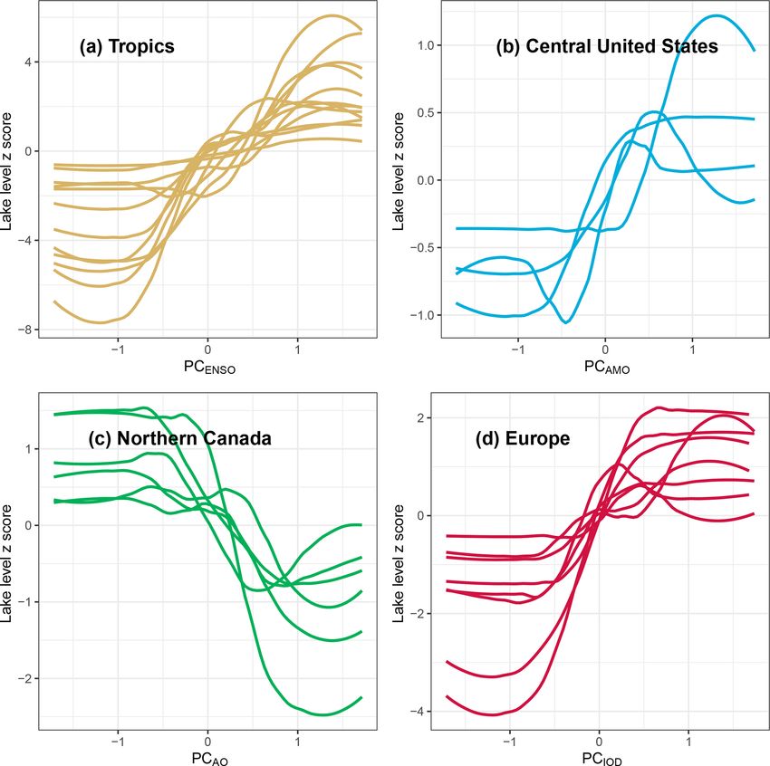
B. M. Kraemer et al.: Worldwide lake level trends and responses to background climate variation 2597
Each time a variable was dropped from one of the six start- in the Middle East and the southwest United States tended to
ing models, we calculated the average change in predicted have decreasing water levels (Fig. 2). Lakes in Canada and
residual error sum of squares (PRESS; the sum of squares of Europe tended to have weak or increasing water level trends.
the prediction residuals calculated using the test data) which Water level trends in East Asia and Africa were highly vari-
resulted from dropping it. able from lake to lake (Fig. 2).
Variables which, when dropped from the model, resulted BRTs performed well for most lakes in our cross-
in an average increase in PRESS across the six starting mod- validation and model optimization procedure; the median
els were selected in that lake’s “best BRT”. We combined PRESS of the best model was 7.0 cm (interquartile range:
information across models so that the selection of a variable 3.5–85.7 cm) across lakes. Two lakes with known anthro-
did not depend on the arbitrary decisions of where to split pogenic water level dynamics, both of which are reservoirs
the time series and whether to use the first or second part as on the Mekong River in China, performed poorly in cross-
the training dataset. All 336 PCs were used as predictors at validation because they had water level increases > 50 m as
the beginning of the model selection process because even a result of dam construction in the middle of the time series
very high order PCs can be important variables in a model (Nuozhadu and Xiaowan dams). Across lakes, the best model
(Phinyomark et al., 2015), and many of the high-order PCs included a median of 11 of the 336 PCs (interquartile range:
calculated here were statistically distinguishable from ran- 3–19 PCs) that were fed into our model selection procedure.
dom noise (Supplement). Thus, the best BRT included the One hundred fifty-four out of 336 PCs were never selected in
year, the month, and the combination of PCs from PC1 to any lake, and the overall frequency of inclusion across lakes
PC336 which consistently improved its performance in cross- decreased with PC order (Kendall’s tau = −0.75, p < 0.01).
validation. A maximum of 336 PCs could be calculated from The median percentage of water level variation associated
336 monthly observations of temperature over the 28-year with background climate variation was 58 % (inner quar-
span of the lake level time series. This best combination of tile range: 33–74 %) with an additional 10 % (inner quar-
PCs, specific to each lake, was used for determining the rel- tile range: 4–22 %) explained by seasonal variation and 25 %
ative importance of the variables selected in the best model. (inner quartile range: 13–50 %) explained by the long-term
We refit the best BRT for each lake to the full time series to trend.
calculate the final relative importance values of each PC. The The relative importance of each specific predictor vari-
relative importance of each predictor variable in the model is able varied substantially from lake to lake. Based on the
a function of the frequency with which it was included in the median relative importance values across lakes, the year
BRT’s individual regression trees and the improvement to the and the month most strongly influenced water level vari-
model that resulted from its inclusion (Elith et al., 2008). The ability. PC1 , PC4 , PC5 , and PC6 were the predictor vari-
relative importance of variables that were not selected in each ables with the third (2.6), fourth (1.6), fifth (1.5), and
lake’s best BRT was set to zero. sixth (1.4) highest median relative importance in the best-
performing BRTs (Fig. 3). PC1 was strongly correlated with
the multivariate El Niño index (MEI; Kendall’s tau = 0.68,
3 Results p < 0.01), PC4 was correlated with the Atlantic Multidecadal
Oscillation (AMO; Kendall’s tau = 0.26, p < 0.01), PC5
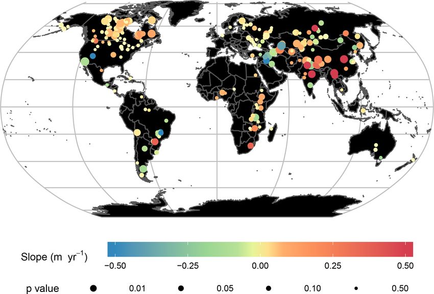
We observed considerable variation in water levels within the was correlated with the Arctic Oscillation (AO; Kendall’s
200 lakes in our analyses (Fig. 1). Prior to accounting for tau = 0.30, p < 0.01), and PC6 was correlated with the In-
the effects of background climate variation, water levels in- dian Ocean Dipole (IOD; Kendall’s tau = 0.21, p < 0.01),
creased at a median rate of 1.2 cm yr−1 (interquartile range: so we renamed them here as PCENSO , PCAMO , PCAO ,
−0.3 to 4.1 cm yr−1 ) (Fig. 1). Water levels were decreasing and PCIOD , respectively (Figs. 3–4). These four PCs to-
in 60 lakes (30 %), of which 14 were statistically significant gether encompass 22.0 % of the variation in surface air
(p < 0.05 level), and increasing in 140 lakes (70 %), of which temperature anomalies according to the eigenvalues from
51 were statistically significant (p < 0.05 level). In total, 65 the PCA (PCENSO = 9.2 %, PCAMO = 5.5 %, PCAO = 4.0 %,
lakes (32.5 %) in our analyses had significant trends in wa- and PCIOD = 3.3 %). PCENSO , PCAMO , PCAO , and PCIOD
ter level (Fig. 1). Given a significance level of α = 0.05, we were selected in the best models for 107, 78, 69, and 70 lakes,
would expect only 10 of our 200 lakes to show “significant” respectively, but the direction of their effects differed among
trends by chance; thus, we observed far more significant lakes (Fig. 3). Many of the remaining PCs of high mean rel-
long-term trends than predicted by chance alone (Fig. 1). A ative importance across waterbodies were only moderately
comparable disparity was observed across a range of differ- correlated to indices from NOAA (Kendall’s correlation co-
ent arbitrary thresholds for statistical significance (i.e., 0.01, efficient < 0.2). For instance, PC18 was not substantially cor-
0.05, and 0.1). related with any climate index recognized by NOAA (maxi-
Changes in water levels from 1992 to 2019 displayed a mum Kendall’s tau = 0.14, p < 0.01) yet exhibited the 11th-
moderate level of regional consistency in the direction and highest median relative importance in explaining water levels
magnitude of water level trends (Fig. 2). In particular, lakes across lakes (Fig. 5).
https://doi.org/10.5194/hess-24-2593-2020 Hydrol. Earth Syst. Sci., 24, 2593–2608, 2020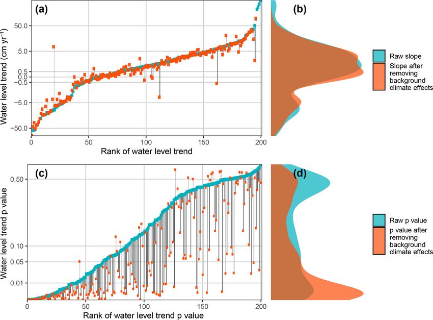
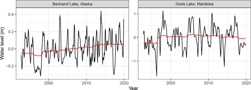
2598                     B. M. Kraemer et al.: Worldwide lake level trends and responses to background climate variation

Figure 1. The change in each lake’s water level trend (a, b) and their trend p value (c, d) which resulted from removing the effects of
background climate variation on water level variation in 200 globally distributed large lakes. After removing the effects of background
climate variation on water levels, long-term water level trend estimates (orange) were slightly more conservative overall compared to rates
calculated from the raw water level data (turquoise). The median value of water level trends across lakes changed from +1.2 to +0.8 cm yr−1
after removing the effects of background climate variation. The trends became more statistically significant in most (86 %, black lines below
the curve) but not all lakes (14 %, gray lines above the curve) after accounting for the effects of background climate variation. The median
p value of water level trends across lakes changed from 0.16 to 0.02 after removing the effects of background climate variation. Lakes are
ranked independently in panels (a) and (c).

   PCENSO , PCAMO , PCAO , and PCIOD were strongly related               lower on average, the trends became more statistically signif-
to water level variation in lakes around the world, but the              icant in 86 % of lakes (Fig. 1). Indeed, the median p value of
strength and directionality of those effects were regionally             water level trends across lakes changed from 0.16 to 0.02
concentrated (Fig. 6). The strongest effects of PCENSO were              after removing the effects of background climate variation
concentrated in the tropics, where it had positive effects on            (Fig. 1). For instance, prior to removing the effects of back-
water levels (Fig. 6). PCAMO was more positively associated              ground climate variation, Becharof Lake in Alaska had an
with water levels in the Midwestern United States and neg-               increasing trend (+0.40 cm yr−1 ) with relatively low statisti-
atively associated with water levels in northern Canada and              cal significance (p value = 0.15). However, after accounting
East Africa. PCAO was also selected in the best models of                for the effects of background climate variation, the trend was
lakes that were regionally concentrated; it was positively as-           not substantially affected (from +0.40 to +0.51 cm yr−1 ) but
sociated with water levels in Central Asia, while it was nega-           became substantially more statistically significant (p value
tively associated with water levels in parts of Canada, Alaska,          from 0.15 to < 0.01). Based on inspection of the time se-
northern Europe, Brazil, and East Africa (Fig. 6). PCIOD was             ries of water levels in Lake Becharof, we suspect that the
positively associated with water levels in Europe (Fig. 6).              strong climate oscillations affecting lake levels throughout
   After removing the effects of background climate variation            the time series, in particular the water level local minima in
on water levels using the fitted BRTs, water level trend esti-           1998 and 2017 as well as the local maxima in 2003 and 2013,
mates were shallower compared to estimates from the origi-               masked the long-term trend (Fig. 7). In contrast, prior to re-
nal time series (Fig. 1). The median water level trend across            moving the effects of background climate variation, Gods
lakes dropped from +1.2 to +0.8 cm yr−1 after correcting for             Lake in Canada had an increasing trend (+1.26 cm yr−1 )
background climate variation (Fig. 1). Even though they were             with a relatively low statistical significance (p value = 0.35).

Hydrol. Earth Syst. Sci., 24, 2593–2608, 2020                                              https://doi.org/10.5194/hess-24-2593-2020
B. M. Kraemer et al.: Worldwide lake level trends and responses to background climate variation 2599
Figure 2. Long-term trends in water levels prior to removing the effects of background climate variation. Some lakes – including those in
the southwest United States, parts of Africa, and the Middle East – show regionally consistent patterns in water levels.
However, after accounting for the effects of background cli- variation masked underlying trends in water levels which
mate variation, the trend flipped sign and was much weaker were detected when the effects of background climate were
(from +1.26 to −0.10 cm yr−1 ) and less statistically signifi- factored out (Supplement Table S2). Thus, attempting to de-
cant (p value from 0.35 to 0.58). Based on inspection of the tect anthropogenic effects on water levels using water level
time series, we suspect that a series of three local water level time series without accounting for background climate varia-
minima early in the lake level time series in 1996, 2000, and tion may over- or underestimate the multi-decadal water level
2004 created a specious appearance of a long-term trend in trends in lakes.
Gods Lake (Fig. 7) that went away when those minima were The trends in water levels estimated here differed widely
attributed to background climate. among lakes, presumably reflecting the heterogeneity of un-
derlying changes in regional hydrological fluxes. Rising wa-
ter levels in the majority of lakes may be attributable to in-
4 Discussion creases in precipitation within their watersheds (Bintanja and
Selten, 2014; Chadwick et al., 2013; IPCC, 2014; O’Gorman
We detected long-term trends in water levels before and after et al., 2012). However, even in watersheds which have expe-
accounting for background climate variation in most lakes in rienced increased precipitation, greater inputs of water may
our analyses. The evidence of trends in the majority of lakes be offset or even exceeded by increases in evapotranspira-
belies reports that most of the earth has experienced no con- tion (Dorigo et al., 2012; Vinukollu et al., 2011; Vörösmarty
sistent changes in annual wetness and dryness (Greve et al., et al., 2000; Vörösmarty and Sahagian, 2006) that yield net
2014; Greve and Seneviratne, 2015). This contrast highlights decreases in water levels.
the potential for waterbody surface levels to serve as integra- Not all of the lakes with significant trends in water lev-
tive metrics of regional water budgets, thereby enhancing our els followed the “wet gets wetter and dry gets dryer” pat-
ability to detect hydrological changes. tern that is often predicted to occur with climate change
Background climate variation had significant effects on (Wang et al., 2012). According to such predictions, surface
water levels in most large lakes between 1992 and 2019. In- water storage would be expected to decrease in many dry
frequently, the effects of multiple axes of background climate mid-latitude and subtropical regions, and to increase at high
variation gave rise to the appearance of long-term trends latitudes and in humid mid-latitude regions (IPCC, 2014).
which became less significant once background climate vari- Several lakes with the strongest decreases in water levels
ation was factored out. But more often, background climate
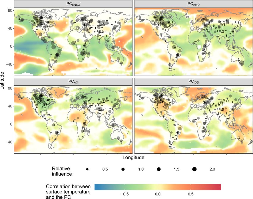
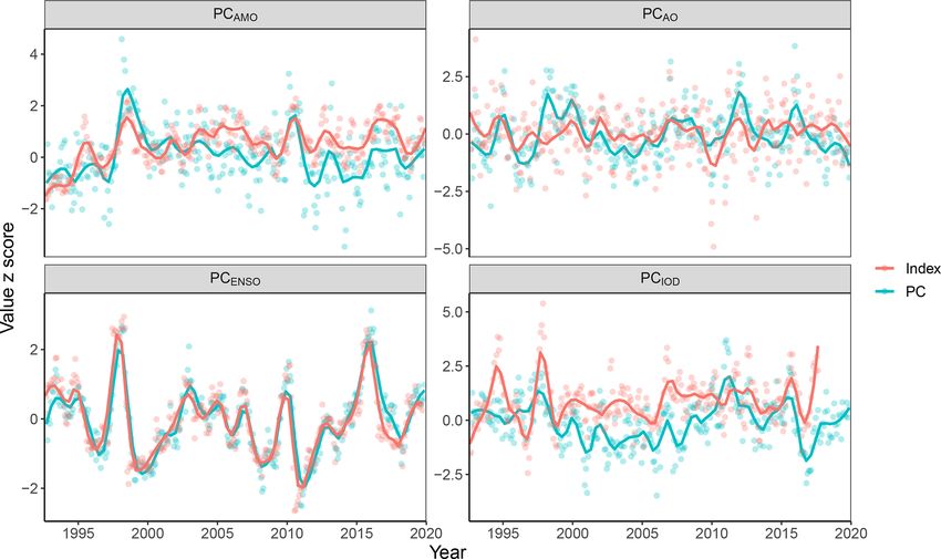
https://doi.org/10.5194/hess-24-2593-2020 Hydrol. Earth Syst. Sci., 24, 2593–2608, 20202600 B. M. Kraemer et al.: Worldwide lake level trends and responses to background climate variation Figure 3. The relative influence of different axes of background climate variation (PCs) on water level variation. Empty dots represent lakes for which the PC was not selected in its “best model”. The opacity of each colored pixel in each map is related to the significance of the correlation between the PC and temperature at that pixel, with less significant correlations appearing white. Figure 4. Time series of background climate variation for the four PCs that were most influential in the best models of water level variation on average across lakes. PCs (PCAMO , PCAO , PCENSO , and PCIOD ) and their corresponding climate indices (AMO, AO, ENSO, and IOD) are transformed to their z scores so that they can be more easily compared on the same unit-less scale. The dots represent raw values, and the lines represent locally weighted scatterplot (LOWESS)-smoothed time series. Hydrol. Earth Syst. Sci., 24, 2593–2608, 2020 https://doi.org/10.5194/hess-24-2593-2020
B. M. Kraemer et al.: Worldwide lake level trends and responses to background climate variation                                        2601

Figure 5. PC18 is an example of a PC which was important for explaining water levels but was not strongly correlated with any of the climate
indices recognized by NOAA. In panel (a), empty dots represent lakes for which PC18 was not selected in its “best model”. The opacity
of each colored pixel in each map is related to the significance of the correlation between the PC and temperature at that pixel, with less
significant correlations appearing white. In panel (b), the dots represent raw values of PC18 , and in panels (b) and (c) the lines represent
LOWESS-smoothed values.

(Aral, Mosul, Powell, Rakshastal, Salton, Tharthar, and Ur-              study, Lake Turkana had a significant increase in water level
mia) are indeed located in relatively dry regions (average               from 1992 to 2019 despite being in a very dry region. Thus,
long-term discharge/watershed area < 5000 cm3 s−1 km−2 ).                intensification of contrasts in precipitation may be a useful
Furthermore, several lakes with the strongest increases in               heuristic for predicting water level trends in some regions
water levels (Zeyaskoye and Atitlán) are located in rela-                but is clearly inapplicable at the global scale (Greve et al.,
tively wet regions (average long-term discharge/watershed                2014; Greve and Seneviratne, 2015).
area > 5000 cm3 s−1 km−2 ). However, the intensification of                 The changes in water levels in response to the four most
wet–dry contrasts was violated in many places as some lakes              important PCs (PCENSO , PCAMO , PCAO , and PCIOD ) often
in wet regions got dryer (Vermelha, Winnebago, and Woods)                matched the direction of change predicted from the hydro-
and some lakes in dry regions got wetter (Balkhash, Cahora               logical changes associated with these particular climate os-
Bassa, Kapachagay, Kariba, and Ulungar). This finding adds               cillations. For instance, we observed strong negative rela-
to others showing that a range of hydrological fluxes con-               tionships between PCENSO and water levels for many water-
tradict the “wet gets wetter and dry gets dryer” pattern over            bodies in sub-Saharan Africa, the equatorial Americas, and
land (Byrne et al., 2015). As a specific example from our                central Canada, as would be predicted based on studies of

https://doi.org/10.5194/hess-24-2593-2020                                              Hydrol. Earth Syst. Sci., 24, 2593–2608, 2020
2602                     B. M. Kraemer et al.: Worldwide lake level trends and responses to background climate variation

Figure 6. Regional consistency in the directionality of PCENSO , PCAMO , PCAO , and PCIOD effects on water level variation. Each line
represents a LOWESS-smoothed relationship between water level variation in a specific lake and one of the four PCs. Water levels have been
transformed into z scores so that they may all be plotted on the same axis.

Figure 7. Water level time series for two North American lakes which show the potential for background climate variation to mask long-term
trends (Becharof Lake) and the potential for climate variation to give rise to the false appearance of long-term trends (Gods Lake). The water
level trend in Becharof Lake in Alaska became more significant after accounting for background climate variation, and the water level trend
in Gods Lake in Manitoba became less significant after accounting for background climate variation. Raw data are shown here, but all trends
were calculated based on annual averages. The black line is the raw water level data, and the red line is the partial dependence of water level
on the year term in the boosted regression trees.

Hydrol. Earth Syst. Sci., 24, 2593–2608, 2020                                               https://doi.org/10.5194/hess-24-2593-2020
B. M. Kraemer et al.: Worldwide lake level trends and responses to background climate variation                             2603

the global effects of ENSO on precipitation (Dai and Wigley,       to background climate PCs themselves in cases where PCs
2000; Ropelewski and Halpert, 1987). We also observed wa-          are highly correlated with human activity. Human water ex-
ter level changes in North America as a function of PCAMO          traction may consistently be a larger proportion of total water
that are consistent with predictions from observed regional        fluxes during certain phases of the ENSO cycle, for exam-
changes in rainfall associated with AMO (Wang et al., 2017).       ple. In the BRTs, this aspect of anthropogenic water level
However, we also detected relationships between water lev-         variation would have been captured by PCENSO rather than
els and PCs that were not consistent with the known hydro-         the year term and would have been erroneously attributed to
logical effects of the ENSO, AO, AMO, and IOD. For exam-           background climate variation. However, if the correlation be-
ple, we found that PCAO had a strong effect on water levels        tween human water extraction and ENSO changed over time,
in East Africa, where the AO is not typically considered to        it would be correctly attributed to the year variable in the
be a major driver of hydrological fluxes. However, the cor-        BRTs, in general accordance with our simplified interpreta-
relation between PCAO and the AO was relatively weak, so           tions.
the apparent influence of PCAO could be driven by climate             Third, we distinguish between anthropogenic climate
variation that was captured by PCAO and not the actual AO          change and background climate variation in our interpreta-
index.                                                             tions because background climate indices like those used
   Fifty-eight percent of the explained variation in water lev-    here are generally considered to be modes of natural vari-
els (median across lakes) could be attributed to large-scale       ation. However, human activity may influence background
climate drivers as represented by the 336 PCs derived from         climate variation as well, perhaps making certain phases of
air temperature records. We included higher-order PCs be-          various climate oscillations more likely (Cai et al., 2015;
cause they might have accounted for additional variation           Capotondi and Sardeshmukh, 2017; Timmermann et al.,
in water levels. But we note that higher-order PCs encom-          1999). We partially accounted for this by removing any lin-
passed far less of the variation in surface air temperatures,      ear trend through time in temperature prior to the PCA. De-
and they were included in far fewer of the lakes’ best wa-         trending the temperature data in this way helped to sepa-
ter level models, so their implications for water levels are far   rate the background climate indices from any ongoing cli-
weaker. For example, PC100 explained only 0.1 % of varia-          mate change. However, more complex interactions between
tion in global surface air temperatures and was included in        climate change and background climate variation would not
our best-performing model for four lakes, albeit with very         be removed by this approach, as in a scenario where climate
low explanatory contribution in those cases. Thus, exclud-         change enhances both positive and negative phases of back-
ing high-order PCs is unlikely to lead to substantial improve-     ground climate oscillations yet has no impact on trends of the
ments or changes to our conclusions. The performance of the        mean. Research on such complex relationships is still incon-
BRTs might be improved by including lag effects (Hansen et         clusive (Allen and Ingram, 2002; Cane, 2005; Collins, 2000;
al., 1998; Hidalgo and Dracup, 2003). However, the compu-          Guilyardi et al., 2009; van Oldenborgh et al., 2005), so we
tation time required to include lag effects was prohibitive.       performed only linear detrending of PCs. We also recognize
   Our interpretations of the statistical patterns reported        that our 28-year time series could also reflect longer-period
herein require several caveats. First, there is substantial de-    climate oscillations such as the Pacific Decadal Oscillation,
bate over which aspect of human activity (e.g., climate            but the limited duration of altimeter-based satellite monitor-
change, land use change, or dam construction/management)           ing of lake levels precludes testing for such influences.
is most important for driving water levels (Gyau-Boakye,              The lakes represented in our study comprise a substan-
2001; Lenters, 2001; Mercier et al., 2002; Ricko et al., 2011;     tial portion of the global liquid surface freshwater on the
Wurtsbaugh et al., 2017). Our modeling approach does not           planet. Our study includes the 10 most voluminous fresh-
discern whether the trends we calculated are anthropogenic         water lakes on earth’s surface (Baikal, Tanganyika, Superior,
or which aspects of human activity are driving water level         Michigan, Huron, Malawi, Victoria, Great Bear, Ontario, and
trends. Hence, future work is needed to disentangle the vari-      Great Slave), which collectively contain more freshwater (to-
ous anthropogenic forces which may influence water levels.         tal 80 241 km3 ) than has been withdrawn from the environ-
Detecting anthropogenic water level trends and distinguish-        ment by humans at the global scale over the last 20 years
ing between the effects of different aspects of human activity     (Food and Agriculture Organization of the United Nations,
on water levels could be achieved by including water level         2016). But the lakes in this study are not representative of
dynamics in earth system models. To date, lake ecosystems          all lakes, which tend to have smaller surface area and shal-
are generally oversimplified in such models, in which lakes        lower maximum depths on average. Thus, the relative impor-
are often assumed to be relatively static, inert bodies on the     tance of background climate oscillations in the remainder of
landscape.                                                         lakes other than the 200 large lakes studied here over the last
   Second, we interpreted the trend in the partial dependence      28 years remains uncertain and should be investigated fur-
values for the year term in each lake’s BRT as being poten-        ther.
tially anthropogenic. However, we cannot exclude the possi-           Our modeling approach could be widely applied to dis-
bility that anthropogenic water level variation was attributed     entangle the effects of background climate on other hydro-

https://doi.org/10.5194/hess-24-2593-2020                                       Hydrol. Earth Syst. Sci., 24, 2593–2608, 2020
2604                   B. M. Kraemer et al.: Worldwide lake level trends and responses to background climate variation

logical changes, including streamflow and pan evaporation         tion on a wide variety of environmental variables, including
rates. The novel statistical method presented here using BRTs     fires, floods, heat waves, and droughts. Tests for long-term
could be used to describe or factor out the effects of long-      trends in environmental variables which may or may not be
term variation in background climate variation on a wide va-      anthropogenic will likely benefit from prior isolation and re-
riety of environmental variables, including fires, floods, heat   moval of the effects of background climate variation using
waves, and droughts – all of which have been shown to be          this method.
sensitive to climate teleconnections (Chen et al., 2016; Lau
and Kim, 2012; Stenseth et al., 2003). Instead of using com-
mon climate indices, we encourage the use of the complete         Code availability. All code used in the production of this paper,
set of PCs calculated here, because important climate oscil-      including data analysis and figures, are published in the Zenodo on-
lations could otherwise be missed. To illustrate this point,      line repository with DOI https://doi.org/10.5281/zenodo.3363187
the PC with the 11th-highest median relative importance in        (Kraemer, 2019).
explaining water level variation was not strongly correlated
with any of the reported NOAA climate indices (Fig. 5).
                                                                  Data availability. Water level data products are courtesy of the
   Wherever water levels are affected by background cli-
                                                                  USDA/NASA G-REALM program, which can be found at https:
mate and human activity, there is the potential to affect lake
                                                                  //www.pecad.fas.usda.gov/cropexplorer/global_reservoir/ (United
ecosystems and the benefits that humans derive from them          States Department of Agriculture Foreign Agricultural Service
(Clites et al., 2014). More than 2 billion people live in wa-     and United States National Aeronautics and Space Administration,
ter stressed regions of the world where human demand for          2020). All GISS data can be found at https://data.giss.nasa.gov/
surface freshwater exceeds the available supply (Mekonnen         gistemp/ (United States National Aeronautics and Space Admin-
and Hoekstra, 2016; Vörösmarty et al., 2000, 2010). Meet-         istration Goddard Institute for Space Studies, 2020).
ing the competing demands for surface freshwater, especially
in water-scarce regions and in the face of anthropogenic en-
vironmental change, is a key challenge for society. Our ca-       Supplement. The supplement related to this article is available on-
pacity to disentangle the effects of background climate os-       line at: https://doi.org/10.5194/hess-24-2593-2020-supplement.
cillations on water levels is key to sustaining our freshwa-
ter resources (Clites et al., 2014; Gronewold et al., 2013).
By applying this BRT statistical approach, we partially dis-      Author contributions. BMK designed the study, developed the
entangled the effects of background global climate indices        model code, and performed the analyses. BMK prepared the ini-
                                                                  tial manuscript. BMK, RA, AS, and PBM contributed to the
on water levels. Many of the large lakes in our analyses
                                                                  manuscript’s revision and editing.
were remarkably resilient to long-term changes from 1992
to 2019. Thus, large lakes may be an increasingly important
resource as water scarcity intensifies in the future. Abrupt
                                                                  Competing interests. The authors declare that they have no conflict
changes in water levels in large lakes remain possible due to     of interest.
human activities and climate change, but our analyses sug-
gest that we have not yet observed such changes in many of
earth’s largest lakes.                                            Acknowledgements. The lead author is grateful for support from
                                                                  the IGB Leibniz Institute for Freshwater Ecology and Inland Fish-
                                                                  eries through their international visiting scholars program and from
5   Conclusions                                                   the German Research Foundation within the LimnoScenES project
                                                                  (AD 91/22-1). We are also grateful for financial support from the
On average, water levels in the world’s large lakes are in-       John D. and Catherine T. MacArthur Foundation grants G-108015-
creasing but are highly variable from lake to lake. Back-         0 and G-1609-151200 to Appalachian State University, and for fur-
ground climate variability often masks these long-term            ther support from the Packard Fellowship in Science and Engineer-
                                                                  ing.
trends in water levels and occasionally gives rise to the ap-
pearance of false trends that wane after background climate
variation is factored out. Background climate variation alone
                                                                  Financial support. This research has been supported by the
can explain a large proportion of water level variability in      Deutsche Forschungsgemeinschaft (grant no. AD 91/22-1) and
lakes worldwide due to the strong influence of earth sur-         the John D. and Catherine T. MacArthur Foundation (grant
face air temperatures on lake levels via climate–lake level       nos. G-108015-0 and G-1609-151200).
teleconnections. These findings highlight further opportuni-
ties to investigate the specific mechanisms that couple cli-      The publication of this article was funded by the
mate and lake levels. The novel statistical method presented      Open Access Fund of the Leibniz Association.
here using BRTs could be used to describe or factor out the
effects of long-term variation in background climate varia-

Hydrol. Earth Syst. Sci., 24, 2593–2608, 2020                                       https://doi.org/10.5194/hess-24-2593-2020
B. M. Kraemer et al.: Worldwide lake level trends and responses to background climate variation 2605
Review statement. This paper was edited by Stacey Archfield and tropics, J. Climate, 26, 3803–3822, https://doi.org/10.1175/JCLI-
reviewed by three anonymous referees. D-12-00543.1, 2013.
Chanut, J. P., D’astous, D., and El-Sabh, M. I.: Modelling the Nat-
ural and Anthropogenic Variations of the St. Lawrence Water
Level, in Natural and Man-Made Hazards, 377–394, Springer
Netherlands, Dordrecht, 1988.
References Chen, Y., Morton, D. C., Andela, N., Giglio, L., and Ran-
derson, J. T.: How much global burned area can be fore-
Aladin, N. V., Plotnikov, I. S., Micklin, P., and Ballatore, T.: Nat- cast on seasonal time scales using sea surface temperatures?,
ural Resources and Environmental Issues Aral Sea: Water level, Environ. Res. Lett., 11, 045001, https://doi.org/10.1088/1748-
salinity and long-term changes in biological communities of an 9326/11/4/045001, 2016.
endangered ecosystem-past, present and future, Nat. Resour. Env. Christensen, N. S., Wood, A. W., Voisin, N., Letten-
Iss., 15, 177–183, 2009. maier, D. P., and Palmer, R. N.: The Effects of Cli-
Allen, M. R. and Ingram, W. J.: Constraints on future changes mate Change on the Hydrology and Water Resources of
in climate and the hydrologic cycle, Nature, 419, 224–232, the Colorado River Basin, Clim. Change, 62, 337–363,
https://doi.org/10.1038/nature01092, 2002. https://doi.org/10.1023/B:CLIM.0000013684.13621.1f, 2004.
Benson, L., Linsley, B., Smoot, J., Mensing, S., Lund, S., Stine, S., Clites, A. H., Smith, J. P., Hunter, T. S., and Gronewold, A. D.: Visu-
and Sarna-Wojcicki, A.: Influence of the Pacific decadal oscilla- alizing relationships between hydrology, climate, and water level
tion on the climate of the Sierra Nevada, California and Nevada, fluctuations on Earth’s largest system of lakes, J. Great Lakes
Quaternary Res., 59, 151–159, https://doi.org/10.1016/S0033- Res., 40, 807–811, https://doi.org/10.1016/j.jglr.2014.05.014,
5894(03)00007-3, 2003. 2014.
Benson, L. V., Lund, S. P., Burdett, J. W., Kashgarian, M., Rose, Cohn, B. P. and Robinson, J. E.: Cyclic fluctuations of wa-
T. P., Smoot, J. P., and Schwartz, M.: Correlation of Late- ter levels in Lake Ontario, Comput. Geosci., 1, 105–108,
Pleistocene Lake-Level Oscillations in Mono Lake, California, https://doi.org/10.1016/0098-3004(75)90010-2, 1975.
with North Atlantic Climate Events, Quaternary Res., 49, 1–10, Collins, M.: Understanding uncertainties in the response of ENSO
https://doi.org/10.1006/qres.1997.1940, 1998. to greenhouse warming, Geophys. Res. Lett., 27, 3509–3512,
Bintanja, R. and Selten, F. M.: Future increases in Arctic precipita- https://doi.org/10.1029/2000GL011747, 2000.
tion linked to local evaporation and sea-ice retreat, Nature, 509, Corti, S., Molteni, F., Palmer, T. N., Corti, S., and Molteni,
479–482, https://doi.org/10.1038/nature13259, 2014. F.: Signature of recent climate change in frequencies of nat-
Birkett C., Reynolds C., Beckley B., and Doorn B.: From Research ural atmospheric circulation regimes, Nature, 398, 799–802,
to Operations: The USDA Global Reservoir and Lake Monitor, https://doi.org/10.1038/19745, 1999.
in: Vignudelli S., Kostianoy A., Cipollini P., and Benveniste, J., Crétaux, J.-F. and Birkett, C.: Lake studies from satellite
Coastal Altimetry, Springer, Berlin, Heidelberg, 2011. radar altimetry, Comptes Rendus – Geosci., 338, 1098–1112,
Birkett, C. M. C.: The contribution of TOPEX/POSEIDON to the https://doi.org/10.1016/j.crte.2006.08.002, 2006.
global monitoring of climatically sensitive lakes, J. Geophys. Crétaux, J.-F., Abarca-del-Río, R., Bergé-Nguyen, M., Arsen,
Res., 100, 25179–25204, https://doi.org/10.1029/95JC02125, A., Drolon, V., Clos, G., and Maisongrande, P.: Lake Vol-
1995. ume Monitoring from Space, Surv. Geophys., 37, 269–305,
Block, P. and Strzepek, K.: Power Ahead: Meeting Ethiopia’s https://doi.org/10.1007/s10712-016-9362-6, 2016.
Energy Needs Under a Changing Climate, Rev. Dev. Econ., Dai, A. and Wigley, T. M. L.: Global patterns of ENSO-
16, 476–488, https://doi.org/10.1111/j.1467-9361.2012.00675.x, induced precipitation, Geophys. Res. Lett., 27, 1283–1286,
2012. https://doi.org/10.1029/1999GL011140, 2000.
Byrne, M. P., O’Gorman, P. A., and O’Gorman, P. A.: The Dommenget, D. and Latif, M.: Generation of hyper
response of precipitation minus evapotranspiration to cli- climate modes, Geophys. Res. Lett., 35, L02706,
mate warming: Why the “Wet-get-wetter, dry-get-drier” scal- https://doi.org/10.1029/2007GL031087, 2008.
ing does not hold over land, J. Climate, 28, 8078–8092, Dorigo, W., de Jeu, R., Chung, D., Parinussa, R., Liu, Y.,
https://doi.org/10.1175/JCLI-D-15-0369.1, 2015. Wagner, W., and Fernández-Prieto, D.: Evaluating global
Cai, W., Santoso, A., Wang, G., Yeh, S. W., An, S. Il, Cobb, K. M., trends (1988–2010) in harmonized multi-satellite sur-
Collins, M., Guilyardi, E., Jin, F. F., Kug, J. S., Lengaigne, M., face soil moisture, Geophys. Res. Lett., 39, L18405,
Mcphaden, M. J., Takahashi, K., Timmermann, A., Vecchi, G., https://doi.org/10.1029/2012GL052988, 2012.
Watanabe, M., and Wu, L.: ENSO and greenhouse warming, Nat. Elith, J., Leathwick, J., and Hastie, T.: A working guide to boosted
Clim. Chang., 5, 849–859, https://doi.org/10.1038/nclimate2743, regression trees, J. Anim. Ecol., 77, 802–813, 2008.
2015. Food and Agriculture Organization of the United Nations: AQUA-
Cane, M. A.: The evolution of El Niño, past and STAT, available at: http://www.fao.org/nr/water/aquastat/main/
future, Earth Planet. Sc. Lett., 230, 227–240, index.stm (last access: 11 July 2018), 2016.
https://doi.org/10.1016/j.epsl.2004.12.003, 2005. Fowler, H. J., Blenkinsop, S., and Tebaldi, C.: Linking climate
Capotondi, A. and Sardeshmukh, P. D.: Is El Niño re- change modelling to impacts studies: recent advances in down-
ally changing?, Geophys. Res. Lett., 44, 8548–8556, scaling techniques for hydrological modelling, Int. J. Climatol.,
https://doi.org/10.1002/2017GL074515, 2017. 27, 1547–1578, https://doi.org/10.1002/joc.1556, 2007.
Chadwick, R., Boutle, I., and Martin, G.: Spatial patterns of precip-
itation change in CMIP5: Why the rich do not get richer in the
https://doi.org/10.5194/hess-24-2593-2020 Hydrol. Earth Syst. Sci., 24, 2593–2608, 2020You can also read