Paleoceanographic changes in the Northern East China Sea during the last 400 kyr as inferred from radiolarian assemblages (IODP Site U1429) ...
←
→
Page content transcription
If your browser does not render page correctly, please read the page content below
Matsuzaki et al. Progress in Earth and Planetary Science             (2019) 6:22
https://doi.org/10.1186/s40645-019-0256-3
                                                                                                                               Progress in Earth and
                                                                                                                                  Planetary Science

 RESEARCH ARTICLE                                                                                                                               Open Access

Paleoceanographic changes in the
Northern East China Sea during the last 400
kyr as inferred from radiolarian
assemblages (IODP Site U1429)
Kenji M. Matsuzaki1,2* , Takuya Itaki3 and Ryuji Tada1

  Abstract
  The East China Sea (ECS) is a shallow marginal sea that is sensitive to glacio-eustatic sea-level changes and is
  influenced by warm oligotrophic water of the Kuroshio Current (KC), the nutrient-rich Taiwan Warm Current, and
  freshwater discharges from rivers in southern China during the East Asian summer monsoon season. In this area, local
  paleoceanographic changes for times prior to 40 ka remain poorly studied because of high sediment accumulation
  rates on the seafloor. During Integrated Ocean Drilling Program Expedition 346, long sediment cores representing the
  last 400 kyr were retrieved from the northern part of the ECS (Site U1429). In these cores, radiolarians are abundant and
  well-preserved, thus using the ecological properties of radiolarians, we analyzed how glacio-eustatic sea-level variations
  have influenced the paleoceanography of the ECS over the last 400 kyr, with a focus on changes in water properties at
  intermediate depths. Additionally, the summer sea surface temperature (SST) and intermediate water temperature at
  about 500 m were quantified by means of data on selected radiolarian species. The KC influenced the shallow water at
  Site U1429 during each interglacial period over the last 400 kyr (marine isotope stages [MISs] 1, 5, 7, 9, and 11), causing
  a high summer SST (about 27 °C), although inflow of the KC into the ECS was probably delayed until after the sea-level
  maximum of interglacial MIS 1 and MIS 5. During this lag time, ECS shelf water was the dominant influence on the
  system. During glacial periods (MISs 2–4, 6, and 10), our data suggest that coastal conditions prevailed, probably
  because of a sea-level drop of more than 90 m. At these times, the summer SST was colder, ca. 20 °C. Changes in the
  relative abundance of Cycladophora davisiana indicate that the most significant changes in the bottom water occurred
  during MIS 6, when the bottom water likely became poorer in oxygen. An increase in the shallow-water primary
  productivity during MIS 7 and MIS 6 was probably the key factor causing the oxygen-poor conditions.
  Keywords: East China Sea, Kuroshio current, Changjiang River, Sea-level variations, Primary productivity, Bottom water,
  Oxygen-poor seawater, Radiolarians

Introduction                                                                          volume of discharge from the Changjiang River increases
The East China Sea (ECS) is a marginal sea of the                                     during the East Asian summer monsoon (EASM), which
Northwest Pacific, and 70% of this sea lies over a contin-                            causes high precipitation in southern China during sum-
ental shelf. The ECS is influenced by warm oligotrophic                               mer and thus triggers greater freshwater discharges from
water of the Kuroshio Current (KC), the nutrient-rich                                 the Changjiang River (e.g., Ichikawa and Beardsley 2002;
Taiwan Warm Current (TWC), and discharges of fresh-                                   Kagimoto and Yamagata 1997; Tada et al. 2016). Thus,
water from the Changjiang River (Chen et al. 1994). The                               the Changjiang River supplies a huge amount of fresh-
                                                                                      water into the northern ECS, and it mixes with the sa-
* Correspondence: km.matsuzaki@aori.u-tokyo.ac.jp
1
 Department of Earth and Planetary Science, Graduate School of Science,
                                                                                      line ambient water influenced by the TWC and KC to
The University of Tokyo, 7-3-1, Hongo, Bunkyo-ku, Tokyo 113-0033, Japan               form the ECS continental shelf water (CSW; e.g., Ichi-
2
 Present address: Atmosphere and Ocean Research Institute, The University             kawa and Beardsley 2002). Moreover, upwelling of the
of Tokyo, 5-1-5 Kashiwanoha, Kashiwa, Chiba 277-8564, Japan
Full list of author information is available at the end of the article
                                                                                      KC subsurface water and the North Pacific Intermediate

                                       © The Author(s). 2019 Open Access This article is distributed under the terms of the Creative Commons Attribution 4.0
                                       International License (http://creativecommons.org/licenses/by/4.0/), which permits unrestricted use, distribution, and
                                       reproduction in any medium, provided you give appropriate credit to the original author(s) and the source, provide a link to
                                       the Creative Commons license, and indicate if changes were made.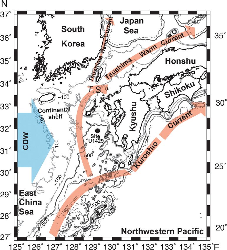
Matsuzaki et al. Progress in Earth and Planetary Science   (2019) 6:22                                                    Page 2 of 21

Water (NPIW) at the slope of the ECS continental shelf                   over the past 20 kyr to monitor and understand the link-
contributes to the availability of a large number of nutri-              age between changes in EASM intensity and ocean re-
ents in the shallow water of the ECS (e.g., Chen 1996;                   sponse at millennial and centennial scales with the goal of
Chen and Wang 1999; Ito et al. 1994; Matsuno et al.                      quantifying and estimating the impact of the precipitation
2009).                                                                   related to the EASM on the local paleoceanography of the
   Global climate during the Pleistocene is known to have                ECS (e.g., Horikawa et al. 2015; Kubota et al. 2010, 2015a).
been characterized by a series of alternating warm and                     One of the concerns is that the paleoceanographic his-
cold (glacial and interglacial) periods, which were regu-                tory of the ECS for periods older than 40 kyr is poorly
lated and paced by the Milankovitch cycles, and signals                  known because even long sediment cores (~ 33.65 m
from these cycles are well-recorded in the oxygen isotope                long in Ijiri et al. 2005) only cover the past 40 kyr due to
ratio (δ18O) of benthic foraminifera (e.g., Berger and                   high sedimentation rates (~ 84.125 cm/kyr) in this area
Jansen 1994; Hays et al. 1976; Lisiecki and Raymo 2005;                  (e.g., Ijiri et al. 2005; Huh and Su 1999; Su and Huh
Elderfield et al. 2012). Recently, Elderfield et al. (2012)              2002). Moreover, we still lack information about the
tried to separate the effects of temperature and global ice              changes in intermediate water hydrography of the ECS,
volume on the deep-ocean foraminifera δ18O. The ampli-                   such as the probable influence of the KC subsurface and
tude of the glacio-eustatic sea-level change (120 m, e.g.,               the NPIW on the local paleoceanography. To document
Yokoyama et al. 2001; Xie et al. 1995) are almost similar                hydrographic changes of the subsurface and intermedi-
in glacial-interglacial cycles for the past 700 kyr, except              ate water is not easy in general because most paleocea-
for the MIS7/8 (300 ka). The Pleistocene is also known for               nographic proxies relied on planktic and benthic
being influenced by millennial-scale climatic instability,               foraminifers, which have calcareous skeletons and in-
the so-called Dansgaard-Oeschger (D-O) events, which                     habit only shallow water (< 300 m) and the seafloor, re-
are abrupt climatic changes caused by periodic collapses                 spectively (e.g., Gooday 2003; Fairbanks and Wiebe
of continental ice sheets in the Northern Hemisphere and                 1980; Kuroyanagi and Kawahata 2004). The microfossil
reductions in North Atlantic Deep Water formation (e.g.,                 group of radiolarians is the only abundant group bearing
Bond et al. 1993; Dansgaard et al. 1993; Hodell and                      skeletons composed of amorphous silica (SiO2·nH2O)
Channell 2016; Tada et al. 2018; Wary et al. 2016). These                and inhabiting deep to shallow water depths (e.g., Suzuki
events also caused variations in sea level.                              and Aita 2011; Suzuki and Not 2015). Numerous studies
   Previous studies have shown that the ECS is sensitive to              of radiolarians in the Northwest Pacific and its adjacent
the glacio-eustatic sea-level changes caused by the glacial/             marginal seas have demonstrated the suitability of this
interglacial cycles because most of its surface water lies               microfossil group as a paleoceanographic proxy (e.g.,
above a continental shelf (< 200 m). Indeed, during glacial              Itaki et al. 2007, 2009; Kamikuri et al. 2007; Matsuzaki
periods over the last 40 kyr, about one-half of the ECS                  et al. 2014a, 2018; Okazaki et al. 2004). Recently, Inte-
continental shelf emerged and the mouth of the Chang-                    grated Ocean Drilling Program (IODP) Expedition 346,
jiang River likely migrated southeastward toward the Oki-                which aimed to reconstruct changes in EASM intensity
nawa Trough because of a sea-level drop of ca. 130 m                     since the Pliocene at high resolution, retrieved sediment
(e.g., Ijiri et al. 2005; Kawahata and Ohshima 2004; Tada                cores at Site U1429 in the Danjo Basin of the northern
et al. 2015; Xie et al. 1995). Such changes in the ECS land-             ECS. These cores continuously cover the past 400 kyr
scape probably caused drastic changes in the local and re-               despite the high sedimentation rates in this area (Tada
gional paleoceanography. Several micropaleontological                    et al. 2015; Sagawa et al. 2018).
and geochemical studies have reconstructed changes in                      Therefore, in this study, we reconstructed the hydro-
local hydrography of the shallow water over the past 40                  graphic changes of the intermediate and shallow water
kyr (e.g., Ijiri et al. 2005; Kawahata and Ohshima 2004;                 depths over the past 400 kyr based on the ecological
Ujiie et al. 1991; Ujiié and Ujiié 1999; Xu and Oda 1999).               properties of selected radiolarian species at IODP Site
It was previously thought that during glacial periods, the               U1429. Our objective was to clarify how the orbital
KC did not enter the ECS and was deflected to the east                   parameters and their associated sea-level variations have
side of the Ryukyu Island Arc (e.g., Ujiie et al. 1991; Ujiié            influenced the local and regional hydrography during
and Ujiié 1999). At present, most studies agree that during              the last 400 kyr, with a particular focus on changes at
the Last Glacial Maximum, the KC likely flowed into the                  intermediate water depths.
southern part of the ECS. However, in the northern ECS,
the KC probably shifted southeastward because of a stron-                Oceanographic setting of the study area
ger influence of coastal waters (e.g., Ijiri et al. 2005; Xie et         The surface water of the ECS is influenced by warm, sa-
al. 1995; Xu and Oda 1999). Recently, several geochemical                line water from the KC and TWC (Tomczak and
studies have also tried to estimate changes in summer sea                Godfrey 1994) (Fig. 1). The KC originates from the
surface temperature (SST) and sea surface salinity (SSS)                 North Equatorial Current and transports warm-saline and
Matsuzaki et al. Progress in Earth and Planetary Science     (2019) 6:22                                                              Page 3 of 21

 Fig. 1 Map from Matsuzaki et al. (2016) modified for this study to show the location of site U1429 and the key oceanographic features of the
 study area. CDW means Changjiang diluted water and IODP means Integrated Ocean Drilling Program

oligotrophic water northward. Its flow volume through                      southern ECS water reach maxima of 28 °C and 34‰, re-
the East Taiwan Strait varies seasonally due to the influ-                 spectively (Sun et al. 2005). In contrast, in the northern
ence of the EASM, and the highest flow of 24 Sv (1 Sv =                    part of the ECS, between China and Kyushu Island, the
106 m3/s) is recorded in summer, while lower flow occurs                   SST and SSS are relatively low, 26 °C and 32‰, respect-
in autumn (20 Sv) (e.g., Lee et al. 2001; Kagimoto and Ya-                 ively. This difference is a consequence of the CDW into
magata 1997; Qu and Lukas 2003). In addition, discharge                    the northwestern ECS (Fig. 1; Ichikawa and Beardsley
of freshwater into the northwestern ECS from the Chang-                    2002). The total annual discharge of freshwater into the
jiang River causes the formation of a low-salinity seawater                northwestern ECS from the Changjiang River reaches a
by mixing with the Taiwan Warm Current, the so-called                      maximum in summer (Beardsley et al. 1985). Therefore,
Changjiang river diluted water (CDW) (Fig. 1) (e.g.,                       the SSS and SST of the northern ECS are greatly reduced
Ichikawa and Beardsley 2002). The CDW flows southward                      because of the CDW, which dominates the shallow con-
along the Chinese coast during winter, whereas during                      tinental shelf before being mixed with the warm, saline,
summer, it flows as a southward coastal jet and has a                      oligotrophic water of the KC and TWC in the northeast-
northward spread (e.g., Beardsley et al. 1985). The thick-                 ern ECS (Fig. 1).
ness of the CDW is around 30 m in the middle shelf area,                     The ECS shelf area is one of the most productive mar-
and it has a lower temperature and lower salinity than the                 ine areas of the world because of Changjiang River fresh-
KC surface water (e.g., Isobe and Matsuno 2008). During                    water discharges (9.24 × 10¹¹ m3 year−1) (Tian et al. 1993)
the summer, the SST and SSS of the shallow waters of the                   and upwelling of the KC subsurface water from a water
Matsuzaki et al. Progress in Earth and Planetary Science   (2019) 6:22                                                  Page 4 of 21

depth of 200–300 m near the slope of the ECS continental                 Assemblage analysis
shelf (Wong et al. 1991; Chen and Wang 1999). These                      In this study, we analyzed changes in the radiolarian as-
Kuroshio subsurface waters are known for being rich in                   semblage for 124 samples at about 0.5 to 1.5 m intervals
nutrients such as nitrate (Chen and Wang 1999; Chen et                   between 0 and 180 m CCSF-D. To monitor changes in
al. 1999; Wong et al. 1991). Therefore, the nutrients                    the northern ECS hydrography, changes in radiolarian
brought up from the euphotic zone increases the local pri-               assemblages and absolute abundances were analyzed for
mary productivity (e.g., Chen 1996; Chen et al. 1999). The               a continuum of the past 400 kyr. Additionally, we esti-
contribution of this nutrient upwelling is higher than that              mated the variation in summer SST and intermediate
from the Changjiang and Yellow rivers (e.g., Chen and                    water temperature at a depth of ca. 500 m by applying
Wang 1999). Additionally, in the ECS, when the Kuroshio                  the method proposed by Matsuzaki and Itaki (2017).
subsurface water upwells, although its influence is smaller,             Two types of microscopic slides were mounted: faunal
some studies have suggested that the NPIW probably                       slides (F-slides) and quantitative slide (Q-slides). The
mixes and upwells along the slope of the ECS continental                 first preparation steps were similar for both types of
shelf and also contributes to the formation of                           slide: the 124 samples were freeze-dried, treated with di-
nutrient-rich shallow water (e.g., Chen 1996; Ito et al.                 luted hydrogen peroxide (H2O2) (15%, i.e., 50 ml of
1994). The NPIW is formed in the Okhotsk Sea and is                      H2O2 at a concentration of 30% diluted in 100 ml of
characterized by a salinity between 33.9 and 34.16‰ and                  water) and hydrochloric acid (15%) (40 ml of HCl at a
an oxygen concentrations between 50 and 150 μmol kg−1                    concentration of 35–37% diluted in 100 m of water) to
(e.g., Kaneko et al. 2001; Bostock et al. 2010). This water              remove organic and calcareous matter. The undissolved
mass subducted into and below the thermocline of the                     residue in each sample was sieved through a 45-μm
Kuroshio Extension before it enters subtropical gyres (e.g.,             screen following the method proposed in Tada et al.
Kaneko et al. 2001).                                                     (2015). Once the undissolved residue was washed, we
                                                                         mounted slides following the procedures proposed by
                                                                         Itaki et al. (2009). Then, we examined polycystine radio-
Materials and methods                                                    larians under an optical microscope at magnifications of
Core samples and age model                                               × 100 to × 400 on both types of slide. All radiolarians
In this study, we analyzed sediment core samples col-                    were identified and counted until at least 400 individual
lected from Site U1429 during IODP Expedition 346.                       tests were identified in each sample, or until the sample
Site U1429 is located in the northernmost part of the                    material was exhausted (see the Additional file 1). The
ECS at a water depth of 732 m and coordinates 31°                        identification followed the nomenclature of Itaki (2009),
37.04′ N and 128° 59.85′ E (Tada et al. 2015). This site                 Matsuzaki et al. (2015a), and Zhang and Suzuki (2017).
is located in the southern part of the Danjo Basin, in                   On average, we counted 435 specimens per slide.
the northern part of the Okinawa Trough (Tada et al.                        We used changes in the entire radiolarian assemblage
2015). The cores are about 180 m long and character-                     over time to estimate species diversity because they can
ized by calcareous-nannofossil-rich clay with diatoms                    be used to constrain changes in radiolarian productivity.
and foraminifera (Tada et al. 2015). The retrieved sedi-                 We used the software PAST 3 of Hammer et al. (2001)
ments are heavily bioturbated and contain tephra layers                  to estimate the number of taxa (S), or species richness,
of various thicknesses, ranging from centimeters to                      which is a count of species recorded in each sample; we
decimeters (e.g., Tada et al. 2015; Sagawa et al. 2018).                 also determined the Shannon-Wiener index (H′), which
This sedimentary succession was divided into two litho-                  describes species diversity by accounting for the relative
logic units (A and B) based on sediment composition                      proportion of each species within a sample as follows:
(Tada et al. 2015). However, we did not analyze litho-                                 X
logic unit B because of heavy drilling disturbance and                        H0 ¼       P i lnP i ;
poor recovery. Unit A spans the Holocene to Middle
                                                                         where Pi is the proportion of each species i in the sam-
Pleistocene (0 to 400 kyr) and consists of olive-gray to
                                                                         ple (Shannon and Weaver 1949).
light-greenish calcareous-rich clay with intercalation of
                                                                           We also estimated species dominance (D), which
tephra layers (Tada et al. 2015).
                                                                         ranges from 0 (all taxa are equally present) to 1 (one
   In this study, we used the core composite depth below
                                                                         taxon dominates the community completely), as follows:
seafloor (CCSF-D) scale of Irino et al. (2018). The depths
                                                                                 X
in CCSF-D were then converted to ages (ka) following                         D¼      ðni =nÞ2 ;
the age model proposed by Sagawa et al. (2018), which
relies upon the oxygen isotope stratigraphy of benthic                   where ni is number of individuals of taxon i and n is the
foraminifer tuned to the LR04 benthic stack (Lisiecki                    total number of samples (e.g., Harper 1999). The domin-
and Raymo 2005).                                                         ance is related to the Simpson index (D = 1 – Simpson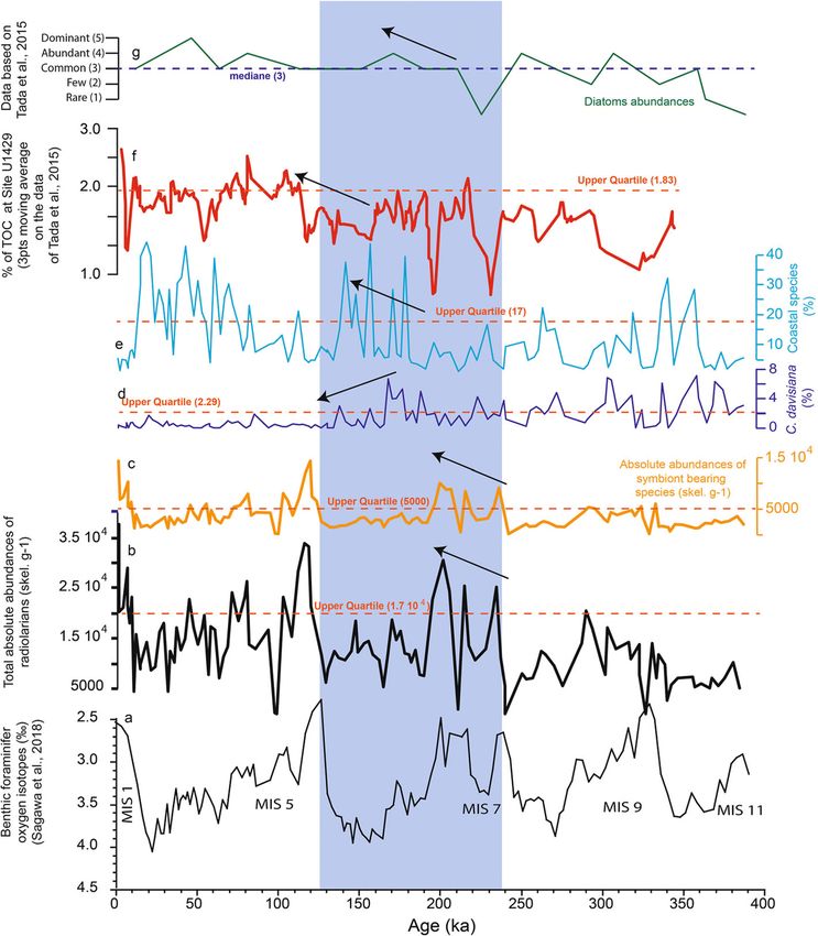
Matsuzaki et al. Progress in Earth and Planetary Science (2019) 6:22 Page 5 of 21
index); however, in this study, the use of D was more assumption was adopted. The selected 17 intermediate
useful for explaining our dataset. water species overlapped with water depths of 500 m, and
From the full assemblage, where 144 species were thus we assumed that intermediate water temperatures re-
identified in 124 samples (see the Additional file 1), we constructed using these selected species corresponded to
selected 45 species with well-known geographic and ver- those of water ca. 500 m deep. Then, intermediate water
tical distributions for reconstructing the paleo-summer temperatures at ca. 500 m provided by the World Ocean
SST and intermediate water temperature following the Atlas were interpolated (i.e., Matsuzaki and Itaki 2017).
nomenclature of Matsuzaki and Itaki (2017). Then, to The relative abundance of the selected species was nor-
reconstruct the regional paleoceanography over the past malized using the procedures of Matsuzaki and Itaki
400 kyr, we selected ten species whose ecology is well (2017). The selected species and their normalized abun-
understood for the ECS based on the findings of Matsu- dances are shown in Additional file 2: Table S1 and
zaki et al. (2016) (Figs. 2 and 3). Additional file 3: Table S2. The SST and intermediate
water temperature were then quantified using the PAST
Sea surface and intermediate water temperature software (Hammer et al. 2001), which implements the
estimation CABFAC and REGRESS routines of the original method
We estimated the SST and intermediate water of Imbrie and Kipp (1971) for Q-mode factor analysis (i.e.,
temperature at a water depth of ca. 500 m by applying Matsuzaki and Itaki 2017).
the method proposed by Matsuzaki and Itaki (2017),
who used the transfer function of Imbrie and Kipp Results
(1971) on a dataset composed of 87 surface sediments Radiolarian absolute abundances
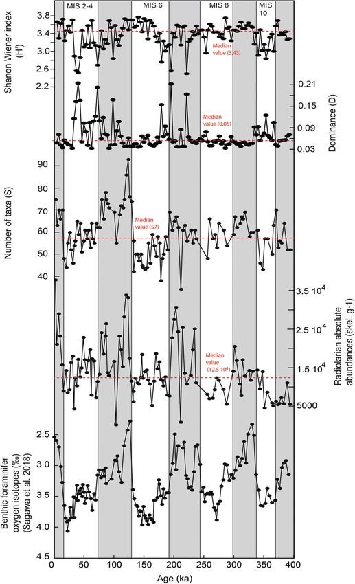
collected in the Northwest Pacific with a particular focus We estimated 1.25 × 10⁴ skel. g−1 to be the median abso-
on the seas surrounding Japan, including the northern lute abundance of radiolarians at Site U1429 (Fig. 4). In
ECS, where more than 20 surface sediment samples were this study, we considered values higher than the median
analyzed [see Matsuzaki and Itaki 2017 for details]. to represent high radiolarian abundance. The interval
Briefly, modern summer SST and intermediate water between 0 and 240 ka, which corresponds to MISs 1–7,
temperature at a water depth of ca. 500 m were attrib- was characterized by high radiolarian absolute abun-
uted to each of the analyzed locations using the World dances. For this period, most of the estimated absolute
Ocean Atlas 2013 (Locarnini et al. 2013) and interpo- abundances were higher than the median and exceeded
lated (with a 1 × 1° grid) onto the geographic position of 2.5 × 10⁴ skel. g−1 during interglacial periods (MISs 1, 5,
each surface sediment station, as detailed in Matsuzaki and 7; Fig. 4). During glacial periods (MISs 2, 4, and 6),
and Itaki (2017). Following the method of Matsuzaki radiolarian absolute abundance was lower than the me-
and Itaki (2017), we selected 28 species living in shallow dian in only a few intervals: at about 20 ka during MIS
water (upper 200 m) for SST estimation and 17 species 2; at about 70 ka during MIS 4; and at about 130 and
living at intermediate water depths for the estimation of 190 ka during MIS 6 (Fig. 4). Therefore, radiolarian
intermediate water temperatures (Additional file 2: Table abundance was generally high between 0 and 240 ka,
S1 and Additional file 3: Table S2). with the highest absolute abundances attained during
For the SST estimates, all the selected species shown warm interglacial periods. In contrast, the time interval
in Additional file 2: Table S1 overlap with a water depth between 240 and 400 ka was characterized by lower
of 0 m (e.g., Matsuzaki et al. 2016; Matsuzaki and Itaki radiolarian absolute abundances (Fig. 4). Most of the
2017; Okazaki et al. 2004). Thus, we assumed that the values in this interval are lower than the median.
reconstructed SST based on these selected shallow-water
species reflect a water depth of 0 m. However, in Radiolarian diversity
Matsuzaki and Itaki (2017), the approach adopted by the We estimated radiolarian diversity by analyzing the full
University of Bremen was used (i.e., http://www.geo.uni-- radiolarian assemblage (the list of taxa is provided in
bremen.de/geomod/ staff/csn/woa-sample.html), which the Additional file 1). We assumed that the number of
integrates the temperature data for the upper 10 m pro- taxa (S) of radiolarian species and species groups can
vided by the World Ocean Atlas. Therefore, the recon- be used as a diversity index. The median number of
structed SST corresponds to an average of the upper 10 m species per sample was 57 (Fig. 4). The species diversity
of the water column. In addition, as shown in Matsuzaki was higher during interglacial periods, with a maximum
and Itaki (2017), we assumed that the reconstructed SST during MIS 5, when the number of radiolarian species
corresponds to the summer SST because the radiolarian exceeded 90 (Fig. 4). Additionally, a drastic increase in
flux is generally low during winter in the Northwest Pa- the number of radiolarian species was recorded at the
cific (e.g., Itaki et al. 2008; Okazaki et al. 2005; 2008). For MIS 5/6 boundary (ca. 130 ka). Before the MIS 5/6
the intermediate water temperature estimates, a similar boundary, the number of radiolarian species (and thus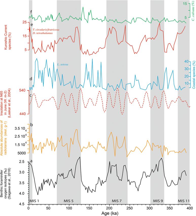
Matsuzaki et al. Progress in Earth and Planetary Science     (2019) 6:22                                                             Page 6 of 21

 Fig. 2 Key Spumellarian species encountered at Site U1429. 1–4 Actinomma leptodermum (Jørgensen) (sample 346-U1429A-7H6-27-29 cm); 5–6
 Actinomma boreale Cleve (sample 346-U1429A-7H6-27-29 cm); 7 Actinomma medianum Nigrini (sample 346-U1429A-1H1-27-29 cm); 8-9 Spongodiscus
 cf. resurgens Ehrenberg (sample 346-U1429A-1H1-27-29 cm); 10-11 Larcopyle weddelium Lazarus, Faust and Popova (sample 346-U1429A-7H6-27-
 29 cm); 12 Spongosphaera streptacantha Haeckel (sample 346-U1429A-1H1-27-29 cm); 14 Druppatractus irregularis Popofsky (sample 346-U1429A-1H1-
 27-29 cm); 15-17 Phorticium polycladum Tan and Tchang (sample 346-U1429A-1H1-27-29 cm); 13 Larcopyle cf. buetschlii Dreyer (sample 346-U1429A-
 7H6-27-29 cm); 18 Tetrapyle circularis Haeckel (sample 346-U1429A-7H6-27-29 cm); 19–21 Tetrapyle fruticosa (Tan and Chen)
 (sample 346-U1429A-7H6-27-29 cm)

the diversity index) was lower than or close to the me-                      We also calculated the species dominance index (D) to
dian value of 57 and never exceeded 70 (Fig. 4). Thus,                     assess the evenness of the radiolarian assemblages
radiolarian diversity was higher between 0 and 130 ka                      (Fig. 4). The median value of D was 0.05 during the past
than between 130 and 400 ka.                                               400 kyr at Site U1429 (Fig. 4). High species dominance
Matsuzaki et al. Progress in Earth and Planetary Science      (2019) 6:22                                                              Page 7 of 21

 Fig. 3 Key Nassellarian species encountered at Site U1429. 1–2 Botryostrobus auritus (Ehrenberg) (sample 346-U1429A-7H6-27-29 cm); 3–5
 Cycladophora davisiana Ehrenberg (sample 346-U1429C-10H4-27-29 cm); 6–9 Arachnocorallium calvata Petrushevskaya group (sample 346-U1429A-
 7H6-27-29 cm); 10, 14 Phormospyris spp. (10. sample 346-U1429C-10H4-27-29 cm, 11 sample 346-U1429A-7H6-27-29 cm); 11–13 Arachnocorys
 castanoides Tan and Tchang (sample 346-U1429A-1H1-27-29 cm); 15–17 Pseudocubus obeliscus Haeckel (sample 346-U1429A-7H6-27-29 cm); 21-24
 Lithomelissa setosa Jørgensen (sample 346-U1429A-7H6-27-29 cm); 18-19 Pseudodictyophimus gracilipes (Bailey) (sample 346-U1429C-10H4-27-29 cm);
 20 Plectacantha oikiskos (Jørgensen) (Sample 346-U1429A-7H6-27-29 cm); 26 Dimelissa thoracites (Haeckel) (sample 346-U1429A-1H1-27-29 cm);
 25 Phormacantha hystrix Jørgensen

is recorded at the MIS 6/7 boundary, with several suc-                      approximately 0.20 (Fig. 4). This result suggests that
cessive values higher than the median (Fig. 4). However,                    during MISs 2–4, the radiolarian assemblage was likely
the highest values of D were recorded between MIS 2                         dominated by a single species, and thus ecological condi-
and late MIS 5, with the maximum value being                                tions enabling this dominance prevailed.
Matsuzaki et al. Progress in Earth and Planetary Science    (2019) 6:22                                                            Page 8 of 21

 Fig. 4 Radiolarian absolute abundance. The number of taxa (S), dominance index (D), and Shannon-Wiener diversity index (H′) are shown over
 time and compared to the benthic foraminifera isotope curve of Sagawa et al. (2018). Red lines indicate median values

  The last species diversity index that we calculated was                 and MIS 11, H′ was close to the median value; however,
the Shannon–Wiener index (H′). The median value of                        between mid-MIS 6 and MIS 1, except for MIS 2, the
this index is 3.43 (Fig. 4). In general, between mid-MIS 6                index value was slightly higher, close to 3.8. This result
Matsuzaki et al. Progress in Earth and Planetary Science   (2019) 6:22                                                    Page 9 of 21

suggests higher species diversity for the mid-MIS 6 to                   cycles, and its relative abundance rarely exceeded 2% of
MIS 1 time interval, except for MIS 2. During intervals of               the assemblage (Fig. 5).
high species dominance (MISs 2–4 and at the MIS 6/7                         The species Lithomelissa setosa Jørgensen (Fig. 5c)
boundary), H′ was at a minimum, with values close                        was almost absent from Site U1429 during interglacial
to 2.6 (Fig. 4).                                                         periods; in contrast, it dominated the radiolarian as-
  In general, the values of the diversity index suggest                  semblages during glacial periods, with relative abun-
that radiolarian species diversity increased after 130 ka                dances greater than 30% of the total assemblage,
(MISs 1 and 5).                                                          except during MIS 8 (Fig. 5). L. setosa is a transi-
                                                                         tional–subarctic species, and it is abundant along the
                                                                         coasts of the Sea of Okhotsk and northeastern Japan
Relative abundances of selected species                                  (e.g., Itaki et al. 2008; Matsuzaki and Itaki 2017). In
We selected ten species or species groups that are useful                the northern Atlantic, L. setosa is dominant in fjord
for reconstructing the paleo-hydrography of the north-                   areas (Bjørklund et al. 1974). Additionally, Itaki et al.
ern ECS over the past 400 kyr from the full radiolarian                  (2008) suggested that this species is probably charac-
assemblage (Fig. 5). Species selection was conducted                     teristic of nutrient-rich coastal areas. Therefore, our
with reference to Matsuzaki et al. (2016): in that study,                data suggest that during MISs 2–4, 6, and 10, Site
radiolarians collected from plankton tows were analyzed                  U1429 was influenced by relatively cold, nutrient-rich
to clarify the regional spatial and vertical radiolarian dis-            coastal water.
tributions (see Matsuzaki et al. (2016) for details). The                   At present, Pseudocubus obeliscus Haeckel (Fig. 5d) is
raw data of the present study are available in the Add-                  an abundant species in the northern ECS (Matsuzaki et
itional file 1.                                                          al. 2016). In our data, this species exhibited higher rela-
   In the northern ECS (Site U1429), the occurrence                      tive abundances, with values close to 10% of the assem-
of the Tetrapyle circularis/fruticosa group (Fig. 5b)                    blage, when the sea level was rising or falling, such as at
sensu Zhang and Suzuki (2017) was high during each                       MIS boundaries (Fig. 5).
interglacial period (i.e., MISs 1, 5, 7, 9, and 11; Fig.                    The species Arachnocorallium calvata Petrushevs-
5). The highest abundance of the T. circularis/fruti-                    kaya (Fig. 5e) is associated with the shallow water of
cosa group (> 22%) was recorded during MIS 9 (300–                       the ECS continental shelf and is probably characteris-
337 ka). Recently, it has been proven that all species                   tic of ECS continental shelf water (Matsuzaki et al.
belonging to the Tetrapyle genus have algal symbionts                    2016). In our data, the relative abundances of A. cal-
and inhabit warm shallow water (Zhang et al. 2018).                      vata were slightly higher for the period between 0
In addition, this species group has been found in                        and 170 ka, for which a relative abundance higher
areas influenced by warm-water currents (e.g., the KC                    than 6% was recorded (Fig. 5).
and its related branches), such as the northern ECS,                        The species Actinomma medianum Nigrini (Fig. 5f)
Japan Sea, and Japan’s Pacific coast (e.g., Lombari and                  exhibited low abundance throughout the core, except
Boden 1985; Itaki et al. 2004, 2007, 2010; Motoyama                      during MIS 10 (337–375 ka), in which the relative abun-
and Nishimura 2005; Kamikuri et al. 2008; Itaki 2009,                    dance of this species exceeded 5% of the total assem-
2016; Boltovskoy et al. 2010; Matsuzaki et al. 2014a,                    blage (Fig. 5). At present, this species is associated with
2015a, 2015b, 2016; Botovskoy and Correa 2016; Mat-                      transitional waters of the Northwest Pacific, where the
suzaki and Itaki 2017). Therefore, the high abundance                    KC and Oyashio Current mix (Matsuzaki and Itaki
of T. circularis/fruticosa during interglacial periods                   2017). This distribution suggests that MIS 10 probably
implies an influence of the KC at Site U1429 (Fig. 5).                   was warmer than other glacial periods. In addition,
Additionally, the maximum abundance of the T. cir-                       Lithomelissa setosa was less abundant during MIS 10
cularis/fruticosa group and its fluctuation pattern                      (Fig. 5), consistent with this interval being warmer.
changed between MISs 6 and 7. For MISs 1 and 5,                             The species group Actinomma boreale/leptodermum
an increase in T. circularis/fruticosa abundance oc-                     sensu Itaki et al. (2004) showed higher relative abun-
curred after a sea-level rise, whereas for MISs 7 and                    dances between 100 and 290 ka, which corresponds to
9, increases in T. circularis/fruticosa abundance were                   MISs 5–9 (Fig. 5h). Two high-abundance peaks (> 20%
almost synchronous with a sea-level rise (Fig. 5).                       of the total assemblage) were recorded during MIS 6 at
   Didymocyrtis tetrathalamus (Haeckel) (Fig. 5g) is also                ca. 140 and 180 ka (Fig. 5). Additionally, the relative
known to inhabit shallow warm water (e.g., Lombari and                   abundance of this species was nearly 10% of the total
Boden 1985; Boltovskoy et al. 2010; Botovskoy and Cor-                   assemblage almost continuously between 190 and 290
rea 2016; Matsuzaki and Itaki 2017). However, at the                     ka (Fig. 5). This species is a subarctic species (e.g., Kling
study site, D. tetrathalamus exhibited no significant vari-              1979; Okazaki et al. 2004; Kamikuri et al. 2008), and in
ations in abundance in response to glacial–interglacial                  the modern ECS, it dominates the assemblage at
Matsuzaki et al. Progress in Earth and Planetary Science (2019) 6:22 Page 10 of 21 Fig. 5 Relative abundances of key radiolarian species encountered at Site U1429 over time, with comparison to the benthic foraminifer isotope curve of Sagawa et al. (2018) intermediate water depths (Matsuzaki et al. 2016). it inhabits shallow to subsurface water depths at However, Pseudodictyophimus gracilipes (Bailey) had higher latitudes (e.g., Kling 1979; Okazaki et al. its highest abundance during MIS 10 (337–375 ka; 2004). High abundances of these species may suggest Fig. 5i). Pseudodictyophimus gracilipes is also a a greater influence of subarctic water at intermediate subarctic species that lives at intermediate water water depths in the ECS from 100 to 290 ka and depths in the ECS (Matsuzaki et al. 2016), although from 337 to 375 ka.
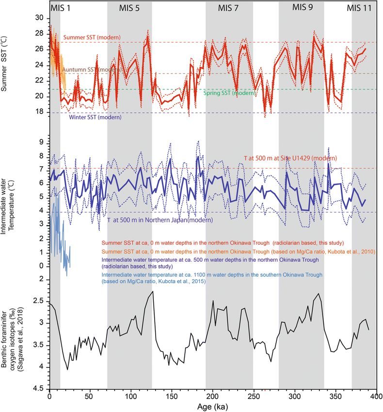
Matsuzaki et al. Progress in Earth and Planetary Science   (2019) 6:22                                                        Page 11 of 21

  The Botryostrobus auritus/australis (Ehrenberg) group                  ECS was likely cold and well ventilated at 160–400
showed high abundance during the earliest stages of MIS                  ka.
9 (300–337 ka), when its relative abundance exceeded
10% of the total assemblage (Fig. 5j). The ecology of this               Summer SST and intermediate water temperature variations
species at that time is largely unknown, but Matsuzaki                   over the past 400 kyr
and Itaki (2017) found that this species is probably related             By applying the dataset and method proposed by Matsu-
to the intermediate water of southern Japan.                             zaki and Itaki (2017), we estimated the paleo-summer
  The abundance of Cycladophora davisiana Ehren-                         SST and intermediate water temperature at ca. 500 m
berg (Fig. 5k) was more than 5% of the total assem-                      based on the selected radiolarian species using the trans-
blage between ca. 160 and 400 ka. The ecology of                         fer function of Imbrie and Kipp (1971) with an error
this species is well understood: its presence implies                    margin of 0.9 °C for paleo-summer SST and 1.2 °C for
cold, oxygen-rich intermediate water (e.g., Boltovskoy                   intermediate water temperature (Fig. 6 and Additional
and Riedel 1987; Kling and Boltovskoy 1995; Okazaki                      file 4: Table S3; see Matsuzaki and Itaki 2017 for
et al. 2003; Itaki and Ikehara 2004; Abelmann and                        details).
Nimmergut 2005; Itaki et al. 2009; Matsuzaki et al.                         Our reconstruction shows that the paleo-summer SST
2014b; Matsuzaki and Itaki 2017). Therefore, our data                    at Site U1429 fluctuated between 18.1 and 28.3 °C, with
indicate that, the intermediate water depth of the                       an error margin of 0.9 °C (Fig. 6). During each

 Fig. 6 Radiolarian-based estimates for intermediate water temperature and SST over time and compared to the benthic foraminifera isotope
 curve of Sagawa et al. (2018). Dashed curves indicate modern median temperatures. Also shown are the summer SST estimated using the Mg/Ca
 ratio of planktic foraminifera (Kubota et al. 2010) in the northern Okinawa Trough and bottom water temperature estimated using the Mg/Ca
 ratio of benthic foraminifera in the southern Okinawa Trough (Kubota et al. 2015b)
Matsuzaki et al. Progress in Earth and Planetary Science   (2019) 6:22                                                   Page 12 of 21

interglacial period, the summer SST exceeded 26 °C, with                 50 m, Kuroyanagi and Kawahata 2004). However, because
a maximum of 28.3 °C at 1.5 ka (MIS 1), whereas during                   the ECS is strongly affected by local and regional influ-
glacial periods, the summer SST was between 18 and                       ences, such as the EASM, which causes freshwater and
22 °C, with a minimum of 18.1 °C at 263 ka (MIS 8; Fig.                  sediment discharges into the ECS, it is also possible that
6). During interglacial periods, our reconstructed summer                the Mg/Ca ratio of foraminifera was influenced by such
SST values are close to the modern summer SST (27 °C)                    factors. To test this hypothesis, the radiolarian-based SST
at Site U1429; the values for glacial periods are between                should be compared again with the SST estimated from
those of modern winter and spring SSTs (17–21 °C;                        Mg/Ca ratios in foraminifera and, if possible, the
Locarnini et al. 2013; Fig. 6).                                          alkenone-based SST in an area less subject to such re-
  The reconstructed intermediate water temperature at                    gional influences, such as the open ocean.
ca. 500 m fluctuated between 3.9 and 8.0 °C, with an error                 We also compared our reconstructed intermediate
margin of 1.2 °C (Fig. 6). These temperatures correspond                 temperature data with those of Kubota et al. (2015b),
to the modern intermediate water temperature at ca.                      who estimated the seawater temperatures at 1100 m
500 m water depth at Site U1429 (ca. 7 °C) and the                       depth in the southern Okinawa Trough from variations
temperature at ca. 500 m off northern Japan (ca. 4 °C;                   in benthic foraminifera Mg/Ca ratios. Our intermediate
Locarnini et al. 2013). The maximum value of 8.0 ± 1.2 °C                water temperature curve fluctuates in a manner similar
was recorded at 180 ka (during MIS 6); the minimum of                    to that of the temperature estimated using benthic
3.9 ± 1.2 °C was recorded at ca. 60 ka (MIS 4; Fig. 6). Al-              foraminifera Mg/Ca over the last 15 kyr (Fig. 6). Al-
though the glacial to interglacial variation is within the               though we note a discrepancy of ca. 3 °C, it can easily be
error range of the method, the reconstructed intermediate                explained by the effect of water depth. Indeed, our
water temperature at ca. 500 m seems to indicate                         temperature estimates correspond to a water depth of
warmer temperatures during interglacial periods and                      ca. 500 m, whereas those of Kubota et al. (2015b) are for
colder temperatures during glacial periods between 0                     water depths of ca. 1100 m, and it is reasonable to rec-
and 130 ka (MISs 1–5; Fig. 6). However, for older                        ord warmer temperatures at shallower depths.
time intervals, there appears to be no correlation with
glacial–interglacial cycles.                                             Evolution of local shallow water over the last 400 kyr
                                                                         The hydrography of the ECS shallow water is sensitive
Discussion                                                               to glacio-eustatic sea-level changes caused by glacial–
Comparison of radiolarian-based summer SST and                           interglacial cycles (Figs. 5, 7, and 8). Based on the paleo-
intermediate water temperatures                                          ceanographic changes inferred from our radiolarian data,
We compared our SST data with the results of Kubota et                   as described in the “Results” section, an overview of ECS
al. (2010), who estimated summer SSTs on the basis of                    shallow-water hydrography during each of the three
variations in the Mg/Ca ratio of the planktic foraminifer                sea-level regimes that have prevailed during the past 400
Globigerinoides ruber (D’Orbigny). The radiolarian-based                 kyr is provided in Fig. 8.
summer SST and Mg/Ca variation-based summer SST are
similar for interglacial periods, confirming the suitability             Evolution of local shallow water during interglacial periods
of our method. However, there are some discrepancies be-                 The fluctuations of the radiolarian-based summer SST
tween the two sets of results for glacial periods (Fig. 6):              curve are generally synchronous with those of the oxy-
radiolarian-based summer SSTs are ca. 2 °C colder than                   gen isotope curve of benthic foraminifera at Site U1429
those inferred from foraminifera. Although there is no                   (Sagawa et al. 2018). The summer SST values were close
clear explanation for this pattern at this time, we                      to the modern summer SST during interglacial periods
hypothesize that for glacial periods, our summer SST                     (ca. 27 °C) (Fig. 6). This increase in SST was caused by
values do not reflect the temperature near the water                     the presence of the KC at Site U1429. Indeed, the radio-
surface but rather the temperature at ca. 100 m. During                  larians Tetrapyle circularis/fruticosa and Didymocyrtis
glacial periods, the dominant radiolarian species was                    tetrathalamus, which are markers of KC water in the
Lithomelissa setosa (Additional file 2: Table S1), which in-             Northwest Pacific (e.g., Lombari and Boden 1985;
habits the subsurface (e.g., Bjørklund et al. 1974; Itaki                Boltovskoy et al. 2010; Hernández-Almeida et al. 2017;
2004; Matsuzaki et al. 2016). Therefore, our glacial-period              Matsuzaki and Itaki 2017), showed relative abundances
SST values may reflect the subsurface sea temperatures,                  higher than 15% during MISs 1, 5, 7, 9, and 11 (Fig. 7).
whereas during interglacial periods, because of the high                 This finding suggests that KC water influenced the shal-
abundances of KC species that prefer the upper 25 m of                   low water of the northern ECS during each interglacial
the water column in the northern ECS (Matsuzaki et al.                   period of the past 400 kyr (Fig. 7). This result is in
2016), it is likely that we obtained information on the part             agreement with previous studies suggesting that the KC
of the environment similar to the habitat of G. ruber (0–                influenced the northern ECS during interglacial periods
Matsuzaki et al. Progress in Earth and Planetary Science (2019) 6:22 Page 13 of 21 Fig. 7 Temporal fluctuation of various radiolarian abundances: a benthic foraminifera isotope curve of Sagawa et al. (2018), b radiolarian absolute abundance, c insolation at 65° N (Paillard et al. 1996), d coastal water species (%), e KC-related species (%), and f continental shelf species (%) (Xie et al. 1995; Xu and Oda 1999; Ijiri et al. 2005; Shi et with maxima of EASM intensity, which causes an increase al. 2014). Our study also demonstrates that the path of in precipitation. Thus, during these maxima, discharges of the KC was probably similar to the modern path during freshwater into the ECS are higher (e.g., Wang et al. 2001, every interglacial period of the past 400 kyr. 2008). Therefore, in the ECS, it is probable that intensifi- However, for MIS 1 and MIS 5, the SST and the cation of the EASM and the related southeastwards relative abundances of KC species increased after the expansion of ECS shelf water weakened the KC inflow that benthic foraminiferal δ18O values reached a low point, passes across the northern ECS at the MIS 1/2 and MIS which indicates a sea-level maximum (Figs. 5 and 7). 5/6 transitions (Fig. 8). Furthermore, the abundance of Arachnocorallium calvata increased at those times (Fig. 7). This species is Evolution of local shallow water during glacial periods known to inhabit the ECS shelf water (Matsuzaki et al. During the last glacial period (MIS 2), the ECS continen- 2016); thus, our data imply that when the sea-level rose tal shelf was exposed, which triggered eastward migra- and reached a maximum, shelf water expanded eastwards tion of the coastlines and river mouths of the main and influenced our study site. Therefore, the KC only in- Chinese rivers (Xie et al. 1995; Xu and Oda 1999; Kawa- fluenced our site and the northern ECS after the rise in hata and Ohshima 2004; Ijiri et al. 2005). However, the sea level. These MIS transitions correspond to maxima of paleoceanography of older glacial periods has remained summer insolation at 65° N. In the ECS, and Asia in gen- unknown because of the lack, until now, of sediment eral, maxima of summer insolation at 65° N are associated cores covering time intervals prior to 40 ka. Based on
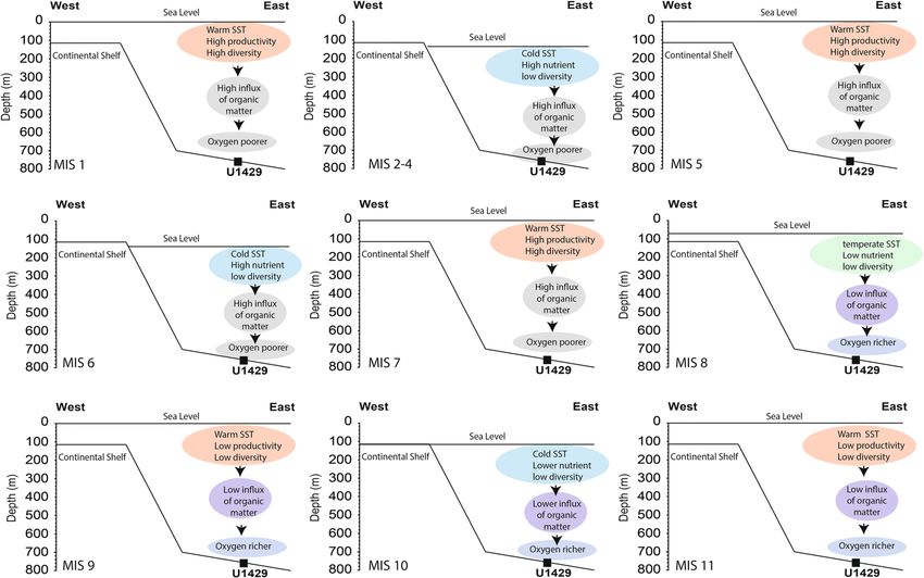
Matsuzaki et al. Progress in Earth and Planetary Science     (2019) 6:22                                                  Page 14 of 21

 Fig. 8 Postulated hydrographic evolution of the northern ECS over the last 400 kyr

our data, the paleoceanographic conditions during MISs                     curve does not show such variability (Fig. 7). During the
2–4, 6, and 10 were likely very similar, although MIS 10                   past 1500 kyr, the climate at high latitudes of the North-
was probably warmer because Actinomma medianum, a                          ern Hemisphere was influenced by millennial-scale D-O
transitional species of the North Pacific, exhibited                       events (e.g., Bond et al. 1993; Dansgaard et al. 1993,
relative abundances of about 5% (Figs. 5 and 7). Thus, a                   Hodell et al. 2016; Tada et al. 2018). These high-latitude
similar sea-level drop probably occurred during MISs 2–                    climate changes likely affected the EASM and paleocea-
4, 6, and 10 (Fig. 8). This scenario is consistent with a                  nography of seas adjacent to Asia, such as the Sea of
recent study that attempted to separate the effects of                     Japan, by influencing the path of the westerly jet (e.g.,
temperature and global ice volume on deep-ocean                            Tada et al. 1999; Tada 2004; Itaki et al. 2007; Kido et al.
foraminiferal δ18O values (Elderfield et al. 2012). The                    2007; Nagashima et al. 2007, 2011; Ikehara and Oshima
radiolarian Lithomelissa setosa, a coastal-water species,                  2009). As argued by Oba et al. (1991) and Tada et al.
dominated the assemblage with relative abundances ex-                      (1999), the ECS is the only source of the surface water
ceeding 40% during these glacial periods (Fig. 7). In the                  in the Sea of Japan. Therefore, the high variability in L.
modern era, L. setosa dominates the coastal environment                    setosa abundance and radiolarian absolute abundance
of northern Japan and is absent offshore (Kamikuri et al.                  recorded at site U1429 was probably related to the influ-
2008; Matsuzaki and Itaki 2017). Additionally, this                        ence of D-O events, but our sampling interval precludes
species is probably associated with nutrient-rich                          further discussion here.
coastal water created by suspension of lithogenic mat-                       The MIS 8 glacial period stands out as different from
ter (Itaki et al. 2008). Therefore, our data suggest that                  other glacial periods during the past 400 kyr. Indeed, al-
during MISs 2–4, 6, and 10, nutrient-rich coastal                          though coastal species dominated during other glacial
water prevailed because of probable higher input of                        periods, during MIS 8, continental shelf species (A. cal-
terrigenous matter and consequent eastward migra-                          vata and Pseudocubus obeliscus) and KC species showed
tion of the coastline.                                                     high abundances during the later and earlier parts of the
  For MISs 2–4 and 6, high variability in Lithomelissa                     stage, respectively (Fig. 7). During early MIS 8, the ben-
setosa abundance and radiolarian absolute abundance                        thic foraminiferal δ18O values were close to those of
are observed, whereas the benthic foraminiferal δ18O                       MIS 5 (Sagawa et al. 2018), suggesting that early MIS 8
Matsuzaki et al. Progress in Earth and Planetary Science   (2019) 6:22                                                  Page 15 of 21

was distinguished by warmer deep water, a smaller                        addition, most of the radiolarian species inhabiting shal-
sea-level drop, or both (Fig. 8). Indeed, the estimates of               low water in tropical to subtropical areas of the NW Pa-
Elderfield et al. (2012) also imply a relatively smaller                 cific bear algal symbionts (Suzuki and Not 2015; Zhang
glacio-eustatic sea-level drop during MIS 8; thus, it is                 et al. 2018). This fact suggests that radiolarians contrib-
probable that the warming recorded during early MIS 8                    ute, in part, to primary ocean productivity, at least in
in the northern ECS was related to the sea level being                   warm areas (De Wever et al. 2001; Suzuki and Not 2015;
slightly higher than during other glaciations. The causes                Zhang et al. 2018). In Fig. 9, we plotted total radiolarian
of this higher sea level are not understood at this time.                absolute abundances and absolute abundances of species
In other areas, unexpected warming was recorded for                      bearing algal symbionts following Zhang et al. (2018).
the northern Japan Pacific coastal areas (off the Shimo-                 Both curves fluctuate in a similar manner, suggesting
kita Peninsula) based on radiolarian data (Matsuzaki et                  that radiolarian absolute abundance is likely related to
al. 2014a), whereas the time interval corresponding to                   ocean primary productivity, at least in warm areas. Add-
MIS 8 is missing (hiatus) from sediment cores retrieved                  itionally, modern observations have indicated that the
at sites C0001 and C0002 during IODP Expedition 315                      maximum radiolarian standing stock occurs at the water
on the Pacific side of the Honshu Island coast off the Kii               depths in which the chlorophyll-a concentration is at a
Peninsula, Japan (Matsuzaki et al. 2015b). In the North-                 maximum (e.g., Kling 1979; Matsuzaki et al. 2016).
west Pacific (Shatsky Rise ODP Site 1209), calcareous                       However, there is a discrepancy between radiolarian
nannofossil data suggest an increase in primary product-                 abundance and other primary productivity indicators
ivity during MISs 8–12 (Bordiga et al. 2013). Addition-                  such as total organic carbon (TOC %) and diatom
ally, planktic foraminiferal and calcareous nannofossil                  abundance (Tada et al. 2015; Fig. 9). The TOC and dia-
data suggest that a modern water-mass structure was                      tom data show that primary productivity at this site did
established in the Northwest Pacific (Shatsky Rise ODP                   not alter in association with glacial and interglacial cy-
1210) at ca. 300 ka (MIS 8; Chiyonobu et al. 2012).                      cles; instead, the primary productivity seems to have
Therefore, MIS 8 appears to have been different from                     changed during the time interval between 130 to 220 ka
other glacial maxima, but this difference cannot cur-                    (Fig. 9). This discrepancy can be explained by consider-
rently be explained based on our data and other avail-                   ing that two factors control ocean primary productivity:
able multi-proxy data available for this stage.                          sunlight and nutrients. Radiolarians related to the KC
                                                                         bear algal symbionts because they inhabit oligotrophic
Evolution of local primary productivity and its consequences             waters and thus have to obtain energy from photosyn-
for bottom water                                                         thesis. This fact explains why the absolute abundances
Evolution of local primary productivity based on radiolarians            of algal-symbiont-bearing radiolarians were higher dur-
Ocean acidification can drastically affect biomineraliza-                ing interglacial periods, and suggests that the absolute
tion by calcareous micro-organisms (e.g., Kawahata et al.                abundances of algal-symbiont-bearing species can be
2018), but such effects are not well understood for                      used as a primary productivity index for interglacial pe-
polycystine radiolarians. Indeed, we just know that the                  riods. However, this index cannot be used to compare
skeletons of polycystine radiolarians are composed of                    primary productivity between interglacial and glacial
amorphous (opaline) silica, and undersaturation of opal                  periods. Indeed, our data show that the KC did not in-
in sea water causes opal to dissolve at the seafloor (e.g.,              fluence our site during glacial periods; thus, the abso-
Takahashi 1981). These observations imply that the ab-                   lute abundances of algal-symbiont-bearing species
solute abundance of radiolarians in sediment is affected                 decreased. In contrast, the percentage abundances of
by changes in both primary productivity and dissolution                  coastal species increased during glacial periods because
at the seafloor. At Site U1429, the preservation of radio-               of the sea-level drop and consequent southeastward mi-
larian skeletons has been reported to be moderate to                     gration of the coastlines and river mouths of the main
good (Tada et al. 2015), which was confirmed by our ob-                  Chinese rivers, which might have led to a marked in-
servations. Specifically, no signs of strong dissolution                 crease in the nutrient levels in shallow water. This find-
were recognized because most species were identifiable                   ing indicates that, although we detected a drastic
and only slight damage to individual specimens was ob-                   decrease in the abundances of species that bear algal
served. Such minor changes in radiolarian preservation                   symbionts, high nutrient levels were available in the
may be related to changes in sedimentation rates be-                     shallow water during glacial periods, and thus the
cause at Site U1429 the sedimentation rates varied from                  ocean primary productivity should have been also high
30 to 40 cm/kyr during interglacial periods to ca. 60–                   during those times. Therefore, to compare and discuss
80 cm/kyr during glacial periods (Sagawa et al. 2018).                   changes in ocean primary productivity during glacial
Therefore, we assume that dissolution is not the main                    periods, abundances of coastal species (such as Litho-
factor regulating radiolarian absolute abundances. In                    melissa setosa) should be used.
Matsuzaki et al. Progress in Earth and Planetary Science (2019) 6:22 Page 16 of 21 Fig. 9 Temporal fluctuation of the local primary productivity: a benthic foraminifera isotope curve of Sagawa et al. (2018), b radiolarian absolute abundance, c radiolarian absolute abundance of species bearing algal symbiosis based on Zhang et al. 2018 (A. vinculata, B. scutum, L. hispida, P. obeliscus, P. praetextum, P. clausus, A. lappacea/spinosa, D. tetrathalamus, D. muelleri, P. pylonium group, S. resurgens, S. streptacantha, Tetrapyle circularis/fruticosa group, L. reticulata, Heliodiscus spp., D. elegans), d C. davisiana (%), e continental shelf species (%), f total organic carbon (TOC) (%), and g diatom abundances In this context, the absolute abundance of radiolarians sea-level drop and/or changes in wind intensity may that bear algal symbionts indicate higher primary prod- have been the cause(s). In contrast, the increase in pri- uctivity for the interglacial periods MISs 1, 5, and 7, but mary productivity during interglacial periods is probably not MISs 9 and 11 (Fig. 9). In contrast, the abundances related to KC dynamics. Previous studies showed that of coastal species were higher during MISs 2–4 and 6 the productivity and nutrient content of the northern than during MIS 8 and 10 (Fig. 9). Combining both ECS are controlled by upwelling of the KC subsurface types of radiolarian data, our results suggest an increase water on the slope of the ECS continental shelf because in local primary productivity from the MIS 6 to MIS 7 this subsurface water is rich in nutrients such as nitrate (130–220 ka). The data on TOC (%) and diatom abun- (Wong et al. 1991; Chen and Wang 1999; Chen et al. dances of Tada et al. (2015) suggest a similar trend, with 1999). Although the mechanism causing upwelling of a higher TOC (%) around late MIS 6 and an increase in KC subsurface water is debated, Chen and Wang (1999) diatom abundance during early MIS 7 (Fig. 9). and Chen (2000) suggested that advection of freshwater The increases in primary productivity during MISs 2– discharged from rivers by estuarine circulation allowed 4 and 6 are difficult to explain, but the amplitude of KC subsurface water to well up to the shelf. This
Matsuzaki et al. Progress in Earth and Planetary Science (2019) 6:22 Page 17 of 21
upwelling supplied nutrients to the continental shelf of Abelmann and Nimmergut 2005; Matul 2011). In the
the ECS, which increased the local primary productivity North Pacific, C. davisiana dominates assemblages in
(e.g., Chen 1996; Chen et al. 1999). Therefore, we areas where the NPIW is formed (young NPIW), par-
hypothesize that local productivity may have been lower ticularly in the northern Japan Oyashio area, where
during MIS 9 than in later interglacial periods because the OSIW mixes with water of the North Pacific (Tal-
of weaker upwelling of KC subsurface water at the slope ley 1993; Yasuda 1997, 2004; Okazaki et al. 2003;
of the ECS. Itaki and Ikehara 2004; Abelmann and Nimmergut
2005; Itaki et al. 2009; Matul 2011; Matsuzaki et al.
Primary productivity and changes in intermediate water 2014b; Matsuzaki and Itaki 2017). In other areas of
oxygenation the North Pacific, particularly at middle to low lati-
The intermediate water of the ECS was probably less tudes, the relative abundance of C. davisiana is much
sensitive than the shallow water to the glacio-eustatic lower, even in areas influenced by the NPIW (e.g.,
sea-level changes forced by orbital parameters. The re- Boltovskoy and Riedel 1987; Kling and Boltovskoy
constructed intermediate water temperature at ca. 1995; Matsuzaki and Itaki 2017). Therefore, we can
500 m was apparently lower for the time interval from assume that C. davisiana is abundant in areas directly
mid-MIS 6 to MIS 11 (> 160 ka) compared to later MISs and/or indirectly influenced by the OSIW and that
(Fig. 6). This finding is based on the occurrence of this species is related to cold, oxygen-rich water
Cycladophora davisiana, which had a relative abundance masses. In addition, based on studies conducted in
of 5% or more of the total assemblage between mid-MIS the modern ECS, C. davisiana generally inhabits
6 and MIS 11, whereas for the interval between MIS 1 water depths below 500 m, although its abundance is
and mid-MIS 6, its relative abundance was approxi- low (< 1.5%; Fig. 10; Matsuzaki and Itaki 2017).
mately 0% (Figs. 5 and 9). Therefore, we can infer that, as our site is ca. 730 m
Previous studies demonstrated that Cycladophora below present-day sea level, the abundance of C.
davisiana dominates the radiolarian assemblage of the davisiana is indicative of the bottom-water environ-
Okhotsk Sea Intermediate Water (OSIW), which has mental conditions. Therefore, our data imply that the
cold, oxygen-rich water masses (Okazaki et al. 2003, bottom water was moderately oxygenated and rela-
2004; Hays and Morley 2004; Itaki and Ikehara 2004; tively cold between 160 and 400 ka, whereas after
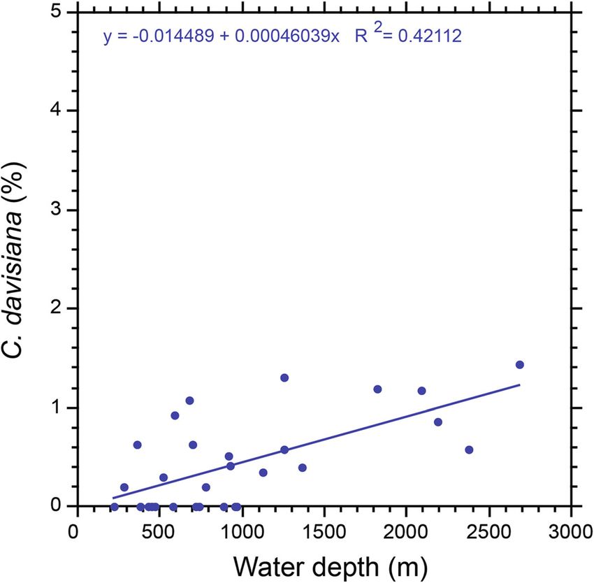
Fig. 10 Current vertical distribution of C. davisiana in the ECS based on the dataset of Matsuzaki and Itaki (2017)Matsuzaki et al. Progress in Earth and Planetary Science (2019) 6:22 Page 18 of 21
than 160 ka, the bottom water was oxygen-poorer Additionally, our data suggest that the shallow water
and also probably warmer (Fig. 7). was likely rich in nutrients due to injection of litho-
Changes in Cycladophora davisiana abundance cannot genic matter into the shallow water precipi1tated by
be explained by plausible changes in the NPIW eastward migration of the Chinese coastline.
influence, because the NPIW is characterized by low 3. The intermediate water temperature at a water
oxygen content in the ECS, and C. davisiana prefers an depth of ca. 500 m reconstructed from our
oxygen-rich environment (e.g., Kaneko et al. 2001). radiolarian assemblages fluctuated roughly
Thus, we attribute changes in bottom-water oxygenation synchronously with the interglacial–glacial period
to local factors. Indeed, from our data and other on- cycle between 0 and 130 ka (MIS 5/6 boundary).
board data of Tada et al. (2015) discussed above, the For older periods, the water temperature at ca.
time interval between MIS 1 and MIS 7 (0–220 ka) was 500 m was probably not related to these cycles.
probably characterized by higher primary productivity in 4. The data on radiolarian assemblages suggest that
shallow waters (Fig. 9). This finding implies that the the bottom-water oxygenation changed at site
deep-sea sediments collected from site U1429 became U1429 around 160 ka. Oxygen-poor conditions ap-
richer in organic carbon after 220 ka (Fig. 9). Therefore, it pear to have prevailed after mid-MIS 6 (ca. 160
is likely that the inferred increase in the primary product- kyr), whereas the interval between mid-MIS 6 and
ivity of shallow waters during MIS 6 and MIS 7 enhanced MIS 11 was relatively richer in oxygen. This change
the production of organic matter (carbon), which sank to was probably caused by increased shallow-water
the sea bottom and increased the amount of organic car- productivity, which resulted in larger amounts of
bon in deep-sea sediments. This organic carbon accumu- sinking organic matter; oxidation of this additional
lated at the seafloor and was oxidized, which consumed organic matter led to increased oxygen
the available oxygen at these depths (e.g., Ruddiman consumption.
2001). Therefore, an increase in the shallow-water prod-
uctivity reduced the amount of available oxygen in the Additional files
bottom water and thus decreased the bottom-water oxy-
genation, which probably caused the lowering of C. davisi- Additional file 1: Counts of radiolarians species at Site U1429 (IODP
ana abundance. 346). (XLSX 118 kb)
Additional file 2: Table S1. Relative abundance (%) of selected shallow
water species after the normalization of Matsuzaki and Itaki (2017) to
Conclusions estimate the paleo-summer SST at site U1429 (PDF 37 kb)
Analysis of radiolarian assemblages collected from Site Additional file 3: Table S2. Relative abundance (%) of selected
U1429 enabled us to reconstruct the paleoceanographic intermediate water species after the normalization of Matsuzaki and Itaki
history of the northern ECS over the last 400,000 years. (2017) to estimate the paleo intermediate water temperature at ca.
500 m at site U1429 (PDF 32 kb)
We conclude that radiolarians in the ECS were sensitive
Additional file 4: Table S3. Reconstructed paleo-summer SST and inter-
to environmental changes caused by glacio-eustatic mediate water temperature at ca. 500 m at site U1429 with margins of
sea-level variations and regional climatic events in the error (PDF 21 kb)
following ways.
Abbreviations
1. Although the similarity of radiolarian assemblages CCSF-D: Core composite depth below sea floor; CDW: Changjiang river
diluted water; CSW: Continental shelf water; D-O events: Dansgaard-
for MISs 1, 5, 7, and 9 suggests that the modern KC Oeschger events; EASM: East Asian summer monsoon; ECS: East China Sea;
flow was not significantly altered during previous IODP: Integrated Ocean Drilling Program; KC: Kuroshio Current; MIS: Marine
interglacial periods, during MIS 1 and MIS 5 our data isotopic stage; NPIW: North Pacific Intermediate Water; OSIW: Okhotsk Sea
Intermediate Water; SSS: Sea surface salinity; SST: Sea surface temperature;
implies that the KC influenced the ECS after the sea TOC: Total organic carbon; TWC: Taiwan Warm Current
level had risen. The radiolarian assemblages suggest
that the shelf water of the ECS probably influenced Acknowledgments
the study site during sea-level maxima. This effect We would like to thank IODP Expedition 346 for providing us with the samples
and the curators of the Kochi Core Center for their sampling assistance. We also
was probably related to the high solar insolation at wish to thank Dr. Li Lo (Guangzhou Institute of Geochemistry) and Dr.
65° N during those times and probable intensification Tomohisa Irino (Hokkaido University) for helpful advice. Lastly, we wish to thank
of the EASM, which intensified freshwater discharge two anonymous reviewers for helpful comments, advice, and criticisms which
helped to improve our manuscript significantly.
into the ECS.
2. During glacial periods (MISs 2–4, 6, and 10), because Funding
of a sea-level drop of ca. 90 m, the ECS continental This research was financially supported by the Japan Society for the Promotion
shelf emerged. In this context, our radiolarian assem- of Science (JSPS) Grant-in-Aid for Young Scientists (B), number 15 K17782
awarded to MKM. This work was also partially financed by IODP Exp. 346 After
blages imply that coastal conditions prevailed at site Cruise Research Program, JAMSTEC awarded IT and JSPS KAKENHI Grant
U1429, although MIS 10 was probably warmer. Number 16H04069 to Yusuke Okazaki (Kyushu University).You can also read