Opportunistic evaluation of modelled sea ice drift using passively drifting telemetry collars in Hudson Bay, Canada
←
→
Page content transcription
If your browser does not render page correctly, please read the page content below
The Cryosphere, 14, 1937–1950, 2020
https://doi.org/10.5194/tc-14-1937-2020
© Author(s) 2020. This work is distributed under
the Creative Commons Attribution 4.0 License.

Opportunistic evaluation of modelled sea ice drift using passively
drifting telemetry collars in Hudson Bay, Canada
Ron R. Togunov1,2 , Natasha J. Klappstein3 , Nicholas J. Lunn4 , Andrew E. Derocher3 , and Marie Auger-Méthé2,5
1 Department   of Zoology, University of British Columbia, Vancouver, BC V6T 1Z4, Canada
2 Institutefor the Oceans and Fisheries, University of British Columbia, Vancouver, BC V6T 1Z4, Canada
3 Department of Biological Sciences, University of Alberta, Edmonton, AB T6G 2E9, Canada
4 Wildlife Research Division, Science and Technology Branch, Environment and Climate Change Canada,

CW-422 Department of Biological Sciences, University of Alberta, Edmonton, AB T6G 2E9, Canada
5 Department of Statistics, University of British Columbia, Vancouver, BC V6T 1Z4, Canada

Correspondence: Ron R. Togunov (r.togunov@oceans.ubc.ca)

Received: 21 January 2020 – Discussion started: 27 February 2020
Revised: 12 May 2020 – Accepted: 15 May 2020 – Published: 15 June 2020

Abstract. Sea ice drift plays a central role in the Arctic cli-    1   Introduction
mate and ecology through its effects on the ice cover, ther-
modynamics, and energetics of northern marine ecosystems.
Due to the challenges of accessing the Arctic, remote sensing      Many research fields increasingly depend on remote sensing
has been used to obtain large-scale longitudinal data. These       to collect environmental data. The raw data from various re-
data are often associated with errors and biases that must be      mote sensing sources are often combined using modelling
considered when incorporated into research. However, ob-           and interpolation techniques to create an accessible gridded
taining reference data for validation is often prohibitively ex-   product (Reichle, 2008)– for example, the Hadley Centre
pensive or practically unfeasible. We used the motion of 20        Sea Ice and Sea Surface Temperature dataset, which com-
passively drifting high-accuracy GPS telemetry collars orig-       bines data from numerous sources including active and pas-
inally deployed on polar bears, Ursus maritimus, in western        sive satellite sensors, ice charts, and historic records (Titch-
Hudson Bay, Canada, to validate a widely used sea ice drift        ner and Rayner, 2014). However, measurement errors and
dataset produced by the National Snow and Ice Data Center          assimilation biases can lead to large inaccuracies (Reichle,
(NSIDC). Our results showed that the NSIDC model tended            2008). If the degree of measurement error is greater than the
to underestimate the horizontal and vertical (i.e., u and v)       variability of the system being modelled, it could lead to spu-
components of drift. Consequently, the NSIDC model under-          rious results (Auger-Méthé et al., 2016b). Quantifying error
estimated magnitude of drift, particularly at high ice speeds.     in remotely sensed data can be used to improve these data
Modelled drift direction was unbiased; however, it was less        products (Cressie et al., 2009) and is important for data as-
precise at lower drift speeds. Research using these drift data     similation and the development of new products (Meier et
should consider integrating these biases into their analyses,      al., 2000; Sumata et al., 2014, 2015a). However, assessing
particularly where absolute ground speed or direction is nec-      these errors is challenging, particularly in remote areas that
essary. Further investigation is required into the sources of      are difficult to ground truth.
error, particularly in under-examined areas without in situ           Sea ice studies often rely on remotely sensed data due to
data.                                                              the remote, vast, and dynamic nature of the environment.
                                                                   Sea ice drift is a fundamental contributor to the dynamism
                                                                   of the Arctic ecosystem. Ice drift affects important thermo-
                                                                   dynamic processes through the formation of polynyas and
                                                                   leads (Marcq and Weiss, 2012), modulates ice deformation
                                                                   rates (Bouillon and Rampal, 2015; Rampal et al., 2009), and

Published by Copernicus Publications on behalf of the European Geosciences Union.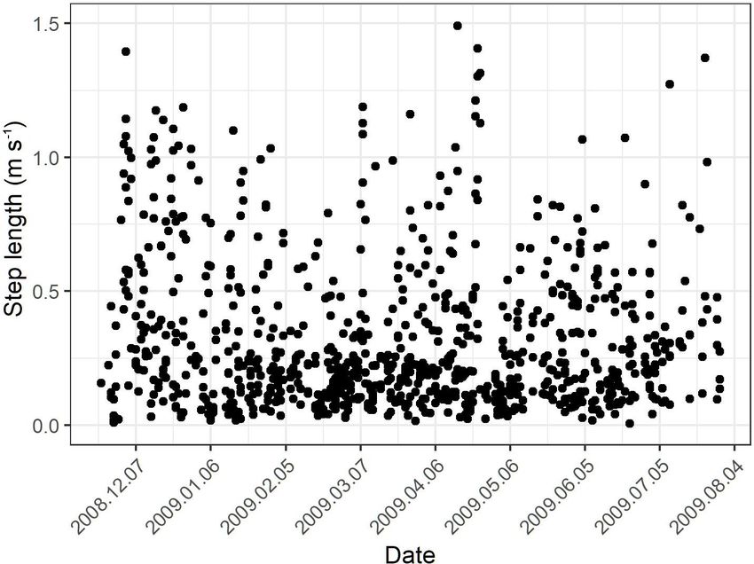
1938                                                 R. R. Togunov et al.: Opportunistic evaluation of modelled sea ice drift

can determine spatial distribution and configuration of dif-        ing moored Doppler-based velocity measures and other high-
ferent ice ages and thicknesses (Hutchings and Rigor, 2012;         resolution satellites (e.g., Advanced Very High Resolution
Mahoney et al., 2019). It also drives the rate of sea ice export,   Radiometer, AVHRR; or synthetic aperture radar, SAR), and
which affects ice extent throughout the Arctic (Rampal et           (2) in situ drifters, including buoys, ships, and manned sta-
al., 2009). Therefore, ice drift is often considered in models      tions (Lavergne et al., 2016). Other satellite-based estimates
of ice cover characteristics, overall sea ice mass throughout       are associated with their own estimation errors, and Doppler-
the Arctic, and global climate patterns (Hunke et al., 2010;        based validation represents only errors in the area in which
Kimura and Wakatsuchi, 2000; Kwok et al., 2013). In addi-           they are moored (Rozman et al., 2011). Some studies used in
tion to geographic and environmental studies, ice drift has         situ drifters (e.g., drifting research stations or buoys) as refer-
received increased attention in ecological research. Ice drift      ence data; however, they are consequently limited in spatial
influences the distribution and biomass of plankton (Hop and        extent (Hwang, 2013; Rozman et al., 2011; Tschudi et al.,
Pavlova, 2008; Kohlbach et al., 2017; Onodera et al., 2015;         2010). Since there are few sources of in situ sea ice drift data,
Thorpe et al., 2007), as well as polar bear (Ursus maritimus)       at least one study quantifying NSIDC drift accuracy used the
behaviour and energetics (Auger-Méthé et al., 2016a; Durner         same IABP data that are integrated into the NSIDC model for
et al., 2017; Mauritzen et al., 2003). In addition to its effects   validation, which may underestimate bias (e.g., Sumata et al.,
on geophysics and wildlife, ice drift is also important in de-      2014). Further, IABP buoys have historically used ARGOS
scribing transport of microplastics in the Arctic (Peeken et        location estimates, which have spatial errors up to tens of
al., 2018). Given its broad application, the accuracy of ice        kilometres and may be unsuitable for validation of drift dur-
drift data is critical when drawing geophysical and ecologi-        ing the periods/areas in which they were deployed (Hwang,
cal conclusions.                                                    2013).
   Several sources of ice drift data are available at variable         In this paper, we evaluate the bias and precision (here-
spatiotemporal resolutions (Sumata et al., 2014). Although          after collectively referred to as accuracy) of NSIDC drift
the data and models used vary between ice products, ice drift       data in Hudson Bay using an opportunistic and independent
estimates are generally estimated from combinations of buoy         source of sea ice drift validation data. We compared modelled
data, weather forecast models, and satellite measurements.          NSIDC drift to drifting GPS collars that were originally de-
These data sources vary in coverage, resolution, accuracy,          ployed on polar bears but dropped onto sea ice. There has
and sensitivity to environmental/meteorological conditions          been no study of the accuracy of any sea ice drift model in
and, therefore, result in products with variable sources of er-     Hudson Bay. In addition, the bay does not have any IABP
ror (Mahoney et al., 2019; Sumata et al., 2014). In this pa-        buoys, which drive the NSIDC model and its performance.
per, we sought to quantify these errors in a widely employed        Our objectives were to quantify drift accuracy within three
sea ice drift data product produced by the National Snow            domains: drift speed, drift direction, and the orthogonal (hor-
and Ice Data Center (NSIDC; Boulder, CO): Polar Pathfinder          izontal, u; and vertical, v) components of the drift vectors.
Daily 25 km EASE-Grid Sea Ice Motion Vectors (hereafter,            We also explored whether accuracy varied with the underly-
NSIDC drift; Tschudi et al., 2019, 2020). NSIDC drift esti-         ing drift speed, across months, or across years.
mates are produced by assimilating drift obtained from sev-
eral satellite-based sensors, buoys, and modelled wind fields,
providing among the most extensive, high-resolution, and            2   Methods
complete spatial coverage. In addition, the NSIDC drift prod-
uct has the longest temporal coverage of any sea ice drift          We fitted polar bears in western Hudson Bay, Canada, with
products extending from 1978 to the present (Tschudi et al.,        satellite-linked GPS collars (Telonics® , Mesa, Arizona) in
2020).                                                              August and September of 2004–2015 (Fig. 1). Procedures
   Although research has examined the accuracy of older             for animal capture and handling are described by Stirling
versions of NSIDC drift (e.g., Ruslan, 2018; Schwegmann             et al. (1989) and were approved annually by the University
et al., 2011; Sumata et al., 2014, 2015b), the latest ma-           of Alberta Animal Care and Use Committee for Biosciences
jor release (version 4.0) has yet to be externally evaluated.       and by the Environment and Climate Change Canada West-
The NSIDC drift model integrates the movement of buoys              ern and Northern Region Animal Care Committee. Protocols
from the International Arctic Buoy Program (IABP; http:             were in accordance with the Canadian Council on Animal
//iabp.apl.washington.edu/, last access: 10 June 2020), and         Care. Collars were programmed to obtain GPS fixes every
the buoys are the highest weighted input source driving the         4 h. The locations obtained have a high accuracy, with er-
NSIDC model (Sumata et al., 2015a). Regions without such            rors < 31 m (D’Eon et al., 2002). Although deployed with
in situ measurements are more susceptible to bias (Mahoney          the purpose of studying polar bear behaviour and space use,
et al., 2019; Sumata et al., 2015a; Tschudi et al., 2020) and       some collars may slip off the bears, they may release early
are therefore particularly important to evaluate.                   due to premature failure of the release mechanism, or the
   There are two types of data that can be used to cross val-       bear may die while the collars continue to transmit locations.
idate ice drift: (1) other telemetry-based estimators includ-       In these instances, the observed displacement of the collars

The Cryosphere, 14, 1937–1950, 2020                                                     https://doi.org/10.5194/tc-14-1937-2020
R. R. Togunov et al.: Opportunistic evaluation of modelled sea ice drift 1939
tance weight (inverse distance power set to three and maxi-
mum distance of 50 km) to match the fix location.
The summary statistics chosen to quantify drift accuracy
can lead to incomplete or spurious conclusions (Volkov et
al., 2017). For example, root mean square and standard er-
rors convey the magnitude of the error but not the direction.
Correlation coefficients between model and reference data
describe model precision but not accuracy. Some studies in-
vestigated the accuracy of the orthogonal components of drift
(i.e., u and v) individually; however, this does not convey the
accuracy in speed and direction, which are emergent proper-
ties of both components. For example, if the biases of the or-
thogonal components are equal and scale proportionally, then
direction estimates remain accurate. Conversely, if the biases
are negatively correlated, they may partially cancel and result
in speed estimates more accurate than appear when examin-
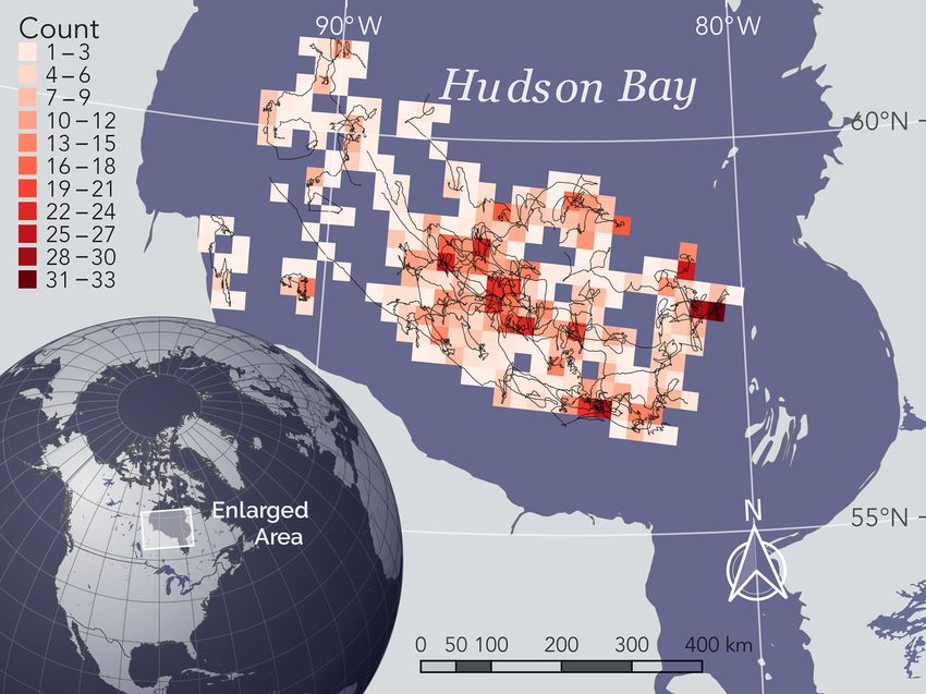
Figure 1. Hudson Bay study area (enlarged), tracks of dropped col- ing the drift components independently. Thus, in addition to
lars (black lines), and count of drift vectors (shaded cells, projected the orthogonal u and v components of drift, we also quanti-
in 25 km EASE-Grid North, EPSG: 3408). World borders dataset fied the accuracy of drift speed and direction.
obtained from Sandvik (2009). We tested the following five key questions. (1) Are the
estimated model speeds significantly different from the col-
lar speeds? (2) Is the relative speed accuracy dependant on
represents the motion of sea ice. We identified drifting col- the underlying drift speed being estimated? (3) Are the esti-
lars either through activity sensors in the collars or by man- mated model directions significantly different from the col-
ually comparing the observed collar displacement with sea lar directions? (4) Is the direction accuracy dependant on
ice satellite imagery (Appendix A). To verify that manually the underlying drift speed? And (5) do the relationships
identified drifting collars were passively drifting and not on between the model u (v) and collar u (v) components di-
active bears, we compared accuracy metrics for speed, di- verge significantly from each other? Because the data are
rection, and u and v (relative to the NSIDC drift projection, spatiotemporally autocorrelated, with subsequent days hav-
EPSG: 3408) among activity sensor collars, manually iden- ing similar drift speeds and different collars sampling dif-
tified passive collars, and collars on active bears. Detailed ferent regions of Hudson Bay, we could not use a simple
methods and results of this comparison are presented in the paired t test for the absolute speed bias (1). Instead, we used
Appendix B. an intercept-only generalized linear mixed model (GLMM;
We used the motion of the identified drifting collars (fol- with a Gaussian error distribution) with absolute speed bias
lowing date of inactivity/drop off; hereafter simply collars) (SpeedNSIDC − Speedcollar ) as the response, wherein a signif-
to quantify the accuracy and precision of NSIDC drift data. icant intercept represents a significant difference between the
The NSIDC product provides daily estimates of sea ice drift model and the collar speeds. To account for repeat sampling
derived from buoy data; National Centers for Environmen- from different collars representing different regions, collar
tal Prediction and National Center for Atmospheric Research identity was used as a random effect. To account for tem-
reanalysis wind vectors; and several satellite sensors includ- poral autocorrelation, we fit the model with a first-order au-
ing AVHRR, the Advanced Microwave Scanning Radiometer toregressive error process (AR1). For speed-dependant ac-
for the Earth Observing System (AMSR-E), Scanning Mul- curacy of model speed (2), we defined relative speed accu-
tichannel Microwave Radiometer (SMMR), and the Special racy as the quotient of NSIDC drift speed over collar speed,
Sensor Microwave Imager/Sounder (SSMI/S; Tschudi et al., SpeedNSIDC
Speedcollar , with values > 1 representing overestimation and
2019, 2020). To match the NSIDC product, collar locations values < 1 representing underestimation. This relative speed
were projected into the 25 km EASE-Grid North (EPSG: accuracy was modelled as a function of log(Speedcollar ) us-
3408) projection used by NSIDC. NSIDC represents drift ing GLMMs with gamma error distribution and a log-link
as movement between 12:00 UTC of subsequent days. To function. We log transformed Speedcollar because it is zero
match the NSIDC temporal resolution, we subsampled the bound and the relative difference in speed (and thus its rel-
collar locations to a 24 h resolution by retaining locations ative effect on model accuracy) decays exponentially with
from 13:00 UTC, the closest collar location to 12:00 UTC. increasing values. We used the same random effect and AR1
Next, we calculated drift vectors/components (i.e., speed, di- structure as in (1). We assessed the accuracy of model di-
rection, u, and v) and then removed any vectors from loca- rection, DirectionNSIDC −Directioncollar , (3) using a Watson–
tions > 24 h apart. Next, we interpolated the NSIDC drift to Williams test for homogeneity of means for circular data. Al-
the first location of each collar drift vector using inverse dis-
https://doi.org/10.5194/tc-14-1937-2020 The Cryosphere, 14, 1937–1950, 2020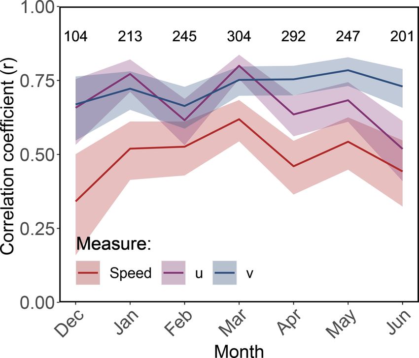
1940 R. R. Togunov et al.: Opportunistic evaluation of modelled sea ice drift
Figure 2. Autocorrelation function (ACF) for NSIDC linearized Figure 3. Interannual variation in correlation coefficients (r) be-
direction accuracy, tan(|DirectionNSIDC − Directioncollar |/2). Blue tween NSIDC drift and collar drift speed (red line), u component
lines correspond to the 95 % confidence interval (CI) limits that rep- (purple line), and v component (blue line). Shaded areas represent
resent significant autocorrelation. the 95 % CI of the correlation coefficient. Numbers at the top repre-
sent the number of drift vectors compared in each year. Year 2013
is excluded due to insufficient data (n = 4).
though this test does not incorporate autocorrelation, the ab-
solute direction accuracy did not exhibit temporal autocorre-
lation (Fig. 2). For the speed-specific direction accuracy (4), 3 Results
we defined relative direction accuracy
as the linearized abso-
|DirectionNSIDC − Directioncollar |
lute difference in direction, tan 2 , We identified 20 drifting collars with locations from
where 0 represents model unanimity and departure from 0 December–July of 2005–2015 (Figs. 1 and 3), with a mean of
represents increasing error. This relative direction accuracy 520 ± 358 GPS fixes per collar (total = 10 409). The largest
was modelled as a function of log(Speedcollar ) using the same number of identified collars in 1 year was in 2009 (n = 6).
GLMM procedures used for testing speed-specific relative The motion for these six collars is depicted in the Video
speed accuracy (2). Any differences in speed or direction be- supplement (https://doi.org/10.5446/45186, Togunov et al.,
tween the NSIDC and collar drift ultimately emerge from 2020), which depicts the large degree of concurrence of drift
the estimated u and v components of sea ice drift. We as- vectors across large spatial extent. After subsampling to a
sessed the relationship between the orthogonal components daily resolution, we analyzed 1677 collar drift vectors. The
of NSIDC and collar drift (5) using GLMM (with a Gaussian number of drift vectors ranged from 71 vectors in July to 304
error distribution), with model u (v) modelled as functions vectors in March (mean = 210 ± 83 vectors; Fig. 4).
of collar u (v), and the same random effect and AR1 struc-
ture as in (1), (2), and (4). All GLMMs were fit using pe- 3.1 Accuracy of NSIDC drift speed
nalized quasi-likelihood (GLMMPQL ; Breslow and Clayton,
1993) using the glmmPQL function of the MASS package Mean NSIDC drift speed was 5.8 ± 4.5 km d−1 while
(Venables and Ripley, 2002). Using GLMMPQL enabled us mean collar speed was 8.4 ± 7.1 km d−1 ; the difference in
to meet all our model criteria: non-linear models with ran- speed SpeedNSIDC − Speedcollar was statistically significant
dom effects and an autoregressive structure. As a broad met- (GLMMPQL : intercept ±95 % confidence interval (CI) =
ric of goodness of fit, we used the GLMMPQL R 2 metric de- −3.0 ± 1.2 km d−1 , degrees of freedom (df) = 1657, t value
veloped by Jaeger et al. (2017) using the r2beta function in = −4.8, p value < 0.0001; Fig. 5). NSIDC drift speeds
the r2glmm package. All data processing and analyses were were slower than collar drift speeds in 63.1 % of the vec-
conducted in R version 3.6.1 (R Core Team, 2019). tors, and only 10.4 % of NSIDC drift speeds were within
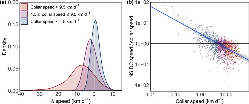
±10 % of collar drift speeds (Fig. 5a). The discrepancy
in drift speed was more pronounced at higher collar drift
speeds, with a significant relationship between the quotient
Speed
( SpeedNSIDC ) and collar speed (GLMMPQL : slope = −0.67, df
collar
= 1656, t valueslope = −38.80, p valueslope < 0.0001, R 2 =
0.53; Fig. 5b). Collar drift speeds < 4.5 km d−1 were over-
The Cryosphere, 14, 1937–1950, 2020 https://doi.org/10.5194/tc-14-1937-2020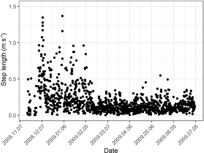
R. R. Togunov et al.: Opportunistic evaluation of modelled sea ice drift 1941
37.58, p valueslope < 0.0001, R 2 = 0.46; Fig. 8) and the v
component (GLMMPQL : slope ±95 % CI = 0.40 ± 0.02, df
= 1656, t valueslope = 37.54, p valueslope < 0.0001, R 2 =
0.52; Fig. 8). Although the components of NSIDC drift and
collar drift were significantly correlated, the slopes of the re-
gression were significantly underestimated (indicated by the
slope estimate and 95 % CI being < 1).
4 Discussion
Using drifting collars as reference data for validation, we
identified biases in the estimated speed and direction of the
NSIDC sea ice drift model. NSIDC drift speeds tended to be
underestimated, although drift direction was relatively accu-
rate. This is due to the underestimation of u and v compo-
nents, which showed a similar magnitude in their bias. The
Figure 4. Intra-annual variation in correlation coefficients (r) be- biases in speed and direction were related to the underlying
tween NSIDC drift and collar drift speed (red line), u component drift speed as measured by the collars. NSIDC drift speeds
(purple line), and v component (blue line). Shaded areas represent tended to overestimate slow collar drift (< 4.5 km h−1 ) and
the 95 % CI of the correlation coefficient. Numbers at the top rep- underestimate high collar drift (> 4.5 km h−1 ). This pattern
resent the number of drift vectors compared in each month. July is is likely an effect of estimating a zero-bound variable and
excluded due to insufficient data (n = 71). is consistent with other satellite-based sea ice drift products
(Johansson and Berg, 2016; Mahoney et al., 2019; Rozman
et al., 2011; Sumata et al., 2014). As drift speeds approach
estimated by a median of 42 %, speeds between 4.5 and 0 km d−1 , the probability of overestimation approaches 1,
9.0 km d−1 were underestimated by a median of 26 %, and and as drift speeds increase, the range of values that are be-
speeds > 9.0 km d−1 were underestimated by a median of low the drift speed (i.e., underestimates) increases. Although
51 % (Fig. 5). There was intra-annual and inter-annual vari- the bias is mathematically inevitable to some degree, the
ation (based on 95 % CIs) in the correlation of NSIDC drift magnitude of the bias is not fixed, and our results show that
speeds and collar drift speeds; however, there was no appar- the error can be high, with drift speeds underestimated by
ent pattern (Figs. 3 and 4). a median of 22.9 % (1.4 km d−1 ). This is similar to the drift
bias observed by Durner et al. (2017) in the Beaufort and
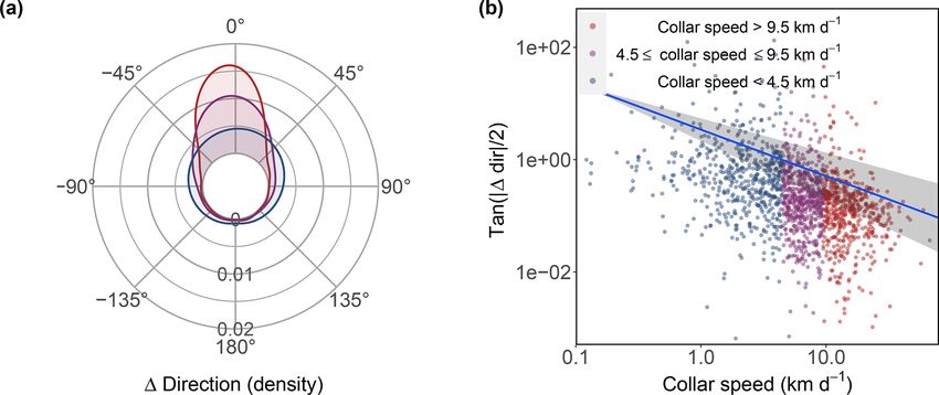
3.2 Accuracy of NSIDC drift direction
Chukchi seas, wherein mean daily model speed was under-
NSIDC drift directions were on average 2.6◦ ± 53.9◦ left estimated by a mean of 28.0 % (2.25 km d−1 ). These biases
relative to the collar drift direction, although the mean dif- are small relative to the 25 km resolution of the satellite in-
ference was not significantly different from 0◦ (Watson– put data; however, in some analyses, the bias would com-
Williams test: df1 = 1, df2 = 1676, F value = 0.003, p value pound over time. For example, cumulative/total daily drift
= 0.95; Figs. 6 and 7). Most (71.3 %) of the NSIDC drift calculated for 7 months (corresponding to the months in
directions were within ±22.5◦ of the collar drift directions which we obtained drift data) would be underestimated by
(Fig. 7). NSIDC drift direction tended to be more accurate > 295 km. Drift direction accuracy increased at higher collar
at higher collar drift speeds, with a significant relationship drift speeds. This is probably because magnitude and uni-
between relative direction accuracy and collar drift speeds formity of sea ice displacement increase with drift speed,
(GLMMPQL : slope = −0.83, df = 1656, t valueslope = and this is more likely to be detected by NSIDC’s feature-
−7.52, p valueslope < 0.0001, R 2 = 0.03; Fig. 7). matching algorithm (based on maximum cross correlation;
Tschudi et al., 2019).
3.3 Accuracy of orthogonal NSIDC drift components Our estimates of drift speed bias are greater than estimated
in studies of NSIDC and other drift products (Durner et al.,
Mean collar drift u component was −0.9 ± 7.7 km d−1 2017; Hwang, 2013; Johansson and Berg, 2016; Lavergne,
compared to −0.7 ± 4.3 km d−1 for NSIDC drift u drift. 2016; Schwegmann et al., 2011; Sumata et al., 2014). How-
Mean collar drift v component was −1.1 ± 7.7 km d−1 com- ever, the Hudson Bay system is different from areas where
pared to −0.8 ± 4.5 km d−1 for NSIDC drift v compo- drift accuracy has been studied. First, Hudson Bay has a
nent drift. NSIDC and collar drift components were sig- smaller area-to-shoreline ratio due to its smaller size com-
nificantly related in both the u component (GLMMPQL : pared to the rest of the Arctic Ocean (excluding the Canadian
slope ±95 % CI = 0.38 ± 0.02, df = 1656, t valueslope = Arctic Archipelago), which confounds satellite and wind-
https://doi.org/10.5194/tc-14-1937-2020 The Cryosphere, 14, 1937–1950, 2020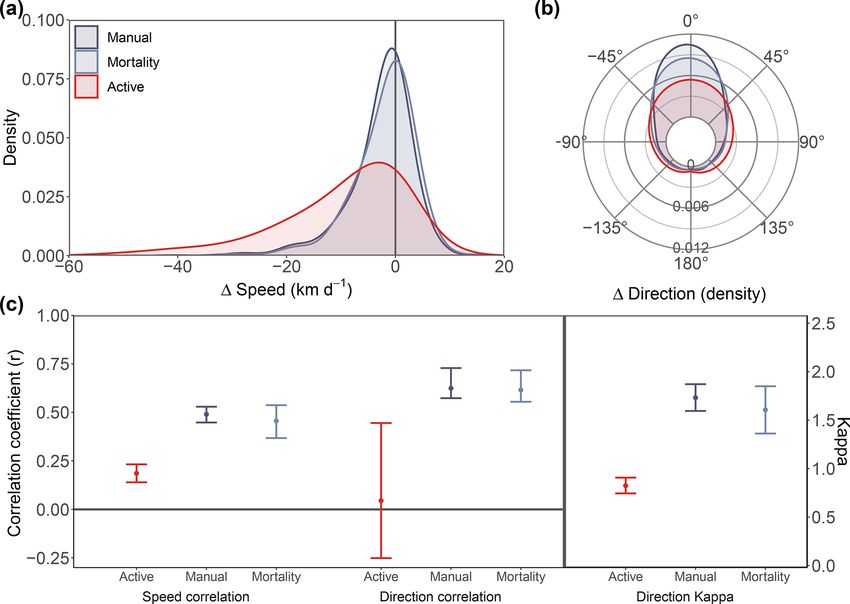
1942                                                    R. R. Togunov et al.: Opportunistic evaluation of modelled sea ice drift

Figure 5. Accuracy of NSIDC drift speed represented by (a) a histogram and density plot of the absolute accuracy (SpeedNSIDC −Speedcollar )
and (b) GLMMPQL of relative accuracy (SpeedNSIDC /Speedcollar ) as a function log-transformed collar speed (presented on log–log scale;
the blue line is the GLMPQL prediction of the mean with the shaded 95 % CI). In both (a) and (b), data points are separated into three groups
(red, purple, and blue) based on collar speed to convey speed-specific variability in accuracy. Black lines represent 1 : 1 unanimity between
NSIDC and collar drift speeds.

Figure 6. Accuracy of NSIDC drift direction represented by (a) a circular histogram and density plot of the absolute accuracy
(DirectionNSIDC − Directioncollar ) and (b) GLMMPQL of relative accuracy (tan(|DirectionNSIDC − Directioncollar |/2)) as a function of log-
transformed collar speed (presented on a log–log scale, with a zero value representing 1 : 1 unanimity); the blue line in (b) represents the
GLMMPQL prediction of the mean with the shaded area representing the 95 % CI. Data points are separated into three groups (red, purple,
and blue) based on collar speed to convey speed-specific variability in accuracy.

based drift estimation (Thorndike and Colony, 1982; Tschudi              tion of wind relative to the shoreline. Near the coast, inter-
et al., 2020). Satellite-based tracking relies on a feature-             nal ice stress/forces can exceed those of wind and currents,
matching algorithm and cannot resolve velocities near the                with the effects extending up to 400 km (Fissel and Tang,
shore (Heil et al., 2001; Meier et al., 2000; Tschudi et al.,            1991; Overland and Pease, 1988; Rabinovich et al., 2007;
2020). While currently NCEP wind is weighted half as much                Thorndike and Colony, 1982). More complex regression-
as buoy or satellite data, Tschudi et al. (2020) noted that              based models that account for proximity and orientation of
wind-based estimates are comparable to satellite estimates               shorelines have been shown to improve wind-based drift esti-
and may need to be given a higher weight. Although giv-                  mates (Rabinovich et al., 2007). Second, the bay is a seasonal
ing wind estimate higher weight may improve drift estimates              system, completely melting in summer and reaching nearly
in Hudson Bay, it may still result in speed underestimation.             100 % cover in winter (Danielson, 1971; Saucier et al., 2004;
Wind-based drift estimates assume a 20◦ relationship with                Stewart and Barber, 2010). Consequently, sea ice in Hudson
direction and a 1 % relationship with speed, although this               Bay lacks multi-year ice, and the ice is younger and generally
speed relationship may actually be higher (up to 3 %; Bai et             thinner, with extensive periods of low concentration, factors
al., 2015; Rabinovich et al., 2007). The effect of wind on drift         which both decrease accuracy of modelled ice drift (Durner
also varies depending on proximity to shore and the orienta-             et al., 2017; Mahoney et al., 2019; Sumata et al., 2014). At

The Cryosphere, 14, 1937–1950, 2020                                                           https://doi.org/10.5194/tc-14-1937-2020
R. R. Togunov et al.: Opportunistic evaluation of modelled sea ice drift                                                          1943

                                                                       given to the wind input data, lack of buoy data, and projection
                                                                       biases.
                                                                          A common limitation of these types of studies is
                                                                       the reliance on interpolation. Bilinear, or inverse-distance-
                                                                       weighted, interpolation yields estimates that tend towards the
                                                                       mean and precludes obtaining outermost estimates (Schweg-
                                                                       mann et al., 2011). In addition, interpolation within skewed
                                                                       distributions is likely to yield spurious estimates. For exam-
                                                                       ple, in right-skewed datasets (e.g., zero-bound drift speed),
                                                                       outliers are more likely greater than the mean, and inverse-
                                                                       distance averaging is more likely to be an overestimate. Nev-
                                                                       ertheless, there is no reason to believe these biases would be
                                                                       greater than those of other sea ice drift validation studies that
                                                                       used linear interpolation to match satellite with in situ-based
                                                                       estimates (Lavergne, 2016; Schwegmann et al., 2011).
                                                                          The drift biases we report are limited by availability of
                                                                       telemetry collar data, and we cannot definitively extrapo-
                                                                       late our accuracy estimates beyond this spatiotemporal ex-
Figure 7. Difference between collar drift and NSIDC drift for the      tent. Nevertheless, many of these biases have been reported
u (x axis) and v (y axis) components. Curves represent density of      in research of NSIDC and other satellite-based sea ice drift
differences, and the red dot represents the mean difference of u and   estimates (Heil et al., 2001; Karlsson, 2016; Lavergne, 2016;
v components.
                                                                       Linow et al., 2015; Rozman et al., 2011; Schwegmann et al.,
                                                                       2011; Sumata et al., 2014, 2015b, 2015a; Szanyi et al., 2016).
                                                                       Areas with similar characteristics to Hudson Bay may show
                                                                       similar biases in the estimated speed and direction of drift.
low ice concentrations, satellites sensors are more likely not         This includes other seasonal systems (e.g., Baffin Bay) and
to detect sea ice (Castro de la Guardia et al., 2017; Tivy et al.,     those with slower drift (e.g., Kara and Laptev seas) or with-
2011). The formation of new sea ice during freeze-up and the           out IABP buoys (see IABP, 2020, and Rampal et al., 2009,
melt ponds that form during break-up both confound estima-             for coverage). Further, we observed the relative degree of
tion of drift (Meier et al., 2000; Tschudi et al., 2020; Willmes       bias increases with speed. If such scaling in bias exists in
et al., 2009). Third, there are no IABP buoys in Hudson Bay            other areas, then the magnitude of underestimation may be
to contribute data to the NSIDC drift model, another factor            greater in areas with faster speeds (e.g., Chukchi Sea).
associated with poorer model performance (Mahoney et al.,                 Assuming the overall NSIDC drift accuracy is consistent
2019; Tschudi et al., 2020). Earlier versions of NSIDC drift           over time, these data are likely well suited for addressing
products (see Tschudi et al., 2016) effectively limited the            questions where the relative speed or direction are sufficient,
influence of buoys to ∼ 350 km, which introduced artefacts             for example longitudinal analyses such as climate-induced
around buoy locations (Szanyi et al., 2016). Changes to the            changes in drift speed (e.g., Kwok et al., 2013; Klappstein
algorithm in version 4 of NSIDC drift eliminated the artefacts         et al., 2020). Still, a large error may obscure underlying
and increased accuracy within the Arctic Ocean (Tschudi et             trends. We suggest cautious application of the NSIDC drift
al., 2020); however, these changes would not have improved             data where the absolute speed or direction is critical – for ex-
drift estimates in regions without buoy data, including Hud-           ample, calculation of animal energetics (e.g., Durner et al.,
son Bay. Last, the EASE-Grid projection is polar azimuthal             2017; Klappstein et al., 2020), home ranges (e.g., Auger-
and induces meridional compression and zonal stretching,               Méthé et al., 2016a), voluntary movement (e.g., Togunov et
which further biases drift estimation. The effect of this distor-      al., 2017, 2018), and predicting/retrodicting distribution of
tion is that north–south (east–west) drift is more likely to be        drifting matter (Kohlbach et al., 2017; Peeken et al., 2018;
underestimated (overestimated), and direction estimates will           Thorpe et al., 2007; Tschudi et al., 2010). The degree of er-
be biased toward the east–west axis. This bias is amplified as         ror/bias that is permissible is research specific. Generally, to
you approach the equatorial limits of the dataset and is par-          be able to correctly account for measurement error, it has to
ticularly important if groundspeed is required. Hudson Bay is          be smaller than the natural stochasticity of the system be-
the furthest body of water from the poles where NSIDC drift            ing studied (Auger-Méthé et al., 2016b). Particular attention
is estimated and would therefore experience the greatest bias          to error/bias should be given in regions without IABP buoy
due to projection. In summary, our observed speed underes-             data or where bias is unquantified.
timation may be explained by the challenging topography of
Hudson Bay for satellite and wind-based drift estimates, un-
derestimation of wind’s impact on ice motion, small weight

https://doi.org/10.5194/tc-14-1937-2020                                                      The Cryosphere, 14, 1937–1950, 2020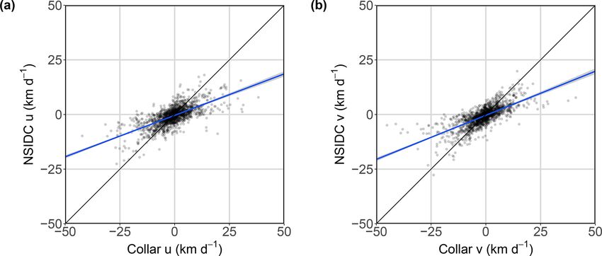
1944                                                    R. R. Togunov et al.: Opportunistic evaluation of modelled sea ice drift

Figure 8. GLMMPQL (family: Gaussian) regression of the u (a) and v (b) components of NSIDC drift vector versus collar drift. Black lines
represent a 1 : 1 relationship between NSIDC and collar drift components; the blue lines represent the lines of best fit with the shaded areas
representing the 95 % CI of the mean.

5   Conclusions                                                          Hudson Bay, where a lack of Arctic buoys makes this type
                                                                         of study difficult. Ultimately, these findings (in combination
This study provides the first error estimates of any sea ice             with our public dataset and that of other drifting tag data;
drift model in Hudson Bay. Using passively drifting teleme-              Durner et al., 2017; Øigård et al., 2010; Vacquie-Garcia et
try collars, we quantified the accuracy and precision of Po-             al., 2017) can be a good resource for quantifying and validat-
lar Pathfinder Daily 25 km EASE-Grid Sea Ice Motion Vec-                 ing the accuracy of other and/or future ice drift products.
tors, Version 4. Both u and v components of NSIDC drift
along with the resultant speed tended to systematically un-
derestimate true drift speed, a pattern exacerbated at higher
speeds. The direction showed no systematic bias; however,
directional precision decreased at lower speeds. We sug-
gest that any research requiring absolute values for drift
speed/direction should account for error/bias of drift in the
study design and/or test the sensitivity of the results to these
biases (Cressie et al., 2009).
   Although our collar GPS data were collected with the in-
tent of studying polar bear ecology, we believe it and other
forms of animal-borne telemetry can be of great utility in ad-
vancing environmental modelling. For example, polar bear
telemetry has been used to validate sea ice drift in the Beau-
fort and Chukchi seas (Durner et al., 2017; Tschudi et al.,
2010) and to assess accuracy of sea ice concentration data
(Castro de la Guardia et al., 2017), and seabird tracking
has been used to estimate ocean currents and wind veloci-
ties (Goto et al., 2017; Yoda et al., 2014; Yonehara et al.,
2016). In addition to being useful for model validation, these
types of data can be incorporated into environmental mod-
els as additional data streams, providing insight into areas
that are more difficult to measure (Harcourt et al., 2019;
Miyazawa et al., 2015). To help improve modelled drift
data, we have made the position data of our drifting collars
public https://doi.org/10.7939/dvn/kuiz7g (Derocher, 2020).
The data can also be used to identify error/bias associated
with different locations, periods, or environmental conditions
(e.g., ice thickness, ice concentration, and cloud cover) in
which models can be improved (e.g., Miyazawa et al., 2015).
Our study provides evidence of modelled ice drift bias in

The Cryosphere, 14, 1937–1950, 2020                                                            https://doi.org/10.5194/tc-14-1937-2020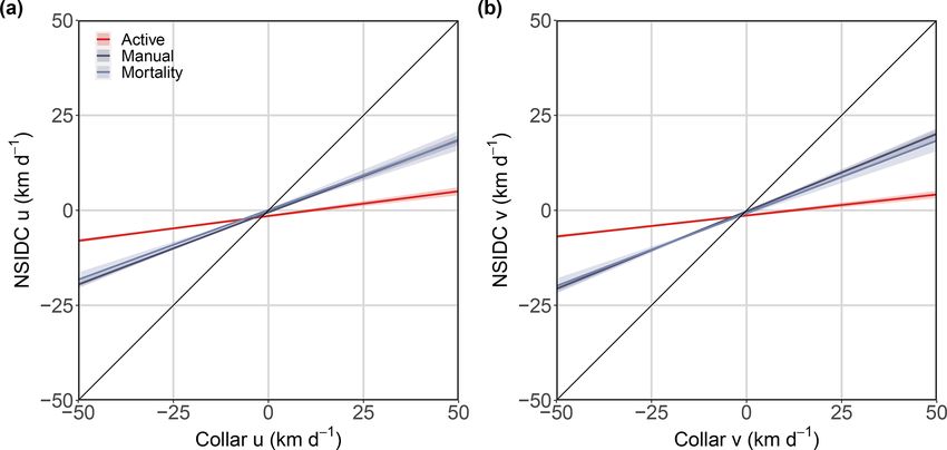
R. R. Togunov et al.: Opportunistic evaluation of modelled sea ice drift                                                        1945

Appendix A: Drifting collar identification

Collars deployed since 2011 were equipped with activity sen-
sors that are triggered following an extended period of inac-
tivity. These collars were considered passively drifting if the
activity sensor turned on and stayed until the end of trans-
missions. Collars deployed before 2011 had to be identified
manually in two stages.
   First, GPS location data were annotated with sea ice mo-
tion vectors from NSIDC’s Polar Pathfinder Daily 25 km
EASE-Grid Sea Ice Motion Vectors, Version 3 (http://nsidc.
org/data/nsidc-0116, last access: 10 June 2020). Daily drift
estimates were spatiotemporally interpolated to match the lo-
cation and time of GPS fixes – it was assumed that the ice
motion data reflected average drift at noon of each day. For
all 4 h GPS fixes, voluntary bear movement was estimated
by subtracting the component of ice drift from the GPS dis-         Figure A1. Example of estimated voluntary movement (step length
placement. This estimate of voluntary movement was plot-            in m s−1 ) over time of a collar that is on a living bear.
ted against time for each collar. Collars were suspected to be
drifting if there was a sudden and sustained drop in move-
ment speed (e.g., Fig. A1 versus Fig. A2). To confirm that          of the collar location (hereafter, first-day ice location), and
the collars are indeed drifting, the displacement of these sus-     another point was marked where that same ice floe was on
pect collars had to be confirmed to reflect the actual sea ice      the following day (hereafter, second-day ice location). Sixth,
drift.                                                              both marks were selected using selection tool in AnnotatePro
   Actual sea ice drift was derived from NASA’s Earth Ob-           and moved such that the first-day ice location overlapped the
serving System Data and Information System (EOSDIS)                 first-day collar location. The second-day ice location repre-
satellite imagery (https://earthdata.nasa.gov/about, last ac-       sented where the collar would be located on the following
cess: 10 June 2020). First, the projection and scale of EOS-        day had the bear not moved. If the collar location was on an
DIS and collar locations had to be matched. The EOSDIS              identified ice floe, only that floe was tracked. If the collar lo-
Worldview web interface (https://worldview.earthdata.nasa.          cation was not on an identified floe, up to five additional floes
gov/, last access: 10 June 2020) projection was set to “Arc-        around the collar location were identified and marked to at-
tic” (WGS 84/NSIDC Sea Ice Polar Stereographic North pro-           tain an approximation of drift at the collar location. Seventh,
jection; EPSG: 3413), rotated −69◦ , and maximally zoomed           the distance between second-day ice location and the second-
in. Collar locations were plotted in QGIS version 2.16.3;           day collar location was calculated using the “measure line”
the projection was matched to EOSDIS (EPSG: 3413) and               tool in QGIS. If several ice floes were marked and tracked,
scaled in QGIS to 1 : 480 000 (though the realized scale was        then the distance was measured from the second-day collar
∼ 1 : 1 330 000 on the 13.3 in. computer at a 2560×1600 res-        location to the approximate centre of all the second-day ice
olution).                                                           floe locations. At the operating scale being used, sea ice drift
   Next, sea ice drift was estimated at a subset of loca-           was relatively uniform, and there was very high consistency
tions for each suspected drifting collar using the follow-          in drift among ice floes.
ing procedure. First, the view in QGIS was centred on                  Collars were assumed to be passively drifting collars if
GPS locations of a probably drifting collar where ice drift         the mean of at least four consecutive distance estimates
would be approximated, and the view in EOSDIS World-                (hereafter, distance estimate) was < 2 km (hereafter, distance
view was matched. Second, we identified periods where the           threshold). At the maximum resolution permitted in EOS-
satellite imagery was relatively unobscured by clouds for           DIS, the 2 km distance threshold corresponded to ∼ 1.5 mm
at least 2 d and visually tracking ice floes would be possi-        on screen. If the distance estimate was greater than the dis-
ble. Third, a collar location representing the first location       tance threshold, the collar was assumed to be on a live bear
of a displacement vector (hereafter, first-day collar loca-         and not a drifting collar.
tion) was marked using the screen annotation software Anno-            The EOSDIS imagery used was taken during daylight
tatePro (https://web.archive.org/web/20190701171427/http:           hours, so sea ice drift was estimated (as much as possible)
//www.annotatepro.com:80/, last access: 31 July 2018).              for collar locations at 17:00 and 21:00 UTC, generally corre-
Fourth, we identified unique sea ice features that could be         sponding to midday in Hudson Bay. For each suspect drift-
tracked over both days. Unique ice features were mainly dis-        ing collar, sea ice drift was first estimated for the last days
tinctive edges and corners of ice floes and fractures. Fifth, us-   of collar locations; if the distance estimate was greater than
ing AnnotatePro, we marked where an ice floe was on the day         the distance threshold (i.e., indicating a live bear), all prior

https://doi.org/10.5194/tc-14-1937-2020                                                   The Cryosphere, 14, 1937–1950, 2020

1946                                                 R. R. Togunov et al.: Opportunistic evaluation of modelled sea ice drift

                                                                    Appendix B: Drifting collar validation

                                                                    To lend additional support that manually identified collars
                                                                    were indeed not on active bears, we compared metrics of
                                                                    speed, direction, and u and v component accuracy calculated
                                                                    for manually identified collars, activity-sensor-identified col-
                                                                    lars, and active collars. First, we subset the active collars to a
                                                                    24 h resolution by filtering only fixes obtained at 13:00 UTC.
                                                                    Second, we calculated the displacement vectors (speed, di-
                                                                    rection, and u and v components; calculated in the EASE-
                                                                    Grid North projection, EPSG: 3408) between successive
                                                                    days, and then we filtered any vectors representing displace-
                                                                    ment over > 24 h. Third, we subset the active collar vector
                                                                    data to the same number of locations as the drifting col-
                                                                    lars (n = 1677) and only in the years (2005, 2008–2010, and
                                                                    2013–2015) and months (December–June). These data were
Figure A2. Example of estimated voluntary movement (step length     then compared to drifting collars identified manually and us-
in m s−1 ) over time of a suspect passive collar.                   ing the activity sensor.
                                                                       The metrics of comparison were speed accuracy
                                                                    (SpeedNSIDC − Speedcollar ; Fig. B1a) and direction ac-
locations must also have been on a live bear. If the distance       curacy (DirectionNSIDC − Directioncollar ; Fig. B1b). We also
estimates were less than the distance threshold the collar was      tested the correlation in speed, direction, u component, and
assumed to be drifting, then drift was estimated iteratively        v component between NSIDC drift estimates and collar
∼ 30 d into the past until the distance estimate indicated a        displacement vectors (Figs. B1c and B2). For speed, we
live bear. Next, from the last date assumed to be drifting, sea     calculated the Pearson correlation coefficient (Fig. B1c).
ice drift was estimated iteratively ∼ 7 d into the past until the   For direction, we calculated the circular Pearson correlation
mean distance estimate indicated a live bear. Finally, from the     coefficient (±95 % CI) using the “cor.circular” function in
last drifting collar date, we examined prior days sequentially      the “circular” package in R. We used bootstrapping with
until the distance estimate indicated a live bear. The follow-      1000 replicates to calculate the 95 % CI for this circular
ing day was determined to be the date when the collar either        correlation (Fig. B1c). As an additional metric of directional
dropped off the bear or the bear died.                              accuracy, we estimated the concentration parameter (kappa
   For certain days, ice drift estimation was either very poor      ±95 % CI) on the difference between NSIDC drift and collar
or not possible. Confounding factors included heavy cloud           displacement vectors (Fig. B1c). Last, we fit a glmmPQL
cover, blurry satellite imagery, small floes that were indis-       function (family: Gaussian) with the NSIDC drift u and v
tinguishable and not trackable (particularly common during          components as functions of u and v components of active,
freeze-up and break-up), consolidated ice with no trackable         manually identified, and activity-sensor-identified collars
features, or days with extreme fracturing of ice floes beyond       (Fig. B1).
recognition. For these periods, certain modifications to the           There were no significant differences between manually
described protocols were permitted. For example, if cloud-          identified drifting collars (n = 13) and collars identified us-
free days were separated by up to two clouded days and sea          ing activity sensor (n = 7) in accuracy metrics of speed, di-
ice drift could be estimated across that period, this was per-      rectional, or u and v components. However, both manually
mitted. If many of the drift estimates were poor, researcher        and activity-sensor-identified collars were consistently sig-
discretion was permitted to increase the drifting collar thresh-    nificantly different from collars on active bears with regard
old from 2 km. During periods with extensively poor ice drift       to the same accuracy metrics (Figs. B1 and B2). All results
estimation, if four sequential drift estimates spanned beyond       exhibit a significantly weaker relationship between NSIDC
a week, it was permitted to average fewer than four estimates.      drift and displacement of active collars compared to either
                                                                    passively drifting collars.
                                                                       The motion for six manually identified collars is depicted
                                                                    in the Video supplement (https://doi.org/10.5446/45186, To-
                                                                    gunov et al., 2020). This video depicts the large degree of
                                                                    concurrence of drift vectors across a large spatial extent and
                                                                    further supports that the manually identified collars are in
                                                                    fact passively drifting.

The Cryosphere, 14, 1937–1950, 2020                                                     https://doi.org/10.5194/tc-14-1937-2020
R. R. Togunov et al.: Opportunistic evaluation of modelled sea ice drift 1947 Figure B1. Comparison of speed and direction metrics of collars believed to be on active bears (red), manually identified drifting col- lars (dark blue), and activity-sensor-identified drifting collars (light blue). Metrics presented are density plot of the difference in speed, (SpeedNSIDC − Speedcollar ; a), density plot of difference in direction (DirectionNSIDC − Directioncollar ; b), Pearson’s correlation coeffi- cients of speed (SpeedNSIDC ∼ Speedcollar ; c, left) and direction (DirectionNSIDC ∼ Directioncollar ; c, middle), and estimates of angular concentration (kappa) in the difference in direction (c, right). Error bars in (c) represent the 95 % CI of the mean. Figure B2. GLMMPQL regression of the u (a) and v (b) components of the NSIDC drift vector versus collar drift among collars believed to be on active bears (red), manually identified drifting collars (dark blue), and activity-sensor-identified drifting collars (light blue). Black lines represent a 1 : 1 relationship between NSIDC and collar drift components; shaded areas represent the 95 % CI of the mean. https://doi.org/10.5194/tc-14-1937-2020 The Cryosphere, 14, 1937–1950, 2020
1948                                                   R. R. Togunov et al.: Opportunistic evaluation of modelled sea ice drift

Data availability. The Polar Pathfinder Daily 25 km EASE-Grid         Bai, X., Hu, H., Wang, J., Yu, Y., Cassano, E., and Maslanik,
Sea Ice Motion Vectors (version 4) dataset is available at https:        J.: Responses of surface heat flux, sea ice and ocean dynam-
//nsidc.org/data/nsidc-0116/versions/4 (Tschudi et al., 2019). The       ics in the Chukchi-Beaufort sea to storm passages during winter
location data of the passively drifting collars is available at          2006/2007: A numerical study, Deep.-Sea Res. Pt. I, 102, 101–
https://doi.org/10.7939/dvn/kuiz7g (Derocher, 2020).                     117, https://doi.org/10.1016/j.dsr.2015.04.008, 2015.
                                                                      Bouillon, S. and Rampal, P.: On producing sea ice deformation data
                                                                         sets from SAR-derived sea ice motion, The Cryosphere, 9, 663–
Video supplement. The animation depicting the motion of five             673, https://doi.org/10.5194/tc-9-663-2015, 2015.
dropped telemetry collars in Hudson Bay, Canada, is available at      Breslow, N. E. and Clayton, D. G.: Approximate inference in gen-
https://doi.org/10.5446/45186 (Togunov et al., 2020).                    eralized linear mixed models, J. Am. Stat. Assoc., 88, 9–25,
                                                                         https://doi.org/10.2307/2290687, 1993.
                                                                      Castro de la Guardia, L., Myers, P. G., Derocher, A. E., Lunn, N. J.,
Author contributions. RRT identified the drifting collars. RRT and       and Terwisscha Van Scheltinga, A. D.: Sea ice cycle in western
NJK designed the study and conducted the analyses with contribu-         Hudson Bay, Canada, from a polar bear perspective, Mar. Ecol.
tions from MAM and AED. NJL and AED conducted field work                 Prog. Ser., 564, 225–233, https://doi.org/10.3354/meps11964,
with assistance from RRT and NJK. RRT prepared the manuscript            2017.
with contributions from all authors.                                  Cressie, N., Calder, C. A., Clark, J. S., Ver Hoef, J. M., and
                                                                         Wikle, C. K.: Accounting for uncertainty in ecological analysis:
                                                                         the strengths and limitations of hierarchical statistical modeling
                                                                         NOEL, Ecol. Appl., 19, 553–570, 2009.
Competing interests. The authors declare that they have no conflict
                                                                      Danielson, E. W.: Hudson Bay ice conditions, Arctic, 24, 90–107,
of interest.
                                                                         1971.
                                                                      D’Eon, R. G., Serrouya, R., Smith, G., and Kochanny, C. O.: GPS
                                                                         radiotelemetry error and bias in mountainous terrain, Wildlife
Acknowledgements. Financial and logistical support of this study         Soc. B., 30, 430–439, 2002.
was provided by the Canadian Association of Zoos and Aquari-          Derocher, A.: Replication Data for: Opportunistic evaluation
ums, the Canadian Research Chairs Program, the Churchill North-          of modelled sea ice drift using passively drifting teleme-
ern Studies Centre, Canadian Wildlife Federation, Care for the           try collars in Hudson Bay, Canada, UAL Dataverse, V1,
Wild International, Earth Rangers Foundation, Environment and            https://doi.org/10.7939/DVN/KUIZ7G, 2020.
Climate Change Canada, Hauser Bears, the Isdell Family Foun-          Durner, G. M., Douglas, D. C., Albekeke, S. E., Whiteman, J. P.,
dation, Kansas City Zoo, Manitoba Sustainable Development,               Amstrup, S. C., Richardson, E. S., Wilson, R. R., and Merav, B.-
Parks Canada Agency, Pittsburgh Zoo Conservation Fund, Polar             D.: Increased Arctic sea ice drift alters adult female polar bear
Bears International, Quark Expeditions, Schad Foundation, Sig-           movements and energetics, Glob. Change Biol., 23, 3460–3473,
mund Soudack & Associates Inc., Wildlife Media Inc., and World           2017.
Wildlife Fund Canada.                                                 Fissel, D. B. and Tang, C. L.: Response of sea ice drift to wind forc-
                                                                         ing on the northeastern Newfoundland Shelf, J. Geophys. Res.,
                                                                         96, 18397–18409, https://doi.org/10.1029/91jc01841, 1991.
Financial support. This research has been supported by the Natural    Goto, Y., Yoda, K., and Sato, K.: Asymmetry hidden in birds’ tracks
Sciences and Engineering Research Council of Canada (grant nos.          reveals wind, heading, and orientation ability over the ocean,
305472-08, 305472-2013, 261231-2013, 261231-2004, 261231-03,             Sci. Adv., 3, e1700097, https://doi.org/10.1126/sciadv.1700097,
2019-04270, and RGPIN-2017-03867) and the Canada Research                2017.
Chairs (grant no. CRC-RS 950-231697).                                 Harcourt, R. G., Sequeira, A. M. M., Zhang, X., Roquet, F., Ko-
                                                                         matsu, K., Heupel, M., McMahon, C., Whoriskey, F., Meekan,
                                                                         M., Carroll, G., Brodie, S., Simpfendorfer, C., Hindell, M., Jon-
Review statement. This paper was edited by Ted Maksym and re-            sen, I., Costa, D. P., Block, B., Muelbert, M., Woodward, B.,
viewed by two anonymous referees.                                        Weise, M., Aarestrup, K., Biuw, M., Boehme, L., Bograd, S.
                                                                         J., Cazau, D., Charrassin, J.-B., Cooke, S. J., Cowley, P., de
                                                                         Bruyn, P. J. N., Jeanniard du Dot, T., Duarte, C., Eguíluz, V.
                                                                         M., Ferreira, L. C., Fernández-Gracia, J., Goetz, K., Goto, Y.,
                                                                         Guinet, C., Hammill, M., Hays, G. C., Hazen, E. L., Hück-
References                                                               städt, L. A., Huveneers, C., Iverson, S., Jaaman, S. A., Kitti-
                                                                         wattanawong, K., Kovacs, K. M., Lydersen, C., Moltmann, T.,
Auger-Méthé, M., Lewis, M. A., and Derocher, A. E.: Home ranges          Naruoka, M., Phillips, L., Picard, B., Queiroz, N., Reverdin,
  in moving habitats: Polar bears and sea ice, Ecography, 39, 26–        G., Sato, K., Sims, D. W., Thorstad, E. B., Thums, M., Trea-
  35, https://doi.org/10.1111/ecog.01260, 2016a.                         sure, A. M., Trites, A. W., Williams, G. D., Yonehara, Y., and
Auger-Méthé, M., Field, C., Albertsen, C. M., Derocher, A. E.,           Fedak, M. A.: Animal-borne telemetry: An integral compo-
  Lewis, M. A., Jonsen, I. D., and Flemming, J. M.: State-               nent of the ocean observing toolkit, Front. Mar. Sci., 6, 326,
  space models’ dirty little secrets: Even simple linear Gaus-           https://doi.org/10.3389/fmars.2019.00326, 2019.
  sian models can have estimation problems, Sci. Rep., 6, 26677,
  https://doi.org/10.1038/srep26677, 2016b.

The Cryosphere, 14, 1937–1950, 2020                                                        https://doi.org/10.5194/tc-14-1937-2020
R. R. Togunov et al.: Opportunistic evaluation of modelled sea ice drift 1949 Heil, P., Fowler, C. W., Maslanik, J. A., Emery, W. J., and Allison, the Beaufort gyre determined from pseudo-Lagrangian meth- I.: A comparison of East Antarctic sea-ice motion derived using ods from 2003–2015, J. Geophys. Res.-Oceans, 124, 5618–5633, drifting buoys and remote sensing, Ann. Glaciol., 52, 103–110, https://doi.org/10.1029/2018jc014911, 2019. 2001. Marcq, S. and Weiss, J.: Influence of sea ice lead-width distribu- Hop, H. and Pavlova, O.: Distribution and biomass transport of ice tion on turbulent heat transfer between the ocean and the atmo- amphipods in drifting sea ice around Svalbard, Deep-Sea Res. Pt. sphere, The Cryosphere, 6, 143–156, https://doi.org/10.5194/tc- II, 55, 2292–2307, https://doi.org/10.1016/j.dsr2.2008.05.023, 6-143-2012, 2012. 2008. Mauritzen, M., Derocher, A. E., Pavlova, O., and Wiig, Ø.: Hunke, E. C., Lipscomb, W. H., and Turner, A. K.: Sea-ice models Female polar bears, Ursus maritimus, on the Barents Sea for climate study: retrospective and new directions, J. Glaciol., drift ice: walking the treadmill, Anim. Behav., 66, 107–113, 56, 1162–1172, 2010. https://doi.org/10.1006/anbe.2003.2171, 2003. Hutchings, J. K. and Rigor, I. G.: Role of ice dynamics in anomalous Meier, W. N., Maslanik, J. A., and Fowler, C. W.: Error analysis ice conditions in the Beaufort Sea during, J. Geophys. Res, 117, and assimilation of remotely sensed ice motion within an Arc- C00E04, https://doi.org/10.1029/2011JC007182, 2012. tic sea ice model, J. Geophys. Res.-Oceans, 105, 3339–3356, Hwang, B.: Inter-comparison of satellite sea ice motion with https://doi.org/10.1029/1999jc900268, 2000. drifting buoy data, Int. J. Remote Sens., 34, 8741–8763, Miyazawa, Y., Guo, X., Varlamov, S. M., Miyama, T., Yoda, K., https://doi.org/10.1080/01431161.2013.848309, 2013. Sato, K., Kano, T., and Sato, K.: Assimilation of the seabird IABP: International Arctic Buoy Program – Animated and ship drift data in the north-eastern sea of Japan into an op- Buoy Movies, Univ. Washingt., available at: http: erational ocean nowcast/forecast system, Sci. Rep., 5, 17672, //iabp.apl.washington.edu/data_movie.html, last access: 9 https://doi.org/10.1038/srep17672, 2015. April 2020. Øigård, T. A., Haug, T., Nilssen, K. T., and Salberg, A. B.: Es- Jaeger, B. C., Edwards, L. J., Das, K., and Sen, P. K.: timation of pup production of hooded and harp seals in the An R2 statistic for fixed effects in the generalized Greenland Sea in 2007: Reducing uncertainty using general- linear mixed model, J. Appl. Stat., 44, 1086–1105, ized additive models, J. Northwest Atl. Fish. Sci., 42, 103–123, https://doi.org/10.1080/02664763.2016.1193725, 2017. https://doi.org/10.2960/J.v42.m642, 2010. Johansson, A. M. and Berg, A.: Agreement and complementarity Onodera, J., Watanabe, E., Harada, N., and Honda, M. C.: Diatom of sea ice drift products, IEEE J. Sel. Top. Appl., 9, 369–380, flux reflects water-mass conditions on the southern Northwind https://doi.org/10.1109/JSTARS.2015.2506786, 2016. Abyssal Plain, Arctic Ocean, Biogeosciences, 12, 1373–1385, Karlsson, S.: Arctic sea ice drift: A comparison of modeled and https://doi.org/10.5194/bg-12-1373-2015, 2015. remote sensing data, BSc Thesis, Department of Physics, Lund Overland, J. E. and Pease, C. H.: Modeling ice dynamics University, 2016. of coastal seas, J. Geophys. Res.-Oceans, 93, 15619–15637, Kimura, N. and Wakatsuchi, M.: Relationship between https://doi.org/10.1029/JC093iC12p15619, 1988. sea-ice motion and geostraphic wind in the North- Peeken, I., Primpke, S., Beyer, B., Gütermann, J., Katlein, C., ern Hemisphere, Geophys. Res. Lett., 27, 3735–3738, Krumpen, T., Bergmann, M., Hehemann, L., and Gerdts, https://doi.org/10.1029/2000GL011495, 2000. G.: Arctic sea ice is an important temporal sink and Klappstein, N. J., Togunov, R. R., Lunn, N. J., Reimer, J. R., and means of transport for microplastic, Nat. Commun., 9, 1505, Derocher, A. E.: Patterns of ice drift and polar bear (Ursus mar- https://doi.org/10.1038/s41467-018-03825-5, 2018. itimus) movement in Hudson Bay, Mar. Ecol. Prog. Ser., 641, Rabinovich, A. B., Shevchenko, G. W., and Thomson, R. E.: Sea 227–240, 2020. ice and current response to the wind: A vector regressional Kohlbach, D., Lange, B. A., Schaafsma, F. L., David, C., Vortkamp, analysis approach, J. Atmos. Ocean. Tech., 24, 1086–1101, M., Graeve, M., van Franeker, J. A., Krumpen, T., and Flo- https://doi.org/10.1175/JTECH2015.1, 2007. res, H.: Ice algae-produced carbon is critical for overwintering Rampal, P., Weiss, J., and Marsan, D.: Positive trend in of antarctic krill Euphausia superba, Front. Mar. Sci., 4, 310, the mean speed and deformation rate of Arctic sea ice, https://doi.org/10.3389/fmars.2017.00310, 2017. 1979-2007, J. Geophys. Res.-Oceans, 114, C005066, Kwok, R., Spreen, G., and Pang, S.: Arctic sea ice circulation and https://doi.org/10.1029/2008JC005066, 2009. drift speed: Decadal trends and ocean currents, J. Geophys. Res.- R Core Team: R: A language and environment for statistical Oceans, 118, 2408–2425, https://doi.org/10.1002/jgrc.20191, computing, available at: https://www.r-project.org/ (last access: 2013. 10 June 2020), 2019. Lavergne, T.: Validation and Monitoring of the OSI SAF Reichle, R. H.: Data assimilation methods in the Low Resolution Sea Ice Drift Product, Technical report, Earth sciences, Adv. Water Resour., 31, 1411–1418, EUMETSAT Network of Satellite Application Facilities, https://doi.org/10.1016/j.advwatres.2008.01.001, 2008. available at: http://osisaf.met.no/docs/osisaf_cdop2_ss2_valrep_ Rozman, P., Hölemann, J. A., Krumpen, T., Gerdes, R., Köberle, sea-ice-drift-lr_v5p0.pdf (last access: 10 June 2016), 2016. C., Lavergne, T., Adams, S., and Girard-Ardhuin, F.: Validating Linow, S., Hollands, T., and Dierking, W.: An assessment satellite derived and modelled sea-ice drift in the Laptev Sea with of the reliability of sea-ice motion and deformation re- in situ measurements from the winter of 2007/08, Polar Res., 30, trieval using SAR images, Ann. Glaciol., 56, 229–234, 7218, https://doi.org/10.3402/polar.v30i0.7218, 2011. https://doi.org/10.3189/2015AoG69A826, 2015. Ruslan, M. I.: Verification of sea ice drift data obtained from remote Mahoney, A. R., Hutchings, J. K., Eicken, H., and Haas, C.: sensing information, in: IGARSS, IEEE, Valencia, Spain, 7344– Changes in the thickness and circulation of multiyear ice in 7347, 2018. https://doi.org/10.5194/tc-14-1937-2020 The Cryosphere, 14, 1937–1950, 2020
You can also read