Variations in the vertical profile of ozone at four high-latitude Arctic sites from 2005 to 2017
←
→
Page content transcription
If your browser does not render page correctly, please read the page content below
Atmos. Chem. Phys., 19, 9733–9751, 2019
https://doi.org/10.5194/acp-19-9733-2019
© Author(s) 2019. This work is distributed under
the Creative Commons Attribution 4.0 License.

Variations in the vertical profile of ozone at four high-latitude Arctic
sites from 2005 to 2017
Shima Bahramvash Shams1 , Von P. Walden1 , Irina Petropavlovskikh2,3 , David Tarasick4 , Rigel Kivi5 ,
Samuel Oltmans2 , Bryan Johnson2 , Patrick Cullis2,3 , Chance W. Sterling2,3 , Laura Thölix6 , and Quentin Errera7
1 Laboratory  of Atmospheric Research, Department of Civil and Environmental Engineering, Washington State University,
Pullman, WA 99164-2910, USA
2 Cooperative Institute for Research in Environmental Sciences, University of Colorado, Boulder, CO 80309, USA
3 Global Monitoring Division, National Oceanic and Atmospheric Administration, Boulder, CO 80305-3337, USA
4 Environment Canada, 4905 Dufferin Street, Downsview, Toronto, ON, M3H 5T4, Canada
5 Space and Earth Observation Centre, Finnish Meteorological Institute, Sodankylä, Finland
6 Climate Research, Finnish Meteorological Institute (FMI), Helsinki, Finland
7 Division of Atmospheric Composition, Belgian Institute for Space Aeronomy, Uccle, Belgium

Correspondence: Shima Bahramvash Shams (s.bahramvashshams@wsu.edu)

Received: 21 June 2018 – Discussion started: 18 September 2018
Revised: 10 May 2019 – Accepted: 14 June 2019 – Published: 2 August 2019

Abstract. Understanding variations in atmospheric ozone in        the layers over Summit and Ny-Ålesund during summer and
the Arctic is difficult because there are only a few long-        fall. To understand deseasonalized ozone variations, we iden-
term records of vertical ozone profiles in this region. We        tify the most important dynamical drivers of Arctic ozone at
present 12 years of ozone profiles from February 2005 to          each level. These drivers are chosen based on mutual selected
February 2017 at four sites: Summit Station, Greenland; Ny-       proxies at the four sites using stepwise multiple regression
Ålesund, Svalbard, Norway; and Alert and Eureka, Nunavut,         (SMR) analysis of various dynamical parameters with desea-
Canada. These profiles are created by combining ozonesonde        sonalized data. The final regression model is able to explain
measurements with ozone profile retrievals using data from        more than 80 % of the TCO and more than 70 % of the PCO
the Microwave Limb Sounder (MLS). This combination cre-           in almost all of the layers. The regression model provides
ates a high-quality dataset with low uncertainty values by re-    the greatest explanatory value in the middle stratosphere. The
lying on in situ measurements of the maximum altitude of          important proxies of the deseasonalized ozone time series at
the ozonesondes ( ∼ 30 km) and satellite retrievals in the up-    the four sites are tropopause pressure (TP) and equivalent lat-
per atmosphere (up to 60 km). For each station, the total col-    itude (EQL) at 370 K in the troposphere, the quasi-biennial
umn ozone (TCO) and the partial column ozone (PCO) in             oscillation (QBO) in the troposphere and lower stratosphere,
four atmospheric layers (troposphere to upper stratosphere)       the equivalent latitude at 550 K in the middle and upper
are analyzed. Overall, the seasonal cycles are similar at these   stratosphere, and the eddy heat flux (EHF) and volume of
sites. However, the TCO over Ny-Ålesund starts to decline 2       polar stratospheric clouds throughout the stratosphere.
months later than at the other sites. In summer, the PCO in
the upper stratosphere over Summit Station is slightly higher
than at the other sites and exhibits a higher standard devia-
tion. The decrease in PCO in the middle and upper strato-         1   Introduction
sphere during fall is also lower over Summit Station. The
maximum value of the lower- and middle-stratospheric PCO          There is great interest in atmospheric ozone globally since
is reached earlier in the year over Eureka. Trend analysis        the inception of the Montreal Protocol in 1987. Vari-
over the 12-year period shows significant trends in most of       ous parameters influence atmospheric ozone concentrations,
                                                                  including dynamical variability (Fusco and Salby, 1999;

Published by Copernicus Publications on behalf of the European Geosciences Union.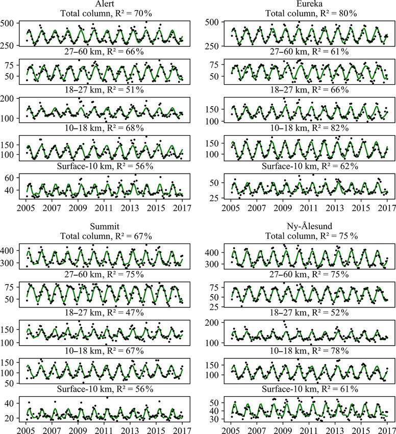
9734                                                           S. Bahramvash Shams et al.: Variations in high-latitude ozone

Holton et al., 1995; Kivi et al., 2007; Rao et al., 2004;           fully understand the variability in ozone concentrations. This
Rex, 2004) and photolysis involving photochemical reactions         situation is exacerbated by both the lack of high temporal ob-
(Yang et al., 2010) and climate variables (Rex, 2004). Stud-        servations at high latitudes as well as the difficulty of making
ies show that the mean total column ozone (TCO) decreased           quality measurements during winter; many ground-based and
from 1997 to 2003 globally (e.g., Newchurch, 2003), but             spaceborne remote-sensing instruments for measuring ozone
some reports show that the rate of ozone depletion has re-          depend on solar radiation (Bowman, 1989; Hasebe, 1980;
cently decreased due to the ramifications of the Montreal           Vigouroux et al., 2008, 2015). The Microwave Limb Sounder
Protocol (Weatherhead and Andersen, 2006; WMO, 2014;                (MLS) is a spaceborne instrument that measures atmospheric
Steinbrecht et al., 2017; Weber et al., 2018). However, re-         emission, which makes it capable of retrieving ozone over
cent work shows evidence of decreases in lower-stratospheric        the Arctic (Waters et al., 2006). This capability motivates the
ozone from 1998 to 2016 over 60◦ N to 60◦ S (Ball et al.,           use of MLS retrievals for analysis of stratospheric ozone in
2018). Because of these changes, it is important to monitor         the Arctic (Manney et al., 2011; Kuttippurath et al., 2012;
ozone variability at many locations globally and to under-          Wohltmann et al., 2013; Livesey et al., 2015; Strahan and
stand the causes of the variability.                                Douglass, 2018).
   During winters with persistent westerly zonal winds over            One of the most important and reliable instruments for
the tropics, planetary-scale Rossby waves modulate strato-          measuring the vertical profile of ozone is the ozonesonde.
spheric circulation. Stratospheric circulation is related to        These instruments can be launched year-round and can
the tropical quasi-biennial oscillation (QBO; Ebdon, 1975;          provide valuable information for the validation of remote-
Holton and Tan, 1980). The interactions of planetary-scale          sensing instruments aboard satellites. The Global Monitor-
Rossby waves and the QBO in the stratosphere modulate a             ing Division (GMD) of the National Oceanic and Atmo-
meridional mass circulation towards the polar regions called        spheric Administration (NOAA), Environment and Climate
the Brewer–Dobson circulation (Lindzen and Holton, 1968;            Change Canada, and the Helmholtz Centre for Polar and Ma-
Holton and Lindzen, 1972; Wallace, 1973; Holton et al.,             rine Research launch ozonesondes routinely in the Arctic.
1995). The location of the zero-wind line (latitude where the       Ozonesondes have used the data to study trends, patterns,
zonal wind speed is zero relative to the ground) is an impor-       and the vertical distribution of ozone from many locations
tant indicator of the strength of this circulation (Holton and      (Logan, 1994; Steinbrecht et al., 1998; Logan et al., 1999;
Lindzen, 1972; Holton and Tan, 1980). During the easterly           Solomon et al., 2005; Miller et al., 2006). Ozonesonde pro-
phase of the QBO, the zero-wind line shifts north, facilitat-       files from various Arctic stations have been used to study the
ing the propagation of planetary waves into the Arctic polar        climatology of the ozone cycle (Rao et al., 2004), the vertical
vortex. This creates a weakening of the vortex that increases       distribution of ozone and its dependence on different proxies
the transport of relatively warm, ozone-rich air into the Arctic    (Rao, 2003; Tarasick, 2005; Kivi et al., 2007; Gaudel et al.,
(Holton and Tan, 1982). The warmer temperatures are associ-         2015), trends and annual cycles of ozone (Christiansen et al.,
ated with decreased occurrence of polar stratospheric clouds        2017), the variability in ozone due to climate change (Rex,
(PSCs) and consequently fewer heterogeneous reactions in-           2004), ozone loss and the relation to dynamical parameters
volving the PSCs, which lead to less photochemical ozone            (Harris et al., 2010), and the difference of ozone depletion
loss in the stratosphere (Rex, 2004; Shepherd, 2008). Con-          in the Arctic and Antarctic (Solomon et al., 2014) and to
versely, during the westerly phase of the QBO, the propaga-         validate other sensor measurements (McDonald et al., 1999;
tion of planetary waves between the tropics and the Arctic          Vigouroux et al., 2008; Ancellet et al., 2016).
decreases, and the polar vortex is strengthened, resulting in          The sector of the Arctic from 0 to 60◦ W is known to
lower temperatures and increased probability of photochem-          be very sensitive to dynamical processes (see Fig. 2a of
ical ozone loss. Thus, dynamical processes and the state of         Antsey and Shepherd, 2014). In spite of this, the long record
the polar vortex are important factors that determine ozone         of ozonesonde launches (2005–2017) by NOAA GMD has
amounts in the Arctic.                                              never been used to study the long-term variability in tropo-
   Although there is strong observational evidence to sup-          spheric and stratospheric ozone over Summit Station, Green-
port this teleconnection between the tropical and Arctic at-        land (72.6◦ N, 38.4◦ W; 3200 m). Summit Station is located
mosphere, a complete theoretical explanation has proved dif-        in central Greenland atop the Greenland ice sheet (GrIS)
ficult (Anstey and Shepherd, 2014). The interaction of the          and is the drilling site of the Greenland Ice Sheet Project 2
background zonal mean wind and planetary waves is not               (GISP2) ice core. Ny-Ålesund, Svalbard, Norway, and Alert
completely understood, which makes it difficult to ascribe,         and Eureka, Nunavut, Canada, are high-latitude stations in
in detail, how atmospheric dynamics affect the polar vor-           this section of the Arctic that also routinely launch ozoneson-
tex. Furthermore, these effects depend on location and can          des.
also affect different portions of the atmosphere (Staehelin            In this study, we use 12 years of ozonesonde measure-
et al., 2001; Rao, 2003; Rao et al., 2004; Yang et al., 2006;       ments (from 2005 to 2017) to document the vertical structure
Vigouroux et al., 2008, 2015). Thus, detailed analyses of the       of ozone at high-latitude sites in the Arctic. In Sect. 2, we de-
vertical structure of ozone are needed at various locations to      scribe how ozone profiles over these sites are constructed us-

Atmos. Chem. Phys., 19, 9733–9751, 2019                                              www.atmos-chem-phys.net/19/9733/2019/
S. Bahramvash Shams et al.: Variations in high-latitude ozone                                                              9735

                                                                 studied to have a consistent dataset at all stations. The time
                                                                 period is also constrained by the availability of MLS data,
                                                                 which have been available since 2004. The ozonesonde pro-
                                                                 files from Summit Station are available from NOAA’s Earth
                                                                 System Research Laboratory, while the profiles from the
                                                                 Canadian stations and Ny-Ålesund can be found at the World
                                                                 Ozone and Ultraviolet Radiation Data Centre (WOUDC).
                                                                 The ozonesondes used here utilize electrochemical concen-
                                                                 tration cells (ECCs; Komhyr, 1969), manufactured by either
                                                                 Science Pump for Ny-Ålesund or Environmental Science
                                                                 (EN-SCI) for Summit, Alert, and Eureka. The ozonesondes
                                                                 at Ny-Ålesund, Alert, and Eureka used a sensing solution of
                                                                 neutral buffered 1 % potassium iodide, while the ozoneson-
                                                                 des at Summit used a reduced (one-tenth) buffer concentra-
                                                                 tion. The data records of the Canadian sites have recently
                                                                 been re-evaluated (Tarasick et al., 2016), as has the Summit
                                                                 record (Sterling et al., 2018). Based on the ozone sensor re-
                                                                 sponse time of 25–40 s (Smit and Kley, 1998), and assum-
Figure 1. Map showing the locations of study sites used: Sum-    ing a typical balloon ascent rate of 4–5 m s−1 , the ozoneson-
mit Station, Greenland; Ny-Ålesund, Svalbard, Norway; Alert,
                                                                 des have a vertical resolution of about 100–200 m. The mea-
Nunavut, Canada; and Eureka, Nunavut, Canada.
                                                                 surement precision is ±3 %–5 %, and the overall uncertainty
                                                                 in ozone concentration in parts per million volume is from
ing data from both ozonesondes and satellite retrievals from     about ±10 % up to 30 km (Komhyr, 1986; Komhyr et al.,
the MLS. This section also describes the data screening that     1989; Kerr et al., 1994; Johnson et al., 2002; Smit et al.,
was performed on these measurements. Section 3 discusses         2007; Deshler et al., 2008, 2017).
the methods used in the data analysis, including determina-         We use retrievals from the MLS (version 4.2) above the
tion of the seasonal cycle and the stepwise multiple regres-     maximum height of each ozonesonde up to 60 km. The MLS
sion (SMR) technique (Appenzeller et al., 2000; Brunner et       is an instrument on the Aura spacecraft that uses microwave
al., 2006; Kivi et al., 2007; Vigouroux et al., 2015; Stein-     emission to measure atmospheric composition, temperature,
brecht et al., 2017). Stepwise multiple regression is used       and cloud properties (Waters et al., 2006). Ozone retrievals
to determine the drivers of ozone variations at each of the      from the MLS have been available continuously since 2004
sites. Section 4 presents the results of this study, including   over the Arctic, with overpasses over these sites every few
the seasonal cycles, trends, and variations in total column      days. The standard MLS ozone product, which is retrieved
ozone (TCO) and partial column ozone (PCO) in four atmo-         from spectra with frequency 240 GHz, is used in this study.
spheric layers: the troposphere and the lower, middle, and up-   The column value uncertainty (σ ) is 2 % to 3 % (Livesey et
per stratosphere. This section also determines the important     al., 2018). The vertical resolution of the MLS profiles is from
drivers of the deseasonalized ozone data (based on various       100 to 22 hPa is 2.5 km and increases to 3 km in both the
proxies using stepwise multiple regression) that are common      lower and upper stratosphere (Livesey et al., 2017). The MLS
to all of the four sites. These drivers are then used to cre-    ozone products have previously been used in ozone analyses,
ate final models of ozone variations. Section 5 presents the     e.g., for polar ozone loss (Manney et al., 2011; Kuttippurath
conclusions of this research study.                              et al., 2012; Wohltmann et al., 2013; Livesey et al., 2015;
                                                                 Strahan and Douglass, 2018).
                                                                    Data screening was performed on each ozonesonde used
2   Data                                                         in this study. Figure 2 shows a histogram of the maximum
                                                                 height of the ozonesondes for the entire 12-year period at all
Summit Station, Greenland (72◦ N, 39◦ W); Ny-Ålesund,            study locations. Most of the ozone profiles have maximum
Svalbard, Norway (79◦ N, 12◦ E); Alert, Canada (82◦ N,           heights of 25 km or greater, but there is a significant fraction
62◦ W; and Eureka, Canada (70◦ N, 86◦ W), are chosen as          with maximum heights below 25 km. A bi-modal distribution
the study sites for this research because there is a long his-   is apparent at all stations except Ny-Ålesund and is caused
tory of ozonesonde observations at these locations. Figure 1     partly by the fact that the burst altitude of the balloons de-
shows the locations of these stations in the Arctic.             pends on season; lower maximum altitudes are achieved in
   Summit Station ozone measurements were started in             the extreme cold experienced during winter. The MLS has
February 2005 and continued until the summer of 2017. The        high uncertainty in the lower atmosphere. Thus, to minimize
other stations have longer datasets, but in this study, 12 an-   the uncertainty in the calculation of TCO, ozonesondes that
nual cycles from February 2005 through February 2017 are         reached a maximum height of greater than 12 km were used

www.atmos-chem-phys.net/19/9733/2019/                                             Atmos. Chem. Phys., 19, 9733–9751, 2019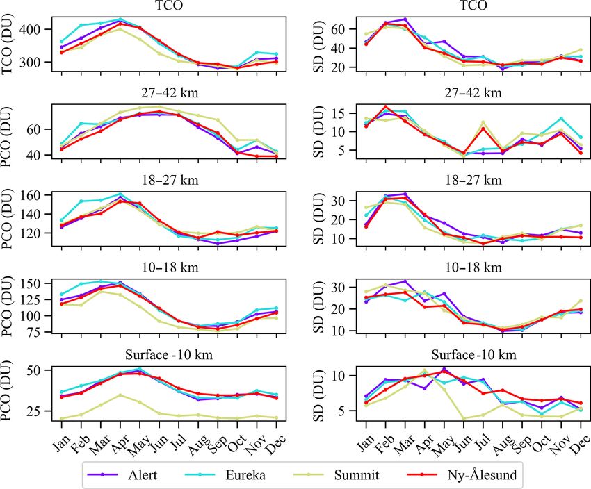
9736                                                           S. Bahramvash Shams et al.: Variations in high-latitude ozone

Figure 2. Maximum height reached by ozonesondes launched at
Alert, Nunavut, Canada; Eureka, Nunavut, Canada; Summit Station,
Greenland; and Ny-Ålesund, Svalbard, Norway, between Febru-
ary 2005 and February 2017.

in this study; profiles with maximum heights below 12 km
were eliminated from further analysis. The fraction of TCO
below 12 km (∼ 200 hPa) at these sites is about 13 %–17 %.
   Another data-screening issue is related to missing data in       Figure 3. The difference in total column ozone (TCO) calculated
the ozonesonde profiles. Most of the missing values occur at        using profiles from the Microwave Limb Sounder (MLS) only ver-
high altitudes because the ozonesonde ceased to report valid        sus profiles using ozonesonde in the lower atmosphere and MLS in
measurements. There were also some missing data between             the upper atmosphere. The differences are calculated as MLS only
valid ozone measurements. In this study, profiles that have a       minus the ozonesonde and MLS for Alert, Eureka, Summit, and
percentage of missing data greater than 40 % are eliminated         Ny-Ålesund.
from further analysis. In the remaining profiles, if missing
values occurred between valid ozone measurements, the pro-
file was linearly interpolated to fill the missing data. After      ally defined by the Dobson unit (DU), which is the thick-
applying the data screening, more than 25 ozonesondes are           ness of a compressed gas in the atmospheric profile in
retained for analysis in each month for the 12-year period,         units of 10 µm at standard temperature and pressure; 1 DU
which satisfies the requirement for calculating a meaningful        is equivalent to 1 milli-atmosphere centimeter or 2.69 ×
monthly mean profile (Logan et al., 1999).                          1016 molecules cm−2 . Merged ozonesondes up to 60 km pro-
   Ozone profiles in this study are constructed by merging the      vide an appropriate dataset to integrate over all layers of the
ozonesondes up to the burst altitude (Fig. 2) and then using        atmosphere that contain appreciable ozone. In this study, the
the MLS profiles up to 60 km. The merged profiles are gener-        PCO amounts are calculated for the following altitude re-
ated only if an MLS ozone profile is within a 2◦ ×2◦ latitude–      gions: surface to 10, 10 to 18, 18 to 27, and 27 to 60 km.
longitude grid cell around each station and within 4 d of the       For the purpose of this study, the layers represent the tro-
ozonesonde launch. The majority of the merged profiles are          posphere, lower stratosphere, middle stratosphere, and upper
generated using MLS data on the day of the launch or within         stratosphere, respectively. Note that the tropopause is low in
1 d of the launch. Figure 3 shows the difference of TCO from        the Arctic, so the layer from the ground to 10 km represents
the merged ozone profile versus TCO from the MLS only at            primarily values in the troposphere but also contains some
all stations. This shows that the MLS mostly overestimates          ozone from the lowest portion of the stratosphere. However,
the ozone in the lower atmosphere at all stations. Thus, the        we refer to this layer here as the “troposphere” for conve-
merged profile dataset minimizes the uncertainty in ozone at        nience.
these sites by using the more accurate ozonesonde data for as          SMR has been widely used in the past (e.g., Appenzeller
much of the lower atmosphere as possible.                           et al., 2000; Brunner et al., 2006; Kivi et al., 2007; Mäder
                                                                    et al., 2007; Vigouroux et al., 2015) for selecting impor-
                                                                    tant variables that affect ozone concentrations. Wohltmann
3   Methods                                                         et al. (2007) explain some of the issues with using multiple
                                                                    regression to determine atmospheric ozone variations. How-
The total amount of ozone in the vertical profile is a              ever, this technique can be inaccurate if there is spurious cor-
useful parameter for understanding ozone variations in              relation between the different variables and the deseasonal-
the atmosphere. The ozone column density is tradition-              ized ozone time series (Wohltmann et al., 2007). In this study,

Atmos. Chem. Phys., 19, 9733–9751, 2019                                              www.atmos-chem-phys.net/19/9733/2019/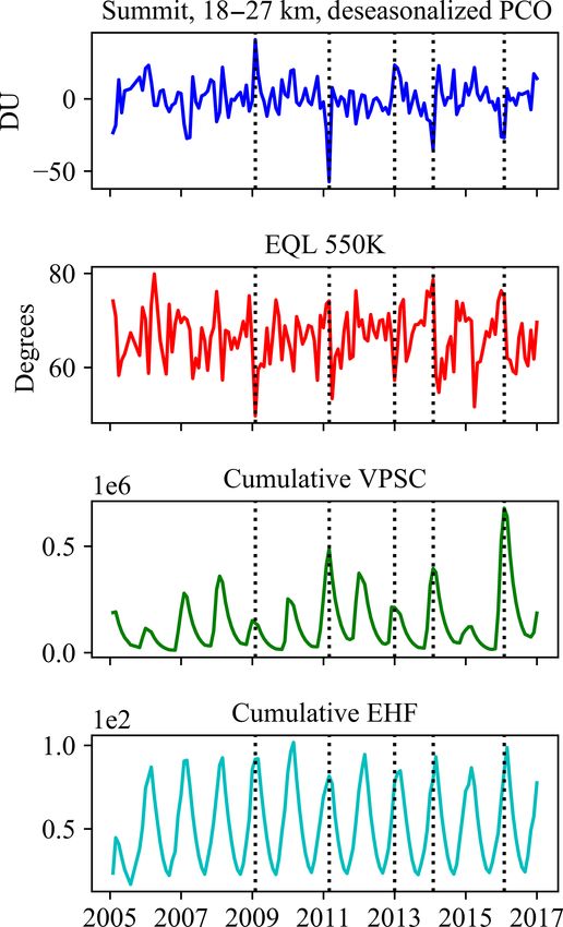
S. Bahramvash Shams et al.: Variations in high-latitude ozone                                                                                          9737

we use a combination of SMR and the “process-based” ap-                                      fit to the time series using multiple linear regression to cre-
proach of Wohltmann et al. (2007) to determine the impor-                                    ate a new time series. This process is repeated until none of
tant drivers of ozone variations at the Arctic sites. In partic-                             the remaining proxies increase the R 2 by more than 1 %. The
ular, SMR is used to determine a set of physical parameters                                  final set of drivers of Arctic ozone in each layer, as well as
that are important at three or more of the sites and are, there-                             the TCO, are defined as those that are common among three
fore, common drivers of ozone variations in the Arctic. These                                or more sites, based on the SMR analysis. These proxies are
variables are then used to derive final models for PCO in each                               then used to create a final model for PCO and TCO, as de-
of the four atmospheric layers and for TCO at each site. This                                scribed in Sect. 4.4.
procedure then reduces the effect of spurious correlations be-
tween variables and deseasonalized ozone time series that is
experienced when using SMR only.                                                             4     Results and discussion
   The general approach is briefly explained here, while the
analysis and results are discussed below in Sect. 4. First, the                              In this section, the 12-year records of ozonesonde profiles
SMR uses various proxies that have been previously identi-                                   over the four Arctic stations are discussed. First, the seasonal
fied as important indicators of ozone concentrations in the                                  cycles of ozone at the four sites are compared. The trends of
troposphere and stratosphere. Figure 4 shows time series of                                  ozone in various vertical sections of the atmosphere are also
the proxies: tropopause pressure (TP); the QBO at both 10                                    discussed. Finally, we describe the results of the SMR anal-
and 30 hPa (QBO10; QBO30); the volume of polar strato-                                       ysis and the final ozone models, which yield insight into the
spheric clouds (VPSC); eddy heat flux (EHF); Arctic oscilla-                                 primary drivers of ozone variability over four Arctic stations.
tion (AO); equivalent latitude (EQL) at three potential tem-
perature levels, 370, 550, and 960 K; solar flux (SF); and the                               4.1    Seasonal cycle
El Niño–Southern Oscillation index (ENSO). The monthly
averaged values for TP and AO are calculated using data for                                  To examine the seasonal cycle at each station, the monthly
the same dates as the ozonesonde launches for each station.                                  averaged TCO and PCO are calculated. The TCO (and the
EQL, TP, and AO are estimated at each station. In Fig. 4,                                    PCO amounts) depends on both temperature and pressure,
EQL, TP, and AO at Summit Station are shown as examples.                                     so differences in the profiles of these variables over the dif-
Table 1 lists the data sources and weblinks of these proxies.                                ferent sites will affect the column ozone. Figure 5 shows the
This list is similar to that used by previous studies (Brunner                               multi-year monthly averages (left column) and the associated
et al., 2006; Vigouroux et al., 2015). Following Vigouroux                                   standard deviations (right column) of TCO (top row) and the
et al. (2015), the stepwise multiple regression model is given                               PCO amounts for the four atmospheric layers. The total col-
by                                                                                           umn ozone reaches its peak value in April for all stations.
                                                                                       The minimum value of TCO at all sites occurs in September
                           2πt                      2πt                      4πt             or October. The ozone values in the upper stratosphere fluc-
Y (t)= A0 + A1 cos                   + A2 sin                 + A3 cos
                            12                       12                       12             tuate between 40 and 80 DU for all stations. The largest val-

                    4π t           Xn                                                        ues of PCO occur in the layers of the middle (120–160 DU)
     + A4 sin                  +       k=5
                                             Ak X(t)k + ε (t) ,                        (1)   and lower stratosphere (75–150 DU). The PCO in the tropo-
                     12
                                                                                             sphere ranges from about 20 to 35 DU at Summit Station and
where Y (t) is the final regression model, t is the month (1 to                              from 35 to 50 DU at the other stations. These values are lower
12), A0 –A4 are coefficients related to the seasonal cycle, Ak                               at Summit Station due to its high surface elevation of about
(for k ≥ 5) is the coefficients related to the proxy time series                             3200 m.
X(t)k , and ε is the residual ozone that is not explained by                                    The seasonal cycles of TCO show significant differences
the combination of the seasonal cycle and the proxies. Any                                   at the four sites. The cycles at Alert and Eureka are simi-
linear trend in the data is considered to be one of the proxies                              lar, but Eureka exhibits slightly larger values than Alert from
using Xk (t) = t. The model is implemented using the follow-                                 November to March. The differences between these two sites
ing procedure. First, the seasonal cycle for the 12-year pe-                                 are somewhat surprising given the close proximity of the
riod is determined by finding the coefficients A0 –A4 . These                                two stations. The TCO values at Ny-Ålesund are larger than
terms are then subtracted from the original TCO time series                                  any other site from May to August but then exhibit the low-
to yield deseasonalized time series. Using the technique de-                                 est TCO in winter (November–January). The TCO values
scribed in Sect. 7.4.2 of Wilks (2011), stepwise regression                                  at Summit are the lowest of any of the sites in May, June,
(with forward selection) is then performed on the deseason-                                  and July. The seasonal cycle of the standard deviations in the
alized time series using the different proxies. To accomplish                                TCO are similar at all the sites, with maximum values in late
this, each proxy is regressed with the deseasonalized TCO                                    winter and early spring and minimum values in fall.
and PCO time series, and the proxy that has the highest ex-                                     The seasonal cycles are also quite different in the various
plained variance (R 2 ) and a p value lower than 0.05 is se-                                 atmospheric layers. The timing of the peak ozone at differ-
lected. This proxy (e.g., A5 X5 (t)) is then included in a new                               ent altitudes is due to different physical processes that affect

www.atmos-chem-phys.net/19/9733/2019/                                                                         Atmos. Chem. Phys., 19, 9733–9751, 2019
9738 S. Bahramvash Shams et al.: Variations in high-latitude ozone Figure 4. Time series of the proxies used in this study to analyze ozone variations over Summit Station, Greenland. The sources of the proxies are listed in Table 1. The units of the proxies are unitless for ENSO and AO; meters per second for QBO10 and QBO30 (positive values are westerly zonal winds, and negative values are easterlies), watts per square meter for solar flux and eddy heat flux (EHF), hectopascals for tropopause pressure (TP), 106 km3 for volume of polar stratospheric clouds (VPSC), and degrees for equivalent latitude (EQL) at potential temperatures of 370, 550, and 960 K. The proxy for VPSC is actually the cumulative volume of polar stratospheric clouds times the effective equivalent stratospheric chlorine (EESC), and cumulative EHF is named EHF (Brunner et al., 2006), as explained in the text. The proxies for TP and EQL are for Summit Station. ozone concentrations. In the upper stratosphere (27–42 km), TCO, the PCO values at Ny-Ålesund remain elevated (rel- the values are about 30 to 40 DU higher in spring than the ative to the other sites) through most of the summer until minimum in the fall due to increased sunlight in spring, when August. This springtime maximum is due to accumulation photolysis equilibrium is reached (Crutzen, 1971). For all of transported ozone from lower latitudes during wintertime stations, the PCO values in this layer peak later in the year caused by the Brewer–Dobson circulation (Staehelin et al., than the TCO, with values of about 75–80 DU in May, June, 2001). The PCO is largest at Eureka from November to April. and July. The PCO is slightly higher in most months at Sum- All stations show similar standard deviations in this layer, mit Station compared to the other stations. The standard de- with the largest fluctuations in winter and spring. viations in the upper stratosphere are similar at all stations, The PCO in the lower stratosphere peaks in March at Sum- except for Summit and Ny-Ålesund, which have larger vari- mit Station and Eureka and in April at Ny-Ålesund and Alert. ability than Alert and Eureka in June. This pattern represents the well-known springtime maximum The PCO in the middle stratosphere peaks earlier in spring in the Arctic, which is caused by winter ozone accumulation than in the upper stratosphere, peaking in April at Alert, Eu- that occurs before ozone is transported to the troposphere reka, and Summit and in May at Ny-Ålesund. Similar to the (Rao, 2003; Rao et al., 2004; Staehelin et al., 2001). Sum- Atmos. Chem. Phys., 19, 9733–9751, 2019 www.atmos-chem-phys.net/19/9733/2019/
S. Bahramvash Shams et al.: Variations in high-latitude ozone                                                                             9739

Table 1. Proxies used in the stepwise multiple regression performed in this study to explain variance in the total column ozone amount.

                                              Description                                  Source
   Tropopause pressure (TP)                   Derived from NCEP–NCAR reanalysis            https://www.esrl.noaa.gov/psd/cgi-bin/
                                              data from NOAA’s Earth System Re-            db_search/DBListFiles.pl?did=195&tid=
                                              search Laboratory                            74737&vid=679 (last access: 22 July 2019)
   Quasi-biennial oscillation (QBO)           Based on equatorial stratosphere winds       https://www.geo.fu-berlin.de/met/ag/strat/
                                              at 30 and 10 hPa                             produkte/qbo/singapore.dat
                                                                                           (last access: 22 July 2019)
   Volume polar stratospheric clouds          Calculated between 375 and 550 K po-         Calculated at FMI using chemistry and trans-
   (VPSC)                                     tential temperature                          port model FinROSE (Damski et al., 2007)
   Eddy heat flux (EHF)                       Averaged over 45–75◦ N at 100 hPa            https://acd-ext.gsfc.nasa.gov/Data_services/
                                                                                           met/ann_data.html (last access: 22 July 2019)
   Arctic oscillation (AO)                                                                 https://www.cpc.ncep.noaa.gov/products/
                                                                                           precip/CWlink/daily_ao_index/ao.shtml
                                                                                           (last access: 22 July 2019)
   Equivalent latitude (EQL)                  At three altitude levels of potential tem-   Calculated at FMI
                                              peratures of 370, 550, and 960 K
   EESC                                       Mean age of air 5.3 years                    https://acd-ext.gsfc.nasa.gov/Data_services/
                                                                                           automailer/restricted/eesc.php
                                                                                           (last access: 22 July 2019)
   Solar flux                                                                              ftp://ftp.ngdc.noaa.gov/STP/space-weather/
                                                                                           solar-data/solar-features/solar-radio/
                                                                                           noontime-flux/penticton/penticton_observed/
                                                                                           tables/table_drao_noontime-flux-observed_
                                                                                           monthly.txt (last access: 22 July 2019)
   Multivariate ENSO index (MEI)                                                           https://www.esrl.noaa.gov/psd/enso/mei/

mit Station has lower PCO values in this layer from April                 4.2   Trends
to September. The springtime decline in ozone over Summit
appears to start earlier (in March), and then the ozone re-               The temporal trends in the TCO and PCO at all four stations
mains low until October. The PCO at Ny-Ålesund has a large                are now considered. Linear regression is performed on the
range, with minimum values similar to Summit Station in fall              time series to determine the temporal trends. For a trend to
but maximum values due to wintertime accumulation that are                be significant, the slope of the regression line must be greater
similar to Alert and Eureka.                                              than the standard error in the slope by 0.1 DU yr−1 . The de-
   Eureka and Alert have very similar seasonal cycles of tro-             tails of the trend analysis can be found in Figs. S1–S5 and
pospheric ozone, reaching a maximum in May and minimum                    Table S1 in the Supplement.
in August. On the other hand, the PCOs at Summit Station                     The trends were calculated for the 12-year period using
and Ny-Ålesund peak in April and June. As expected, the                   annual, spring (MAM), summer (JJA), fall (SON), and win-
ozone fluctuations in this layer are small. In general, the stan-         ter (DJF) values. There is no significant trend in the an-
dard deviations in tropospheric PCO are smallest at Summit                nual values of the TCO or any of the PCO values at any
Station, likely due to the lower PCO values. The peak in the              of the stations. Ny-Ålesund and Summit Station are the
tropospheric PCO in spring is caused primarily by relatively              only sites that have significant seasonal trends. In spring,
large ozone concentrations between 6 and 10 km. The peak in               Ny-Ålesund has a negative trend in both the troposphere
the upper troposphere is likely caused by intrusion of ozone-             (−0.7 ± 0.5 DU yr−1 ) and the upper stratosphere (−1.0 ±
rich air from the stratosphere. The subsequent intrusion of               0.6 DU yr−1 ). In summer, Summit has a negative trend in the
ozone into the troposphere later in the spring is likely the              upper stratosphere (−0.4 ± 0.2 DU yr−1 ), and Ny-Ålesund
result of tropospheric folds that occur in mid-spring to late             has relatively large positive trends in the troposphere (+0.7±
spring (Holton et al., 1995; Walker et al., 2012; Tarasick et             0.2 DU yr−1 ), lower stratosphere (+2.6±0.9 DU yr−1 ), mid-
al., 2019).                                                               dle stratosphere (+1.5 ± 0.5 DU yr−1 ), and in the total col-
                                                                          umn (+4.9 ± 1.4 DU yr−1 ). In fall, Ny-Ålesund has signifi-

www.atmos-chem-phys.net/19/9733/2019/                                                       Atmos. Chem. Phys., 19, 9733–9751, 2019
9740 S. Bahramvash Shams et al.: Variations in high-latitude ozone
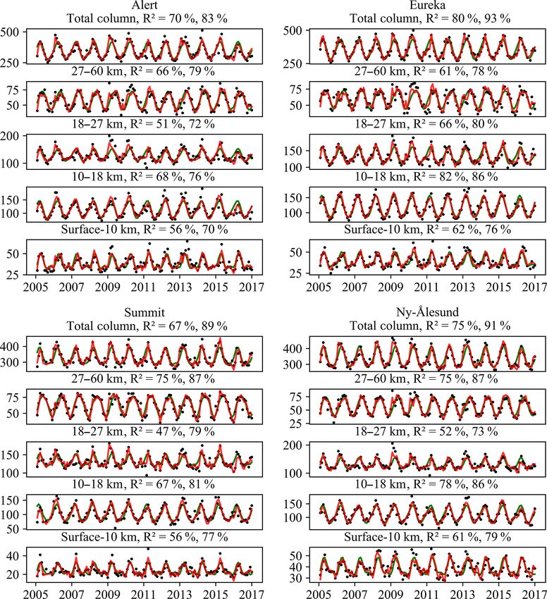
Figure 5. Monthly mean (left panels) and standard deviations (right panels) of total column ozone (TCO) and partial column ozone (PCO)
for 2005–2017 for different atmospheric layers from merged ozonesonde and MLS for Alert, Eureka, Summit, and Ny-Ålesund. The layers
represent the troposphere (surface–10 km), the lower stratosphere (10–18 km), the middle stratosphere (18–27 km), and the upper stratosphere
(27–42 km). The TCO is calculated from the surface to 60 km.
cant trends in all the stratospheric layers, but the trend is pos- four altitude regions (bottom four panels) for each station.
itive in the upper stratosphere (+1.4±0.2 DU yr−1 ) and neg- The seasonal cycles are also shown in Fig. 6 as the green
ative in the middle stratosphere (−0.6±0.3 DU yr−1 ) and the curves. The values of the correlation of determination (R 2 )
lower stratosphere (−1.3 ± 0.5 DU yr−1 ). In fall, Summit ex- are shown above each panel and represent the variance in the
hibits negative trends in both the TCO (−1.8 ± 1.1 DU yr−1 ) original time series that is explained by the seasonal cycle.
the middle stratosphere (−0.9 ± 0.6 DU yr−1 ). These values are also shown in Table 2 for comparison. The
In summary, Alert and Eureka have no significant trends in seasonal cycle explains over 50 % of the variance in both the
ozone. There are a few significant trends at Summit Station in total and partial column ozone values at all stations except
summer and fall that are all negative. Ny-Ålesund has trends the middle stratosphere at Summit Station (47 %) and Ny-
in spring, summer, and fall, with the large positive trends in Ålesund (38 %). The R 2 value for TCO is highest at Eureka
summer and mostly small negative trends in spring and fall. (0.80) and lowest at Ny-Ålesund (0.65). Because the seasonal
cycle explains a high percentage of the ozone fluctuations
4.3 Drivers of ozone variation over Greenland over Eureka, this site may be less susceptible to dynamical
and chemical perturbations compared to the other sites. By
To identify the drivers of ozone variations, the SMR tech- comparing the R 2 values in the different atmospheric layers,
nique described in Sect. 3 is used. We refer back to Fig. 4, we see that the middle stratosphere has the lowest R 2 at all
which describes the proxies used for SMR. The most dom- the stations except Eureka. This shows that the ozone in the
inant source of ozone variation is the seasonal cycle, so the middle stratosphere at these Arctic sites is more susceptible
first step in the analysis is to remove this cycle. To remove to perturbations than other layers.
the seasonal cycle, we first fit the TCO and PCO time se- By examining the difference between the original time
ries using the first five terms in Eq. (1) (using coefficients series (black dots) and the seasonal cycles (green lines) in
A0 –A4 ). The derived seasonal cycle is then subtracted from Fig. 6, we can see that there is additional variance that re-
the original time series to create a deseasonalized time se- mains unexplained. This is motivation to conduct the SMR
ries. Figure 6 shows the values of total column ozone (top analysis to identify the most important drivers that are com-
panels) and the partial ozone column values for each of the
Atmos. Chem. Phys., 19, 9733–9751, 2019 www.atmos-chem-phys.net/19/9733/2019/S. Bahramvash Shams et al.: Variations in high-latitude ozone 9741 Figure 6. Time series of the total column ozone (top panels) and the partial column ozone (black dots) in four atmospheric layers (four bottom panels) from Alert, Eureka, Summit, and Ny-Ålesund. The fitted seasonal cycle is shown as the green curves. The coefficient of determination (R 2 ) for each seasonal fit is shown in the title for each panel. mon at the four Arctic sites. To accomplish this, the SMR lation of determination. We also list the sign of the slope of analysis is performed on the deseasonalized time series. Be- the regression fit of each proxy in Table 3 to the left of the R 2 fore the results of the SMR analysis are discussed, it is im- value (except for the QBO because this proxy involves multi- portant to note that the removal of the seasonal cycle likely ple terms); the sign of the slope indicates positive or negative decreases the influence of proxies that have seasonal varia- correlation between the proxy and the deseasonalized time tions. Figure 4 shows that this is mostly true for the eddy heat series. The bottom row of Table 3 lists the cumulative R 2 flux and, to a lesser degree, the volume of polar stratospheric value of all selected proxies. The time trends were included clouds. in the regression analysis by using Ak = 1 in Eq. (1). The SMR analysis is initiated by calculating the coeffi- To identify the most important proxies that affect Arc- cient of determination (R 2 ) for each proxy. The best proxy tic ozone (to be used in our final model), we use proxies at each step in the analysis is the one with the largest R 2 that are selected at three or more of the four sites. Table 4 value, which is at least 1 % higher than the R 2 of the pre- shows that tropopause pressure (TP) is the most important vious step. These fits must also have a p value of less than proxy for TCO and tropospheric PCO at all of the stations. 0.05 to be considered in the analysis. Table 3 summarizes the The seasonal cycle in TP is difficult to detect in Fig. 4a, results for each time series. (More detailed information, such but the largest values of TP generally occur in winter and as the regression slopes and standard errors of the slope, can spring; note that the y axis in Fig. 4a decreases upward, so be found in Tables S2–S5 of the Supplement.) The lists of large pressure values indicate lower height levels in the at- proxies are in descending order of contribution to the corre- mosphere. TP has been shown to correlate well with total www.atmos-chem-phys.net/19/9733/2019/ Atmos. Chem. Phys., 19, 9733–9751, 2019
9742                                                             S. Bahramvash Shams et al.: Variations in high-latitude ozone

Table 2. Correlation of determination (R 2 in %) for the seasonal cycle, stepwise regression model (SMR), and the final model of ozone
variations (February 2005–February 2017). The improvement in the correlation of determination between the seasonal cycle and final models
is shown as 1 for each station. The text is in bold when the improvement is higher than 20 %.

                                             Surface–10 km     10–18 km     18–27 km     27–42 km     Total column
                     Alert
                     Seasonal cycle model                 57           68          51           66               70
                     SMR                                  75           76          75           81               84
                     Final model                          70           76          72           79               83
                     1                                    14            8          21           13               13
                     Eureka
                     Seasonal cycle model                 62           82          66           61               80
                     SMR                                  77           91          87           84               94
                     Final model                          76           86          80           78               93
                     1                                    14            4          14           17               13
                     Summit
                     Seasonal cycle model                 56           67          47           75               67
                     SMR                                  78           87          80           87               89
                     Final model                          77           81          79           87               89
                     1                                    21           14          32           12               22
                     Ny-Ålesund
                     Seasonal cycle model                 52           70          38           67               65
                     SMR                                  64           79          66           76               81
                     Final model                          64           79          55           75               80
                     1                                    12            9          17            8               15

column ozone (Appenzeller et al., 2000; Steinbrecht et al.,            ations in the middle and upper stratosphere, while the EQL
1998). Lower TP (higher tropopause height) leads to lower              at 370 K is found to have an important influence on tropo-
values of ozone (Steinbrecht et al., 1998). Tropopause height          spheric ozone at these sites.
can also be increased due to lower stratosphere temperatures              The Brewer–Dobson circulation is one of the most impor-
(Forster and Shine, 1997), which can result in ozone deple-            tant processes of ozone transport from the tropics to the Arc-
tion (Rex, 2004). The transport of ozone to higher levels in           tic (Staehelin et al., 2001). The seasonal cycle of ozone in the
the atmosphere can increase ozone destruction because pho-             extratropics is caused by this circulation (Fusco and Salby,
tochemical reactions increase (when sunlight is available;             1999). The vertical component of the Eliassen–Palm (EP)
Steinbrecht et al., 1998).                                             flux and the EHF are proportional to each other and are both
   Potential vorticity (PV) also affects the ozone concentra-          good indicators of the Brewer–Dobson circulation (Brunner
tion. Equivalent latitude (EQL) is an index estimated based            et al., 2006; Eichelberger, 2005; Fusco and Salby, 1999). In
on PV that is indicative of ozone (air parcel) transportation          this study, the spatially averaged EHF at 100 hPa over 45–
on an isentropic level of potential temperature (Danielsen,            75◦ N is used. The variation in EHF is shown in Fig. 4e. As
1968; Butchart and Remsberg, 1986; Allen and Nakamura,                 mentioned above, the seasonal variation in EHF is similar to
2003). Adiabatic vertical movement of air parcels, caused              that of ozone over Summit Station, with maximum values in
by stratosphere–troposphere transport, changes the volume              winter. Large values of EHF indicate higher wave forcing of
of an air parcel. The mixing ratio is conserved in adiabatic           stratospheric circulation, which weakens the polar vortex and
movement; thus this transportation changes the density of              leads to higher ozone (Fusco and Salby, 1999); therefore, Ta-
ozone (Wohltmann et al., 2005). Moreover, horizontal advec-            ble 3 shows that the correlation between EHF and ozone is
tion on isentropic levels can affect the ozone concentration           positive. EHF is an important proxy of ozone in the Arctic
when there is an ozone gradient (Allen and Nakamura, 2003,             stratosphere (Tables 3 and 4).
Wohltmann et al., 2005). We use equivalent latitude at three              Heterogeneous reactions on the surfaces of the polar
potential temperature levels of 370, 550, and 960 K. Monthly           stratospheric clouds contribute to ozone depletion (Rex et al.,
fluctuations of these levels are shown in Fig. 4g, h, and i.           2004; Brunner et al., 2006). In this study, the volume of po-
The EQL at 550 K significantly influences Arctic ozone vari-           lar stratospheric clouds is multiplied by effective equivalent

Atmos. Chem. Phys., 19, 9733–9751, 2019                                                  www.atmos-chem-phys.net/19/9733/2019/
S. Bahramvash Shams et al.: Variations in high-latitude ozone 9743
Table 3. The correlation of determination (R 2 in %) obtained in the stepwise multiple regression analysis. The regression is performed on
the deseasonalized ozone time series. The R 2 values are listed in order of improvement in the descending order. Proxies that improve the R 2
by at least 1 % and that have a p value equal or less than 0.05 are added to model. The sign next to the R 2 value is the sign of the slope of
the regression. The R 2 of the final residual model for each atmospheric layer is shown in the bottom row. The sign of the QBO is not shown
because its contribution comes from several different terms, and a single slope sign is thus not applicable for this proxy. Extended tables for
each station can be found in the Supplement.
Alert
Surface–10 (km) 10–18 (km) 18–27 (km) 27–60 (km) Total column
Proxy R2 Proxy R2 Proxy R2 Proxy R2 Proxy R2
TP 19, + EHF 12, + EQL 17, – TP 16, + TP 19, +
QBO 6 VPSC 7, – EHF 12, + EHF 8, + EHF 8, +
AO 3, – QBO 1 VPSC 6, – AO 7, - VPSC 5, -
ENSO 3, – AO 4, – EQL 7, – EQL 4, –
Trend 3, + TP 3, + VPSC 5, – Solar 1, +
EQL 2, –
VPSC 1, –
Total R 2 37 20 43 34 37
Eureka
Surface–10 (km) 10–18 (km) 18–27 (km) 27–60 (km) Total column
Proxy R2 Proxy R2 Proxy R2 Proxy R2 Proxy R2
TP 20, + TP 20, + TP 30, + EQL 38 TP 37, +
QBO 5 AO 9, – EQL 15, – VPSC 7 EQL 7, –
EQL 4, – VPSC 8, – VPSC 8, – TP 3 VPSC 5, -
Trend 3, + Solar 4, + QBO 1 QBO 5
ENSO 2, – QBO 3
EQL 1, –
Total R 2 34 45 53 49 56
Summit
Surface–10 (km) 10–18 (km) 18–27 (km) 27–60 (km) Total column
Proxy R2 Proxy R2 Proxy R2 Proxy R2 Proxy R2
TP 36, + TP 35, + EQL 37, – EQL 39, – TP 34, +
EQL 1, – EQL 7, – VPSC 13, – EHF 4, + EQL 9, -
VPSC 7, – QBO 5 VPSC 2, – QBO 6
QBO 4 EHF 3, + VPSC 5, –
EHF 3, + EHF 5, +
AO 2, –
Total R 2 37 58 58 45 60
Ny-Ålesund
Surface–10 (km) 10–18 (km) 18–27 (km) 27–60 (km) Total column
Proxy R2 Proxy R2 Proxy R2 Proxy R2 Proxy R2
TP 12, + QBO 12 EHF 12, + EQL 8, – TP 18, +
QBO 3 EHF 9, + VPSC 11, – EHF 7, + EHF 11, +
EQL 2, – VPSC 6, – EQL 8, – AO 5, – VPSC 7, –
AO 4, – VPSC 2, – QBO 4
QBO 3 AO 3, –
TP 1, + EQL 2, –
Total R 2 17 27 39 22 45
www.atmos-chem-phys.net/19/9733/2019/ Atmos. Chem. Phys., 19, 9733–9751, 20199744 S. Bahramvash Shams et al.: Variations in high-latitude ozone
Table 4. The important drivers of ozone variations for each atmo- the QBO modulates planetary-scale Rossby waves and con-
spheric layer and for total column ozone (TCO). The drivers are sequently the poleward transport of ozone from the tropics by
tropopause pressure (TP), eddy heat flux (EHF), equivalent latitude shifting the zero-wind line. A close evaluation of the resid-
(EQL), volume of polar stratospheric clouds (VPSC), and the quasi- ual ozone and the QBO time series shows that the largest
biennial oscillation (QBO). The EQL at 370 K is used for surface ozone values occur when the QBO is in the easterly phase.
to 10 km, and the EQL at 550 K is used for the middle and upper
Under these conditions, the stratospheric circulation leads to
stratosphere.
increases in Arctic ozone by both weakening the polar vortex
and warming it up (Holton and Tan, 1980). In general, higher
Surface–10 10–18 18–27 27–60 TCO
(km) (km) (km) (km)
stratospheric temperatures in the Arctic lead to fewer PSCs,
√ √ which result in less photochemical loss of ozone (Rex, 2004;
TP Shepherd, 2008). On the other hand, the westerly phase of the
√ √ √ √
EHF QBO strengthens the polar vortex, which decreases strato-
√ √ √ √
EQL spheric temperatures over the Arctic and leads to ozone loss.
√ √ √ √
VPSC
√ √ √ The QBO significantly impacts ozone in the troposphere and
QBO
lower stratosphere at these Arctic sites (Tables 3 and 4).
The other proxies, the AO (Fig. 4f), solar flux (Fig. 4j),
and the ENSO (Fig. 4k), do not have a significant contribu-
stratospheric chlorine (EESC) to account for the modulation tion to ozone variations at these Arctic sites. The AO proxy
of VPSC by EESC (Brunner et al., 2006). The cumulative has been tied to changes in the polar vortex and the Brewer–
effect of VPSC has been shown to have a semi-linear rela- Dobson circulation (Appenzeller et al., 2000). The AO has
tionship to ozone loss (Rex et al., 2004). To account for the negative regression slope because a positive AO is linked
cumulative effect on ozone, we use Eq. (4) from Brunner et to a stronger polar vortex, which could have an inverse ef-
al. (2006). For simplicity, we use the term VPSC here to refer fect on ozone concentration. The solar flux and its 11-year
to the collective effect that includes EESC and accumulation. cycle are known to influence stratospheric ozone concentra-
This proxy is shown in Fig. 4d. VPSC is an important proxy tions (Newchurch, 2003; Brunner et al., 2006), but Fig. 4g
in the stratosphere at all sites. Lower stratospheric temper- shows that the solar flux completes only one solar cycle dur-
atures result in more polar stratospheric clouds; thus, large ing the relatively short time period of this study. However,
VPSC is an indicator of low stratospheric temperatures and the solar flux has been found to be a significant proxy in
a strong polar vortex (Rex, 2004). The dependency of VPSC other regions of the Arctic with longer datasets (Vigouroux
on temperature connects this parameter to the strength of the et al., 2015). The ENSO is also an important proxy of ozone
polar vortex and the Brewer–Dobson circulation. The reduc- variations in many locations (Doherty et al., 2006; Randel et
tion in potential temperature is associated with ozone loss al., 2009). The time series of the multivariate ENSO index
(Rex, 2004), and higher values of VPSC are then negatively (MEI) is shown in Fig. 4h. To investigate the effect of ENSO
correlated with the total column ozone, which is confirmed variations in ozone over Summit Station, the MEI was used
by the negative slope of this proxy (Table 3). The PCO in with time lags between 0 and 4 months in a manner similar to
all three stratospheric layers is influenced by VPSC at these Randel et al. (2009) and Vigouroux et al. (2015). If selected
Arctic sites (Tables 3 and 4). the time-lagged MEI proxies with the highest correlation are
The QBO is another important proxy in troposphere and used in the final model. The physical mechanism between
stratosphere at most of sites. The QBO has been shown to be warm ENSO conditions and polar stratospheric warming is
important for transport of ozone from the tropics to higher not fully understood yet; however, observations show that un-
latitudes (Hasebe, 1980; Bowman, 1989; Thompson et al., usual convergence of EP flux follows a warm ENSO, which
2002; Brunner et al., 2006; Nair et al., 2013; Anstey and promotes warming in the polar regions (Taguchi and Hart-
Shepherd, 2014; Li and Tung, 2014; Steinbrecht et al., 2017). mann, 2006; Garfinkel and Hartmann, 2008). However, it is
Here two proxies of the QBO are used (Fig. 4b, c): the zonal shown that the easterly phase of the QBO reduces the effect
wind (in m s−1 ) in Singapore at 10 hPa (QBO10) and 30 hPa of a warm ENSO on the polar stratosphere (Garfinkel and
(QBO30; Brunner et al., 2006; Anstey and Shepherd, 2014; Hartmann, 2007). This might be the reason that this sector
Vigouroux et al., 2015). Choosing to characterize the QBO of the Arctic is not affected significantly by the ENSO effect
using winds at two pressure levels is supported by the review via its modulation of the Arctic polar vortex; see Figs. 6 and
of Anstey and Shepard (2014), which states that there is cur- 8 in Garfinkel and Hartmann (2008). In fact, the ENSO only
rently no consensus as to the pressure level in the tropics that exhibits a contribution in the troposphere at Alert and Eu-
has the greatest influence at high latitudes. To accommodate reka. In summary, the AO, solar flux, and the ENSO are not
the approximate 28-month cycle of the QBO and the lag time included in the final models of ozone variations at the four
of its effect, five coefficients (including sinusoidal terms) are Arctic sites because their influence across this sector of the
used to model the combined effect of the QBO10 and QBO30 Arctic is not significant.
(Vigouroux et al., 2015). As mentioned in the Introduction,
Atmos. Chem. Phys., 19, 9733–9751, 2019 www.atmos-chem-phys.net/19/9733/2019/S. Bahramvash Shams et al.: Variations in high-latitude ozone 9745
To investigate how the proxies are correlated with each and 15 %, with the largest improvements in the troposphere
other (Appenzeller et al., 2000; Vigouroux et al., 2015), we and middle stratosphere at all sites.
calculated the covariance matrix for all combinations of the From the results in Table 2, we conclude that we have iden-
proxies used in the SMR model and found that most covari- tified the important physical drivers of ozone variations at
ances are less than 0.30. However, two correlations were these four Arctic sites and within this sector of the Arctic.
large: EHF-VPSC = 0.66, EQL_370K-EQL_550K = 0.58. As an example of this analysis, Fig. 8 shows the time series
In our final regression model, EQL at 370 K is used for the of deseasonalized ozone and the selected proxies in middle
troposphere and lower stratosphere, while EQL at 550 K is stratosphere over Summit Station. The vertical dashed lines
used for the middle and upper stratosphere. Both EHF and show the extreme values of ozone variations and how they
VPSC contributed in many layers, and excluding one for the coincide with extreme values in the different proxies. This
analysis did not significantly improve the contribution of the provides confidence that our approach and the development
other. EHF and VPSC exhibit different physical characteris- of final models identify important physical processes that af-
tics and both influence stratospheric ozone significantly, so fect the ozone variations at these sites. Table 4 shows that TP,
this justifies keeping both proxies in final regression models EHF, EQL, VPSC, and the QBO are all important drivers of
because both were selected for their importance (Brunner et ozone variations at these sites and that all of these proxies
al., 2006; Wohltmann et al., 2007). are necessary for a complete understanding of the variations
Figure 7 shows the results of the final regression model in total column ozone.
(red curves). The final models are calculated using Eq. (1)
but now include the terms for the seasonal cycle and the im-
portant drivers identified in the SMR analysis and shown in 5 Conclusions
Table 4. The final values of R 2 for each layer at each station
are shown in Table 2 along with the R 2 values for the sea- There is continuing debate on what controls Arctic ozone
sonal cycles and the SMR analysis. The improvement in the and on the relative contributions of dynamics and photo-
final R 2 values is shown as 1 (and is simply the difference chemistry (Antsey and Shepard, 2014). Understanding what
between the R 2 values of the final model and the seasonal causes variations in Arctic ozone is particularly difficult be-
cycle model). Values of 1 that show improvement in R 2 of cause there are few long-term records of the vertical profile
greater than or equal to 20 % are shown as bold values in of ozone in this region. We present 12 years of vertical pro-
Table 2. files of ozone over Summit Station, Greenland; Ny-Ålesund,
By comparing the values in Table 2 from the SMR and Svalbard, Norway; and Alert and Eureka, Nunavut, Canada,
the final model, we can see that a majority of the final mod- from February 2005 to February 2017. Ozone profiles are
els are within 1 % to 2 % of the SMR. This is similar to created by merging ozonesonde profiles with ozone retrievals
the conclusion of Wohltmann et al. (2007), who compared from the Microwave Limb Sounder, creating profiles from
their process-based model to the SMR analysis performed by the surface to 60 km. The merged profile is of high quality be-
Mäder et al. (2007). From this, we conclude that our choices cause in situ measurements of ozone are used in the lower at-
of the important drivers of the PCO and TCO values at these mosphere, which accounts for an overestimation of ozone in
Arctic sites indeed capture a significant amount of the vari- this region by MLS. On the other hand, the MLS ozone pro-
ability in ozone. Furthermore, the elimination of certain vari- files are quite accurate (2 %–3 %) in the stratosphere (above
ables from the final model seems justified. For instance, at the maximum altitude reached by the ozonesondes; Livesey
Eureka the SMR found significant correlation between TP et al., 2017).
and middle stratospheric ozone and the EQL at 370 K and The analysis of the seasonal cycles at the different sites
upper stratospheric ozone, which is not seen at the other sta- shows that they are, in general, similar but that significant
tions. Nevertheless, the final model explains about 80 % of differences exist from site to site. The TCO exhibits max-
the variance. ima in spring and minima in fall at all the sites. The PCO
The final models provide significant improvement over the in the upper stratosphere peaks in summer at all the sites,
seasonal cycle model in all cases. In 80 % of the cases, the R 2 with slightly larger values at Summit for most months. In
is improved by 10 % or more, and 20 % of the cases are im- the middle stratosphere, the seasonal cycle at Ny-Ålesund is
proved by more than 20 %. The final models at each site for shifted later by about 1 month, giving a delayed buildup of
TCO explain between 80 % and 93 % of the variance. The ozone in spring and decay in summer. The lower stratosphere
PCO values in the different altitude ranges are improved the shows the most significant differences in the seasonal cycle
most at Summit, with the largest improvements in the tro- at the four sites, with Summit Station exhibiting an earlier
posphere (21 %) and the middle stratosphere (32 %). In gen- decay in ozone from March to July and Ny-Ålesund show-
eral, the largest improvement at all the sites was in the middle ing a delay in ozone decay in summer. The seasonal cycle of
stratosphere. The final models for TCO at Alert, Eureka, and tropospheric ozone variations peaks around May for Alert,
Ny-Ålesund show comparable improvement between 13 % Eureka, and Ny-Ålesund and in March at Summit; Summit
also has significantly less ozone in the troposphere due to its
www.atmos-chem-phys.net/19/9733/2019/ Atmos. Chem. Phys., 19, 9733–9751, 20199746 S. Bahramvash Shams et al.: Variations in high-latitude ozone Figure 7. The results of the final model of ozone variations (red curve) for time series of the total column ozone and the partial column ozone (black dots) in four atmospheric layers from Alert, Eureka, Summit, and Ny-Ålesund. The fitted seasonal cycle is shown as the green curve. The coefficient of determination(R 2 ) for each seasonal fit and for the final model are shown in the title for each panel. high elevation. There are no significant trends in the multi- more of the four sites, then it is considered to be an impor- year annual TCO values at any of the sites. The most signif- tant contributor in this sector of the Arctic. A final regres- icant seasonal trends are seen at Ny-Ålesund, with positive sion model is then fit to each time series. The final model trends in the summer and negative trends in the spring and is successful in identifying proxies that explain a significant fall; negative trends are also seen at Summit in summer and portion of the ozone variance in the deseasonalized time se- fall. However, we acknowledge the large uncertainty associ- ries, with 90 % of the models with R 2 ≥ 70 % and 40 % with ated with these trends due to the short period of study. The R 2 ≥ 80 %. The tropopause pressure, equivalent latitude at seasonal cycles at each site explain the majority of ozone 370 K, and the QBO are important drivers between the sur- fluctuations in the TCO and the PCO in most of the atmo- face and 10 km. The QBO, eddy heat flux, and the volume of spheric layers. However, the seasonal model explained fewer polar stratospheric clouds are important in the lower strato- variations in the middle stratosphere than other atmospheric sphere, while the equivalent latitude at 550 K, eddy heat flux, layers, except over Eureka. and the volume of polar stratospheric clouds strongly influ- We use a two-step approach to first determine the impor- ence the middle and upper stratospheric ozone. The final re- tant drivers of ozone variations at the four high-latitude Arc- gression model explains over 80 % of the variance in the time tic sites, and then we use these to develop models that explain series of total column ozone at the four sites. The contribu- the ozone variations. Stepwise multiple regression analysis is tion from the important drivers is greatest at Summit Sta- performed to determine significant proxies that affect ozone tion, Greenland, in the troposphere (21 %) and middle strato- variations over the four sites. If a proxy is chosen at three or sphere (32 %). In general, the important drivers explain the Atmos. Chem. Phys., 19, 9733–9751, 2019 www.atmos-chem-phys.net/19/9733/2019/
You can also read