Anthropogenic climate change versus internal climate variability: impacts on snow cover in the Swiss Alps - The Cryosphere
←
→
Page content transcription
If your browser does not render page correctly, please read the page content below
The Cryosphere, 14, 2909–2924, 2020
https://doi.org/10.5194/tc-14-2909-2020
© Author(s) 2020. This work is distributed under
the Creative Commons Attribution 4.0 License.

Anthropogenic climate change versus internal climate variability:
impacts on snow cover in the Swiss Alps
Fabian Willibald1,2 , Sven Kotlarski3 , Adrienne Grêt-Regamey1,2 , and Ralf Ludwig4
1 Planning   of Landscape and Urban Systems, Institute for Spatial and Landscape Planning,
ETH Zurich, Zurich, Switzerland
2 Institute of Science, Technology and Policy, ETH Zurich, Zurich, Switzerland
3 Federal Office of Meteorology and Climatology MeteoSwiss, Zurich-Airport, Switzerland
4 Department of Geography, Ludwig-Maximilians-University Munich, Munich, Germany

Correspondence: Fabian Willibald (fabian.willibald@istp.ethz.ch)

Received: 24 March 2020 – Discussion started: 14 April 2020
Revised: 15 June 2020 – Accepted: 10 July 2020 – Published: 4 September 2020

Abstract. Snow is a sensitive component of the climate sys-        1   Introduction
tem. In many parts of the world, water stored as snow is a
vital resource for agriculture, tourism and the energy sector.
As uncertainties in climate change assessments are still rela-     In large parts of the world, water stored in snow is a vital re-
tively large, it is important to investigate the interdependen-    source for water management with regard to agriculture and
cies between internal climate variability and anthropogenic        power generation. Snow cover extent and duration are also
climate change and their impacts on snow cover. We use re-         premises for winter tourism. As part of the climate system,
gional climate model data from a new single-model large en-        snow influences the energy balance and heat exchange and is
semble with 50 members (ClimEX LE) as a driver for the             therefore a crucial component for land surface–atmosphere
physically based snow model SNOWPACK at eight locations            interactions (Hadley and Kirchstetter, 2012; Henderson et al.,
across the Swiss Alps. We estimate the contribution of inter-      2018). At the same time, snow is very sensitive to changes
nal climate variability to uncertainties in future snow trends     in the climate system. Several studies have analyzed trends
by applying a Mann–Kendall test for consecutive future pe-         in historical snow cover, but there is not a uniform pattern
riods of different lengths (between 30 and 100 years) until        across the world. While there are many regions where snow
the end of the 21st century. Under RCP8.5, we find probabil-       cover and depth are decreasing, there are also areas that show
ities between 10 % and 60 % that there will be no significant      no trend or even increasing snow depths (Dyer and Mote,
negative trend in future mean snow depths over a period of         2006; Schöner et al., 2019; Zhang and Ma, 2018). These con-
50 years. While it is important to understand the contribu-        trasting findings can be attributed to spatial and temporal cli-
tion of internal climate variability to uncertainties in future    mate variability, from global to local scales.
snow trends, it is likely that the variability of snow depth it-      In addition to studies dealing with historical snow trends,
self changes with anthropogenic forcing. We find that relative     many studies investigate the potential impacts of anthro-
to the mean, interannual variability of snow increases in the      pogenic climate change on snowpack. The vast majority of
future. A decrease in future mean snow depths, superimposed        those studies conclude that anthropogenic climate change
by increases in interannual variability, will exacerbate the al-   will significantly reduce snow cover. In a global analysis,
ready existing uncertainties that snow-dependent economies         Barnett et al. (2005) find that reduced snow cover will lead
will have to face in the future.                                   to severe consequences for future water availability. On the
                                                                   continental scale, Brown and Mote (2009) simulate a serious
                                                                   decrease in seasonal snow cover in a future climate. On the
                                                                   regional scale, Marty et al. (2017) and Verfaillie et al. (2018)
                                                                   compared the impact of different emission scenarios on fu-

Published by Copernicus Publications on behalf of the European Geosciences Union.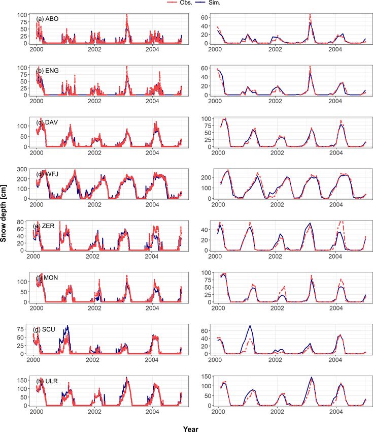
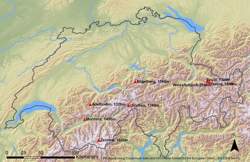
2910                                   F. Willibald et al.: Anthropogenic climate change versus internal climate variability

ture snowpack in the Swiss and French Alps, respectively,          large ensemble has not yet been used to drive a snowpack
and found a significant reduction under all scenarios and          model for regional impact studies.
for all elevation zones. Ishida et al. (2019) and Khadka et           While it is important to estimate the contribution of ICV
al. (2014) found that climate change will lead to severe shifts    to uncertainties in future snow trends, it is just as important
in snow regimes in California and Nepal, respectively.             to investigate the interannual variability (IAV) of snow itself,
   However, the potential impacts of climate change on snow        which is defined as the year-to-year deviation from a long-
hydrology remain disputed, largely because of uncertainties        term mean (He and Li, 2018) and which is likely to change
attributed to future greenhouse gas emissions, model uncer-        under a future climate (IPCC, 2013). While the response of
tainties and internal climate variability (ICV; Beniston et al.,   IAV of snow depths to anthropogenic climate change can
2018). ICV is defined as the natural fluctuations in the cli-      pose risks and increasing uncertainties for agriculture, power
mate system that arise in the absence of any radiative forcing     generation and winter tourism, these processes are only in-
(Hawkins and Sutton, 2009). Typically, studies compare dif-        adequately studied. Again, by complementing multimodel-
ferent emission scenarios to tackle the uncertainties related      based approaches and by separating ICV from forced re-
to future greenhouse gas emissions and use a multimodel en-        sponses, a single-model large ensemble can help answer how
semble approach to estimate uncertainties related to model         interannual variability might respond to changes in climatic
uncertainties (Frei et al., 2018; Marty et al., 2017). While fu-   forcing.
ture greenhouse gas emissions and model uncertainties are             We state the following hypotheses and aim to answering
the subject of multiple studies (Kudo et al., 2017), only very     two research questions: first, ICV is a major source of un-
few studies investigate the impact of ICV on snow (Fyfe et         certainty in trends of future Alpine snow depth. Our research
al., 2017).                                                        question is as follows: what are the uncertainties in future
   When using a multimodel ensemble approach, it is diffi-         trends in Alpine snow depth attributed to ICV? Second, IAV
cult to quantify ICV impacts or separate contributions from        of snow depth will change with anthropogenic climate forc-
ICV and external forcing since it is very challenging to dis-      ing. Hence, our research question is as follows: how does
tinguish between model uncertainties and ICV. The reason           IAV of snow depth change with anthropogenic climate forc-
for this is that intermodel spread is commonly derived from        ing?
the complex coupling of different model structures, param-            To answer these questions, we use a dynamically down-
eterizations and atmospheric initial conditions (Gu et al.,        scaled single-model large ensemble to drive a state-of-the-
2019). Nevertheless, a few studies estimated the fraction of       art, physically based snowpack model for eight stations
uncertainty in the hydrometeorological process chain rang-         across the Swiss Alps. In the first part, we assess the en-
ing from different emission scenarios to the applied impact        semble mean change of snow depths in a future climate. In
model and found that on shorter timescales, ICV represents         the second part, we assess the probabilities for a significant
the single most important source of uncertainty (Fatichi et        reduction in annual mean and maximum snow depth in the
al., 2014; Lafaysse et al., 2014). To investigate the com-         presence of ICV. In the third part, we quantify how inter-
bined influences of ICV and anthropogenic forcing (atmo-           annual variability of snow depth might change in a future
spheric concentration of greenhouse gases and aerosols),           climate.
single-model large ensembles, generated by small differ-
ences in the models’ initial conditions, have been devel-
oped (Deser et al., 2012; Kay et al., 2015; Leduc et al.,          2     Methods and data
2019). Those studies allow a probabilistic assessment of ICV.
Deser et al. (2012), for example, used a 40-member initial-        2.1    Case studies
condition ensemble to estimate the contribution of ICV in fu-
ture North American climate, and Fischer et al. (2013) used a      This study assesses the interdependencies between ICV
21-member single-model ensemble to assess the role of ICV          and anthropogenic climate change for eight stations across
in future climate extremes. Mankin and Diffenbaugh (2014)          the Swiss Alps. The choice of these case studies was
investigated the influence of precipitation variability on near-   driven by the availability of long-term observations needed
term Northern Hemisphere snow trends. Because of high              for model validation and bias correction. The selected
computational costs, those ensembles are usually used on           stations are considered representative as they spread over
the scale of general circulation models; dynamically down-         the whole ridge of the Swiss Alps and cover the northern
scaled single-model large ensembles, using a regional cli-         and southern parts of the mountain range as well as cover
mate model (RCM), are very rare. To our knowledge, only            elevations between 1060 and 2540 m a.s.l. (Fig. 1, Table 1).
Fyfe et al. (2017) used snow water equivalent from a down-         Observational data of temperature, precipitation, wind
scaled single-model large ensemble to estimate the impact of       speed, humidity and incoming shortwave radiation were
ICV on near-term snowpack loss over the United States. Nev-        provided by the Swiss Federal Office of Meteorology and
ertheless, the combined effects of ICV and external forcing        Climatology (MeteoSwiss: https://www.meteoswiss.admin.
on snow remain insufficiently quantified, and a single-model       ch/home/services-and-publications/beratung-und-service/

The Cryosphere, 14, 2909–2924, 2020                                                      https://doi.org/10.5194/tc-14-2909-2020
F. Willibald et al.: Anthropogenic climate change versus internal climate variability                                         2911

Table 1. Summary of case studies.                                 undercatch-corrected by applying a method developed by
                                                                  Hamon (1973), using a function of wind speed and tempera-
      Station         ID            Coordinates     Elevation     ture.
                              (lat ◦ N, long ◦ E)    (m a.s.l.)      Soil layers are not included in our model setup. There-
      Adelboden       ABO             46.5, 7.6          1325     fore, ground surface temperature is determined as a Dirichlet
      Engelberg       ENG             46.8, 8.4          1060     boundary condition (Schmucki et al., 2014) and soil temper-
      Davos           DAV             46.8, 9.9          1560     ature is fixed at 0 ◦ C. To account for site-specific character-
      Montana         MON             46.3, 7.5          1590     istics, we calibrated roughness length and rainfall–snowfall
      Scuol           SCU            46.8, 10.3          1298     threshold temperature. For roughness length, we used val-
      Ulrichen        ULR             46.5, 8.3          1366     ues between 0.01 and 0.08. For rainfall–snowfall discrim-
      Weissfluhjoch   WFJ             46.8, 9.8          2540     ination, we used threshold temperatures between 0.2 and
      Zermatt         ZER             46.0, 7.8          1600     1.2 ◦ C, which lies well within the calibration ranges between
                                                                  −0.4 and 2.4 ◦ C based on results from Jennings et al. (2018).
                                                                  The calibration was carried out individually for each site. A
datenportal-fuer-lehre-und-forschung.html, last access:           threshold of 50 % in relative humidity was set for all stations
18 August 2020) and the WSL Institute of Snow and                 for rainfall–snowfall discrimination.
Avalanche Research (SLF) in a 3-hourly temporal resolu-              SNOWPACK usually operates on very high temporal reso-
tion. Daily measurements of snow depth used for model             lutions. After an initial sensitivity analysis, to get better sim-
validation stem from the same sources. The temporal               ulation results, the meteorological input was resampled to an
coverage of the observational data for the purpose of bias        hourly resolution in order to run at hourly time steps. Precip-
correction and model validation ranges from 1983 to 2010.         itation was evenly disaggregated from a 3-hourly time step
                                                                  to 1 h, while the remaining parameters were linearly interpo-
2.2   The SNOWPACK model                                          lated. The meteorological parametrizations and the temporal
                                                                  resampling were performed by the MeteoIO library (version
SNOWPACK is a physically based, one-dimensional snow              2.8.0) embedded within Snowpack (version 3.5.0). The case
cover model (Lehning et al., 1999). It was originally de-         studies were validated based on observed daily and monthly
veloped for avalanche forecasting (Lehning et al., 2002a)         snow depths.
but is increasingly used for climate change studies (Kat-
suyama et al., 2017; Schmucki et al., 2015). SNOWPACK is          2.3   Simulation data
highly advanced with regard to snow microstructural detail.
The model uses a Lagrangian finite-element method to solve        In this study, we use climate model data from a new single-
the partial differential equations regulating the mass, en-       model large ensemble, hereafter referred to as the ClimEx
ergy and momentum transport within the snowpack. Calcu-           large ensemble (ClimEx LE; Leduc et al., 2019; von Trentini
lations of the energy balance, mass balance, phase changes,       et al., 2019), to analyze the combined influence of ICV and
water movement and snow transport by wind are included            climate change on future snow depth. The ClimEx LE con-
in the model. Finite elements can be added through solid          sists of 50 members of the Canadian Earth System Model
precipitation and subtracted by erosion, melt water runoff,       (CanESM2; Arora et al., 2011), which is downscaled for
evaporation or sublimation (Lehning et al., 1999, 2002a, b;       a European and North American domain by the Canadian
Schmucki et al., 2014). Usual temporal resolutions range          Regional Climate Model (CRCM5; Šeparović et al., 2013).
from 15 min (e.g., for avalanche forecasting) to 1 h (e.g.        Each ensemble member undergoes the same external forc-
for long-term climate studies and spatially distributed sim-      ing and starts with identical initial conditions in the ocean,
ulations). Minimum meteorological input for SNOWPACK              land and sea-ice model components but slightly different ini-
is air temperature, relative humidity, incoming or reflected      tial conditions in the atmospheric model. The 50 members
shortwave radiation, incoming longwave radiation or surface       of the CanESM2 originate from five families of simulations,
temperature, wind speed, and precipitation. Due to the lack       each starting at different 50-year intervals of a preindus-
of measurements, incoming longwave radiation had to be es-        trial run with a stationary climate and ranging from 1850 to
timated based on air temperature, incoming shortwave radi-        1950. In 1950, small differences in the initial conditions are
ation and relative humidity; using the parameterization by        used to separate each family into 10 members. After apply-
Konzelmann et al. (1994), Shakoor et al. (2018) and Shakoor       ing small atmospheric perturbations in the initial conditions,
and Ejaz (2019) applied this method for multiple sites and el-    each member evolves chaotically over time. Therefore, the
evations and found that it gives reliable estimates. As wind-     model spread shows how much the climate can vary as a re-
induced gauge undercatch underestimates precipitation, es-        sult of random internal variations (Deser et al., 2012). This
pecially for mixed and solid precipitation, we do not use         makes all 50 members equally likely, plausible realizations
the original measured precipitation data to run the model.        of climate change over the next century. Until 2005 the en-
As described in Schmucki et al. (2014), precipitation was         semble is driven by observed forcing; from 2006 to 2099 all

https://doi.org/10.5194/tc-14-2909-2020                                                 The Cryosphere, 14, 2909–2924, 2020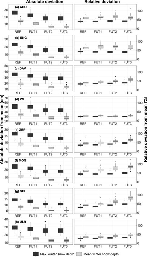
2912                                   F. Willibald et al.: Anthropogenic climate change versus internal climate variability

Figure 1. Overview map of case studies used for this study (produced using Copernicus data and information funded by the European Union
EU-DEM layers).

simulations are forced with concentrations according to the           models still have a systematic model bias and as our im-
RCP8.5 scenario (Moss et al., 2010).                                  pact model simulates snow for a particular one-dimensional
   The 50 members are then dynamically downscaled over                point in space, another downscaling or bias adjustment step
Europe using CRCM5 with a horizontal grid size of 0.11◦ on            is needed to adjust systematic model biases and to bridge
a rotated latitude–longitude grid, corresponding to a 12 km           the gap between RCM simulations and the impact model.
resolution (von Trentini et al., 2019). Detailed information          There exist multiple methods for bias adjustment and down-
on the design of the experiment can be found in Leduc et              scaling, and approaches are dependent on the study purpose.
al. (2019). The ClimEx LE provides meteorological data at a           While, for example, the delta change approach is robust and
3-hourly temporal resolution.                                         easy to implement, the method neglects potential changes in
   In an intercomparison experiment by von Trentini et                variability and is therefore not suitable for our study. In re-
al. (2019), the ClimEx LE was compared to 22 members                  cent years, many studies have concluded that quantile map-
of the EURO-CORDEX multimodel ensemble. It was found                  ping (QM) performs similar or superior to other statistical
that the ClimEx LE shows stronger climate change signals,             downscaling approaches (Feigenwinter et al., 2018; Gutiér-
and the single-model spread is usually smaller compared to            rez et al., 2019; Ivanov and Kotlarski, 2017).
the multimodel ensemble spread. Our analysis and Leduc et                When multimodel ensembles are bias-corrected, usually
al. (2019) found a substantial bias between the ClimEx LE             each simulation is corrected separately, whereas bias adjust-
and observational data aggregated to the 12 km grid. Espe-            ing a single-model large ensemble requires specific consid-
cially over the Alps, a strong wet bias was identified. With          erations as the chosen method should not only correct the
regard to temperature, we found a cold bias for most grid             bias of each individual member but should also retain the in-
points covering the Swiss Alps. The bias between model data           dividual intermember variability (Chen et al., 2019). We ap-
and observations justifies the application of a bias adjustment       plied a distribution-based quantile mapping approach to bias-
procedure, which is explained in Sect. 2.4.                           correct and downscale the model data to the station scale in
                                                                      one step, based on the daily translation method by Mpela-
2.4    Bias adjustment                                                soka and Chiew (2009). Several studies tested this method
                                                                      and confirmed a reasonable performance (Gu et al., 2019;
As simulations from general circulation models are usually            Teutschbein and Seibert, 2012). A downscaling-to-station
too coarse to be directly used as input in impact models,             approach was also performed for the official CH2018 Swiss
CanESM2 was dynamically downscaled to a 12 km resolu-                 climate scenarios (Feigenwinter et al., 2018). We modified
tion, which better represents regional topography and there-          the approach in the form that it was applied to a transient cli-
fore regional climatology. As practically all regional climate        mate simulation ranging from 1980 to 2099, and, in contrast

The Cryosphere, 14, 2909–2924, 2020                                                       https://doi.org/10.5194/tc-14-2909-2020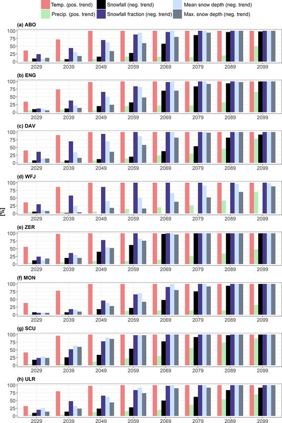
F. Willibald et al.: Anthropogenic climate change versus internal climate variability 2913
to previous studies that use daily scaling factors, it is based for exactly this period. Due to this reason and as the per-
on subdaily scaling factors. The last-mentioned modification formance of the chosen bias correction method is already
was necessary as SNOWPACK needs subdaily meteorologi- the subject of the studies by Chen et al. (2019) and Gu et
cal input. al. (2019), we do not present the validation exercise in detail.
In a first step, we computed the empirical distributions Instead we focus on a validation that is highly relevant for
of observed and simulated climate variables for the baseline snow accumulation, namely on the performance of the bias
period 1984 to 2009. We chose this period as it is the pe- adjustment with regard to the snowfall fraction assuming the
riod during which all of the stations have the smallest count calibrated SNOWPACK rain–snow temperature thresholds.
of missing data. Overall, 99 quantiles were estimated sepa- This is of special interest as a univariate bias adjustment ap-
rately for each month and each 3-hourly time step of the day. proach, as employed here, does not explicitly correct for bi-
The grid cells overlying the respective climate stations de- ased intervariable dependencies, which could, among other
scribed in Sect. 2.1 provide the simulated input series. For things, affect the snowfall fraction.
the ClimEx LE simulations, all 50 members were aggregated SNOWPACK itself was calibrated for the period 1985
to compute a single empirical distribution. A large part of to 1989 and cross-validated for different 5-year periods be-
the internal variability would be removed or filtered if the tween 1990 and 2009 using observed meteorological input,
distributions were calculated independently for each mem- which was compared to measured snow depths. All periods
ber (Chen et al., 2019). Thus, we computed the distribution provide similar results. For a clearer visualization, we only
based on the pooled ensemble members because all runs are show results for the period 2000 to 2004. To assess good-
derived from the same climate model with the same forcing ness of fit, we compared daily and monthly measured snow
and are therefore assumed to have the same climatological heights with modeled snow heights simulated with observed
bias (Chen et al., 2019; Gu et al., 2019). meteorological input using several performance indicators
In a second step, we computed scaling factors between the such as mean absolute error (MAE), Nash–Sutcliffe effi-
simulated and observed data in the baseline period. For tem- ciency (NSE) coefficient, coefficient of determination (R 2 )
perature, an additive scaling factor was estimated, while for and index of agreement (d; e.g., Krause et al., 2005; Legates
the remaining variables multiplicative scaling factors were and McCabe, 1999).
estimated. In a last step, for temperature the scaling factors
were added to the empirical distributions of each single en- 2.6 Statistical analysis of simulated snow depth
semble member, while for the remaining variables the scal-
ing factors were multiplied with the empirical distributions In the first part of our analysis, we estimate the ensemble
of the simulations. The same scaling factors were transiently mean changes for annual mean and maximum snow depth be-
applied to the distribution functions of 25-year slices of each tween the reference period ranging from 1980 to 2009 (REF)
ensemble member. and three future periods ranging from 2010 to 2039 (near fu-
The method does not take into account intervariable de- ture: FUT1), 2040 to 2069 (midfuture: FUT2) and 2070 to
pendency. As SNOWPACK is a physically based model, 2099 (far future: FUT3).
physical inconsistencies in the data can lead to serious model In the second part of the analysis, we estimate the uncer-
errors. For example, precipitation occurring simultaneously tainties in future snow trends (and their drivers) emerging
with low humidity will result in model error. As we use a from ICV.
univariate bias adjustment approach, we also had to test the We apply the Mann–Kendall (MK) trend detection test
results for these inconsistencies. (Kendall, 1975; Mann, 1945) to test for statistically signif-
icant trends of different lengths of time series starting in the
2.5 Validation of bias adjustment and SNOWPACK year 2000 and ending between 2029 and 2099. The Mann–
Kendall test is frequently used in climatological and hydro-
The performance of the applied bias adjustment approach as logical applications (Gocic and Trajkovic, 2013; Kaushik et
well as the performance of SNOWPACK and the snow simu- al., 2020). The MK test statistic (S) is computed as
lations using the ClimEx LE as a driver were validated prior
n−1 X
n
to continued analyses. X
S= sgn(xj − xi ), (1)
To evaluate the performance of the bias adjustment ap-
i=1 j =i+1
proach, we compared the statistical characteristics of ob-
served meteorological variables to the bias-adjusted ClimEx where xi and xj are the data points at times i and j ; n rep-
LE for subdaily, daily, monthly and yearly values and com- resents the length of the time series; sgn(xj − xi ) is a sign
pared the diurnal and annual regimes of the corrected param- function defined as
eters. We obtained good results in the calibration period 1984
to 2009.
+1, if xj − xi > 0
In terms of distributional quantities and climatologies, this sgn xj − xi = 0, if xj − xi = 0 (2)
is to be expected as the bias correction scheme was calibrated
−1, if xj − xi < 0.
https://doi.org/10.5194/tc-14-2909-2020 The Cryosphere, 14, 2909–2924, 2020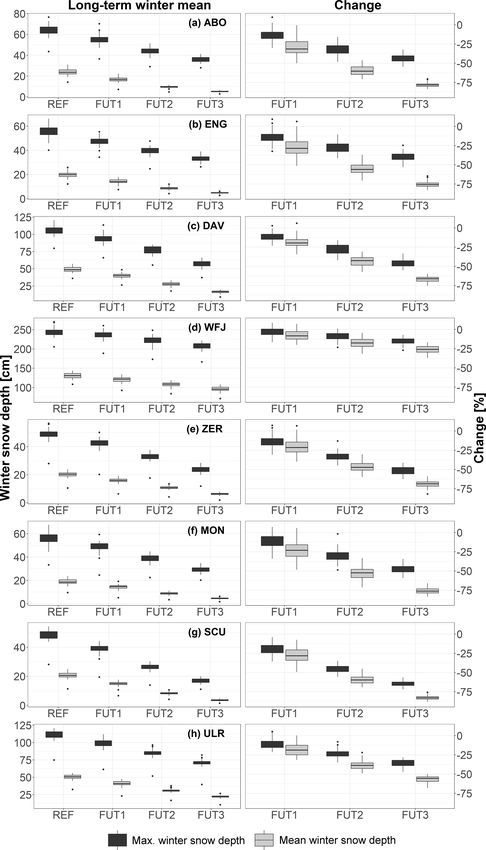
2914                                  F. Willibald et al.: Anthropogenic climate change versus internal climate variability

   The null hypothesis of the MK test is that a time series has
no trend (Libiseller and Grimvall, 2002). In this study, trend
significance was tested for p values of 0.01, 0.05 and 0.1. As
air temperature below a certain threshold occurring simulta-
neously with precipitation is the most important prerequisite
of snowfall (Morán-Tejeda et al., 2013; Sospedra-Alfonso et
al., 2015), we do not only test for future snow depth trends
but also for the drivers of future snow conditions. For that
reason, we also apply the Mann–Kendall test to temperature,
precipitation, snowfall fraction and snowfall time series.
   In the third part of the study, we estimate the change in
IAV. As a measure for IAV, we use the standard deviations
of annual mean and maximum snow depths for the respec-
tive reference and future periods. The standard deviation is
commonly used as a measure of IAV, such as in Siam and
Eltahir (2017). All analyses were performed with the statisti-
cal software R (R Core Team, 2017). All analyses in Sect. 3.3
to 3.5 are performed for mean and maximum winter snow
depths. Winter is defined as the months November to April.

3     Results

3.1    Validation of SNOWPACK

The validation results of SNOWPACK using meteorological           Figure 2. Validation results of SNOWPACK. Simulated daily (left)
observations as input are summarized in Fig. 2. From Table 2,     and monthly (right) mean snow depth driven by 3-hourly meteo-
we can deduce a good model fit. For all stations, the annual      rological observations (sim) vs. measured daily and monthly mean
snow regime is very similar between observations and sim-         snow depth (obs) for the period 2000 to 2004. See Table 1 for the
                                                                  abbreviations of case studies.
ulations, and the month of maximum snow depth is always
identical. Maxima are also well represented. There is no sys-
tematic over- or underestimation visible across stations. Only
for the station Montana is a systematic overestimation of sim-       Figure 3 visualizes the mean winter snowfall fraction for
ulated snow depths across all years apparent.                     each station based on observed temperature and precipita-
   The performance indicators of daily measured and simu-         tion and based on the bias-adjusted temperature and precip-
lated snow depths show good results for all stations. With        itation data for the corresponding rainfall–snowfall thresh-
an R 2 and NSE larger than 0.75 and an index of agreement         old temperatures. Snowfall fractions based on observations
larger than 0.9, the stations Davos, Montana, Zermatt, Ul-        and bias-adjusted simulations are almost similar for Adel-
richen and Weissfluhjoch show a very good model perfor-           boden, Engelberg, Davos and Weissfluhjoch. For Scuol, the
mance. The low-elevation stations Engelberg and Adelboden         bias-adjusted ClimEx LE underestimates the observed snow-
as well as Scuol still show a reasonably good model fit with      fall fraction by 12 % and for Ulrichen by up to 20 %. For the
an R 2 larger or equal to 0.6 and an NSE larger than 0.5 as       two stations Zermatt and Montana, we find an even stronger
well as an index of agreement (d) larger than 0.85.               underestimation of 33 % and 50 %, respectively. The results
                                                                  imply that there is no systematic error between observed and
3.2    Performance of bias adjustment and ensemble                simulated snowfall fractions, but there are stations that show
       SNOWPACK simulations                                       a significant underestimation of snowfall fraction compared
                                                                  to observations. The potential reasons for this underestima-
Intervariable dependence between precipitation and humid-         tion are addressed in the discussion (Sect. 4).
ity as well as incoming shortwave radiation was not cor-             In Fig. 4 we show the long-term monthly mean snow
rupted through the bias correction (e.g., there were no cases     depths for observations, simulations driven by observed
of precipitation and simultaneously low humidity or precip-       meteorological input and simulations driven by the bias-
itation and simultaneously high incoming shortwave radia-         adjusted ClimEx LE. As already mentioned in Sect. 3.1, the
tion; not shown). We concentrate the presentation of our re-      comparison between observations and SNOWPACK simula-
sults on the impacts of bias adjustment on temperature and        tions driven by observational data shows a good model fit for
precipitation dependencies and consequently snowfall frac-        all stations. For the stations Adelboden, Engelberg, Davos,
tion as this is an essential part of the snow modeling process.   Weissfluhjoch and Scuol, the 50 ClimEx LE simulations en-

The Cryosphere, 14, 2909–2924, 2020                                                   https://doi.org/10.5194/tc-14-2909-2020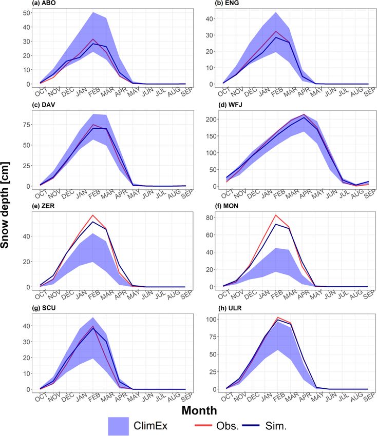
F. Willibald et al.: Anthropogenic climate change versus internal climate variability                                                      2915

Table 2. Goodness-of-fit measures between measured daily snow depth and SNOWPACK simulated daily snow depth driven by 3-hourly
meteorological observations for the period 2000 to 2004. Measures are mean absolute error (MAE), Nash–Sutcliffe coefficiency (NSE),
coefficient of determination (R 2 ) and index of agreement (d). See Table 1 for the abbreviations of case studies.

                                           ABO      ENG      DAV        WFJ       ZER       MON    SCU     ULR
                                  MAE       3.91     5.75    4.47       18.5         4.58   5.66   4.49    7.21
                                  NSE       0.59     0.64    0.92       0.91         0.79   0.86   0.51    0.88
                                  d         0.87      0.9    0.98       0.98         0.94   0.96    0.9    0.97
                                  R2         0.6     0.66    0.92       0.91         0.79   0.87   0.75     0.9

Figure 3. Mean winter snowfall fraction based on observations
(obs; red) and for the bias-adjusted ClimEx LE (blue) for the pe-
riod 1984 to 2009. temp-th indicates the calibrated snowfall–rainfall
separation threshold for the respective station. See Table 1 for the
abbreviations of case studies.

close the observed snow depths for the calibration period of
the bias adjustment. This implies a good performance of the
bias adjustment. As shown above, the bias-adjusted data set
systematically underestimates snowfall fraction in Zermatt                     Figure 4. Long-term monthly mean snow depth for observations
and Montana, resulting in a pronounced underestimation of                      (obs), simulations driven by meteorological observations (sim) and
simulated snow depths. The two stations are not excluded                       the ensemble spread of simulations driven by the ClimEx LE for
from further analyses, but we have to clarify that those results               the period 1984 to 2009. See Table 1 for the abbreviations of case
must be interpreted cautiously and that we cannot consider                     studies.
absolute snowfall fraction or snow depth values for those sta-
tions.
   Lastly, it is important to validate the ability of the ClimEx               3.3     Mean climate change signal
LE SNOWPACK simulations to reproduce IAV. In Fig. 5, we
                                                                               Both the impacts of ICV on future snow trends and the
present IAV of winter mean snow depth for the ClimEx LE
                                                                               changes in IAV under a given emission scenario must be put
SNOWPACK simulations, observed snow depth and simu-
                                                                               into perspective to the ensemble mean climate change sig-
lated snow depths based on observed meteorological input.
                                                                               nal. To do so, we present the absolute and relative changes
For all stations but Adelboden, Zermatt and Montana, IAV of
                                                                               in mean and maximum winter snow depth between our ref-
simulations driven by observational data lies within the enve-
                                                                               erence and future periods. Figure 6 visualizes the mean and
lope of the 50 ClimEx LE members. For the stations Zermatt
                                                                               maximum winter snow depths for the reference and future
and Montana, the systematic underestimation of snow depth
                                                                               periods and the respective percentage change. For the ensem-
consequently leads to an underestimation of IAV.
                                                                               ble mean, we find a continuous and significant decrease in
                                                                               mean and maximum snow depth over all stations. While ab-
                                                                               solute changes are partly stronger for maximum winter snow

https://doi.org/10.5194/tc-14-2909-2020                                                              The Cryosphere, 14, 2909–2924, 2020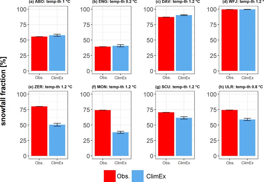
2916 F. Willibald et al.: Anthropogenic climate change versus internal climate variability
Figure 5. Interannual variability of mean winter snow depth for
SNOWPACK simulations using ClimEx LE as a driver, using ob-
served meteorological data as a driver (sim) and observed IAV (obs)
of mean winter snow depth for the period 1984 to 2009. The boxes
represent the interquartile range with the median as a horizontal
line. The whiskers represent 1.5 times the interquartile range, and
the dots represent outliers. See Table 1 for the abbreviations of case
studies.
depths, the percentage decrease in mean winter snow depth
is more severe for all case studies, because of the large dif-
ferences in the absolute values of mean and maximum snow
depth. All stations below 2000 m a.s.l. except Ulrichen show
a similarly strong decrease in mean winter snow depth. The
decrease in the near-future period is relatively small, and for
all stations but Scuol, there is at least one member that sim-
ulates a small increase in winter mean and maximum snow
depth. For the mid- and far-future periods, decreases range
from −30 % to −70 % until 2069 and up to −60 % to −80 %
until 2099. For Ulrichen, we obtain a slightly smaller de-
crease of up to −60 % until 2099. For the high-elevation sta-
tion Weissfluhjoch, decreases are considerably lower, rang-
ing from −20 % until 2069 to −25 % until 2099. The per-
centage decreases for maximum snow depths are consider-
ably lower compared to those for mean snow depths, with
an ensemble mean ranging from −25 % to −40 % until 2069 Figure 6. Winter mean maximum and mean snow depth (cm; left)
and −30 % to −60 % until 2099 for all stations but Weiss- for the ClimEx LE and mean changes (%; right) between the REF
fluhjoch. For Weissfluhjoch we observe ensemble mean de- period 1980 to 2009 and FUT1 (2010 to 2039), FUT2 (2040 to
creases of −10 % until 2069 and −15 % until 2099. In the 2069) and FUT3 (2070 to 2099) for the stations Adelboden (ABO),
discussion, we compare these values to results from other Engelberg (ENG), Davos (DAV), Weissfluhjoch (WFJ), Zermatt
(ZER), Montana (MON), Scuol (SCU) and Ulrichen (ULR). The
studies.
boxes represent the interquartile range with the median as a hori-
zontal line. The whiskers represent 1.5 times the interquartile range,
3.4 Significance of future snow depth trends
and the dots represent outliers.
Despite the strong mean climate change signal described in
Sect. 3.3, Sect. 3.4 points out the important role of ICV for
the detection of statistically significant trends in future time test for a positive trend in winter mean temperature and win-
series of snow depth and its most important drivers tempera- ter precipitation sums and a negative trend for winter snow-
ture, precipitation, snowfall fraction and snowfall. Note that, fall fraction and snowfall as well as winter mean and maxi-
according to the poor validation results, we cannot draw con- mum snow depth for the lowest station, Engelberg, and the
clusions on the absolute values of snowfall fraction, snowfall highest station, Weissfluhjoch, for 1 %, 5 % and 10 % signifi-
and snow depth for the stations Zermatt and Montana. Nev- cance levels. Each time series starts in the year 2000 and ends
ertheless, we can apply the trend test and compare relative in 5-year intervals between 2029 and 2099. Figure 8 shows
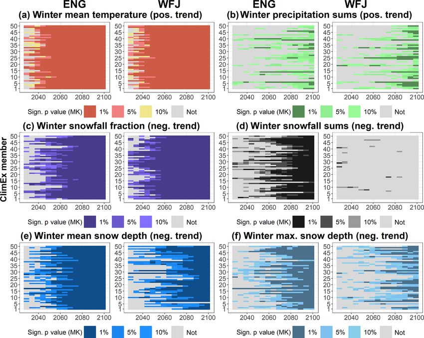
changes. Figure 7 visualizes the results of the Mann–Kendall the percentage of members with a significant Mann–Kendall
The Cryosphere, 14, 2909–2924, 2020 https://doi.org/10.5194/tc-14-2909-2020F. Willibald et al.: Anthropogenic climate change versus internal climate variability 2917
test result for all case studies based on the 5 % significance Similar to snowfall fraction, we find a steady increase in
level. the count of members with a statistically significant negative
With regard to temperature, all case studies show a rapidly trend in winter mean snow depth, but compared to winter
increasing percentage of significant positive trends. For a temperature, this development starts considerably later. Gen-
30-year period, already between 30 % and 60 % of mem- erally, the trend significance is stronger compared to snow-
bers show significant results. Until the year 2049 more than fall fraction, but there is still a 50 % to 30 % chance (for all
90 % of members show a significant positive trend, and by stations but Scuol, where more than 80 % of members show
2059 all stations show a 100 % trend significance. Here we significant negative trends) that ICV will superimpose an-
can clearly conclude that the anthropogenic climate change thropogenic climate change impacts on mean winter snow
signal is significantly stronger than the ICV of temperature, depth over a period of 50 years. By 2069, the percentage
i.e., the forced trend emerges from internal climate variabil- of significant members increases to more than 90 %. The
ity. For precipitation, we find a completely different picture. stronger significance of mean snow depth compared to snow-
For all stations but Scuol, there is no clear sign towards an fall fraction and the higher significance compared to snowfall
increase in future winter precipitation sums. There is a ten- sums imply the combined effects of a very uncertain decrease
dency towards an increasing number of members with a sig- in snowfall sums combined with more rapid and more fre-
nificant positive trend in precipitation towards the end of the quent snow melt. Lastly, maximum winter snow depth shows
century, but the percentage is below 50 % for all stations but a significantly different evolution than mean winter snow
Scuol until 2089. For Scuol, there is a clear sign towards an depth. Here, we also obtain large differences between the
increase in winter precipitation sums. Here, more than 75 % lower-lying stations and the highest station, Weissfluhjoch.
of members show a significant positive trend in winter pre- For most stations but Scuol, there is a probability of more
cipitation sums. In summary, we cannot detect a clear climate than 50 % of no significant negative trend in future maxi-
change signal for precipitation because of strong ICV. mum snow depth over a period of 50 years. For Scuol this
With regard to snowfall fraction, we find a consistent in- probability is only 15 %, while it is 80 % for Weissfluhjoch.
crease in members with a significant negative trend in snow- Over a period of 80 years all stations but Weissfluhjoch show
fall fraction over time, but, as expected, the strong tempera- a significant decrease in maximum snow depths in more than
ture signal does not translate into a similarly strong trend sig- 90 % of the cases. For Weissfluhjoch a high probability for
nificance, and there are significant differences between case ICV to superimpose anthropogenic climate change remains.
studies. Over a 50-year period, most stations show signifi- By 2049 the percentage of negative trends is below 20 %, by
cance for only up to 70 % of members. The stations Davos, 2079 the probability is still below 50 %, and even over a pe-
Weissfluhjoch and Scuol, the stations with the highest snow- riod of 100 years there is a 20 % chance of no significantly
fall fraction in the reference period (besides Scuol), show sig- negative trend in maximum winter snow depth. This empha-
nificant reductions for 75 % to 90 % of members over this pe- sizes that also in the far future, individual important snow
riod. This emphasizes the huge contribution of ICV to future peaks can be expected, especially at high elevations.
trends in winter snowfall. Over a period of 60 years, there Our results underline the outstanding contribution of ICV
is still a 30 % chance of not detecting a significant negative to uncertainties related to future trends in snow depth and its
trend in snowfall fraction for Montana due to ICV, but by drivers. Especially in the near-future, ICV can hamper a clear
2069 all stations show significant decreases in snowfall frac- impact signal of anthropogenic warming as the strong signal
tion for more than 90 % of members. for mean winter temperature does not directly translate into
In contrast to snowfall fraction, we find a lower statisti- clear snow-related signals.
cal significance for negative trends of total winter snowfall
sums. For all stations except Weissfluhjoch, over a period 3.5 Changes in interannual variability
of 60 years, the percentage of statistically significant nega-
tive trends in winter snowfall sums is only between 25 % and In Sect. 3.4 we revealed the large contribution of ICV to un-
60 %. Over a period of 80 years between 60 % and 90 % of certainties related to future trends in snow depth. However,
members show a statistically negative trend, and by the end the variability of snow depth itself is likely to change with an-
of the century only the stations Engelberg, Zermatt, Montana thropogenic forcing. Here we investigate how IAV of mean
and Scuol show a trend significance for 100 % of members. and maximum snow depth, defined as the standard deviation
For the station Weissfluhjoch, no statistically significant neg- of snow depth over a period of 30 years, is likely to change
ative trend is obtained over any period. Even over 100 years under RCP8.5. From Figs. 6 and 9 we can see that a grad-
none of the members show a significant reduction in winter ual decrease in winter mean and maximum snow depth is
snowfall sums. These results imply that, despite the strong accompanied by a decrease in absolute IAV. Nevertheless, in
temperature increase and a significant reduction in snowfall relative terms (relative to the mean of the corresponding pe-
fraction, a reduction in total snowfall sums at this site re- riods), IAV can strongly increase in the future, but there are
mains very uncertain. differences between mean and maximum snow depth and at
different stations. In the reference period and at lower ele-
https://doi.org/10.5194/tc-14-2909-2020 The Cryosphere, 14, 2909–2924, 20202918 F. Willibald et al.: Anthropogenic climate change versus internal climate variability
Figure 7. Heat maps of trend significance for the Mann–Kendall test for different periods starting in 2000 and ending between 2029 and
2099 for winter mean temperature, winter precipitation sums, winter snowfall fraction, winter snowfall sums, and winter mean and maximum
snow depth for the lowest station, Engelberg (ENG), and the highest station, Weissfluhjoch (WFJ).
vation, relative IAV of mean snow depth lies between 40 % 4 Discussion
(Scuol) and 60 % (Engelberg), and relative IAV of maximum
snow depth lies between 20 % (Scuol) and 60 % (Engelberg). Many studies have significantly improved our knowledge
For most cases, relative IAV of mean snow depth is larger about the cryosphere in a future climate (Barnett et al., 2005;
compared to maximum snow depth. For Weissfluhjoch the Beniston et al., 2018). Nevertheless, the predominant num-
overall variability is lower compared to the other stations ber of studies focuses on changes in the mean, while studies
(25 % in the reference period), and maximum snow depth on the interdependencies of climate change and ICV are very
has a larger variability than mean snow depth. For Weiss- rare. Our analysis is the first study that uses a single-model
fluhjoch, an increase in relative IAV can be found for neither large ensemble as input for a physically based snow model.
mean nor maximum snow depth. In contrast, an increase in This allows a probabilistic uncertainty assessment of future
relative IAV for the stations Adelboden, Engelberg, Davos, snow trends in the European Alps attributable to ICV. We
Zermatt, Montana, Scuol and Ulrichen is projected. Larger further estimate how IAV might change in a future climate.
increases in relative IAV are obtained for mean winter snow
depth, while the increases for maximum snow depth are very 4.1 Uncertainties and limitations
small. For Davos, for example, we find an ensemble mean
increase in relative IAV of mean snow depth from 40 % to While we are gaining important insights into the dynamics
60 % until the end of the century. Increases in relative IAV of mean, maximum and interannual variability of snow depth
of maximum snow depth range from 35 % to 40 %. For Mon- and the role of ICV under climate change conditions, a num-
tana IAV increases from 60 % in the reference period to more ber of important uncertainties and limitations must be taken
than 90 % in the future 2 period. For Scuol we find an in- into account, which span over the whole modeling process.
crease from 40 % up to 80 % between the two periods. Important boundary conditions are that our results are highly
dependent on the choice of the emission scenario and the
combination of global climate model (GCM) and RCM as
well as the selected bias adjustment approach. First, it must
be stated that the ClimEx LE is still unique regarding mem-
The Cryosphere, 14, 2909–2924, 2020 https://doi.org/10.5194/tc-14-2909-2020F. Willibald et al.: Anthropogenic climate change versus internal climate variability 2919
Figure 8. Percentage of significant trends (p value of 5 %) for time
series of temperature, winter precipitation sums, snowfall fraction,
snowfall sums, and mean and maximum snow depth starting in 2000
and ending between 2029 and 2099 for all case studies. See Table 1
for the abbreviations of case studies.
Figure 9. Interannual variability for the REF (1980 to 2009), FUT1
(2010 to 2039), FUT2 (2040 to 2069) and FUT3 (2070 to 2099) pe-
bers and spatiotemporal resolution; like other currently exist- riods expressed as the absolute standard deviation (cm; left) and
ing single-RCM initial-condition large ensembles, it is avail- standard deviation relative to the mean (%; right) for mean and
able under RCP8.5 only. Being aware of the extreme char- maximum snow depth for the stations Adelboden (ABO), Engel-
acter of this greenhouse gas (GHG) concentration scenario berg (ENG), Davos (DAV), Weissfluhjoch (WFJ), Zermatt (ZER),
and the high sensitivity of the GCM–RCM combination, the Montana (MON), Scuol (SCU) and Ulrichen (ULR). The boxes rep-
resent the interquartile range with the median as a horizontal line.
results obtained from the presented analyses are considered
The whiskers represent 1.5 times the interquartile range, and the
valid as they represent the expected dynamics and states of dots represent outliers.
other emission scenarios but reach certain levels of change
earlier in time.
Due to the single-model approach, it is understood that the
presented setup has limited capacity in providing a robust
estimate of anthropogenic climate change; this is where mul- tini et al., 2019). Nevertheless, multimodel ensembles make
timodel ensemble setups have clear advantages (Tebaldi and it very difficult to distinguish between model uncertainties
Knutti, 2007). Comparing the detected climate change sig- and ICV, which is a major advantage of our approach, when
nals of the ClimEx LE with the EURO-CORDEX ensemble the goal is to study ICV. Of course, it would be of interest
shows that the data used for this study provide a highly sen- to estimate model uncertainties and do a probabilistic analy-
sitive forced response, yet within plausible ranges (von Tren- sis of ICV. To do so an ensemble of ensembles would be the
https://doi.org/10.5194/tc-14-2909-2020 The Cryosphere, 14, 2909–2924, 20202920 F. Willibald et al.: Anthropogenic climate change versus internal climate variability
preferred approach. Due to computational limitations, such pendencies between anthropogenic climate change and ICV
analyses are not yet feasible, especially on the regional scale. and its impacts on snow depth in the Alps. Its novelty stems
Another source of uncertainty is the choice of the bias ad- from a true probabilistic assessment of ICV. In the first part of
justment methodology. While quantile mapping was found our results section, we presented the ensemble mean change
to be similar or superior to many other bias adjustment ap- between a reference period (1980 to 2009) and three future
proaches (Gutiérrez et al., 2019; Ivanov and Kotlarski, 2017; periods and found significant decreases in ensemble mean
Teutschbein and Seibert, 2012), it has some important draw- snow depth in the future. Schmucki et al. (2015) present a
backs. QM assumes stationarity of the model bias struc- similar analysis for partly the same case studies using 10
ture, an assumption that is uncertain under changing climatic GCM–RCM model chains from the ENSEMBLES project
conditions (Maraun, 2013). Furthermore, QM cannot cor- under the IPCC A1B emission scenario. Although the refer-
rect misrepresented temporal variability (Addor and Seib- ence periods do not fully match (Schmucki et al., 2015, use
ert, 2014). Therefore, interannual variability was validated 1984 to 2010), we can put the changes between the reference
in Sect. 3.2, yielding acceptable results. When applied in a period and the mid- (2040 to 2069 in this study and 2045 to
downscaling context, QM cannot reproduce local processes 2074 for Schmucki et al., 2015) and far-future period (2070
and feedbacks as QM is a purely empirical approach (Feigen- to 2099) into perspective. For Weissfluhjoch, Schmucki et al.
winter et al., 2018; Kotlarski et al., 2015). In contrast, QM (2015) simulate a mean decrease of 28 % (near future) and
can modify the raw climate change signal and simulated 35 % (far future), which is close to our simulation results of
trends (Ivanov et al., 2018). This point is especially impor- −18 % (near future) and −27 % (far future) in mean winter
tant in our study as we have to correct each member based snow depth and −30 % (near future) and −42 % (far future)
on the empirical distribution of the whole ensemble to re- for annual mean snow depth. Both studies show comparable
tain the internal climate variability. Therefore, the climate decreases in mean snow depth at Weissfluhjoch, although our
change signals of the single members are modified. Can- study uses the much stronger RCP8.5 compared to the A1B
non et al. (2015) developed a method that preserves the raw scenario in Schmucki et al. (2015).
climate change signal, but applied to this study it would In the near and far future, Schmucki et al. (2015) found
only preserve the ensemble mean signal. Further research is an ensemble spread of mean snow depth of 35–135 cm (near
needed to develop potential methods that preserve the climate future) and 30–130 cm (far future), whereas we simulate an
change signal for single members from single-model ensem- ensemble spread of 84–119 cm (near future) and 71–108 cm
bles. As a last point, we employ a univariate bias adjustment (far future) for winter mean snow depth and 48–70 cm (near
approach, which treats all meteorological variables indepen- future) and 39–60 cm (far future) for annual mean snow
dently. While intervariable consistency cannot be guaran- depth.
teed (Feigenwinter et al., 2018), multiple studies show that Marty et al. (2017) use 20 different GCM–RCM chains to
QM generally maintains intervariable consistency (Ivanov compare the impacts of different emission scenarios on mean
and Kotlarski, 2017). In the course of this work, intervariable snow depth for two catchments in Switzerland that partly also
consistency was validated, and we obtained good results for cover stations analyzed in this study. For the Aare catchment
radiation, precipitation and humidity. Variable consistency that covers our stations Adelboden and Engelberg and under
with regard to snowfall fraction was inaccurate for individual IPCC A2, Marty et al. (2017) simulate an ensemble mean de-
case studies. Prior to bias adjustment, a strong cold bias over crease of 65 % and an ensemble spread between −33 % and
most grid points caused snowfall fraction to be significantly −85 % between the reference period (1999 to 2012) and the
too high. Therefore, bias correction generally improved the far future (2070 to 2099). For our case studies Adelboden and
simulated snowfall fractions. The exploration of possible rea- Engelberg, we find decreases in mean snow depth between
sons for inaccurate snowfall fractions in some cases will be 65 % and 80 % in the far future. Put into a global perspec-
subject to future work. tive, Kudo et al. (2017) investigate the uncertainties in fu-
Schlögl et al. (2016) found that the uncertainties from the ture snow projections related to GCM uncertainties in Japan
snow model itself account for approximately 15 %. However, and find snow equivalent reductions between 65 % and 90 %
as we focus on investigating relative changes in snow depth, based on 11 climate projections derived from five GCMs.
this source of uncertainty is of less concern. Accordingly, the ensemble spread of the single-model
Lastly, as most stations are situated in elevations between large ensemble (present work) is considerably smaller com-
1320 m a.s.l. and 1640 m a.s.l., a detailed analysis on eleva- pared to previous assessments based on multimodel ensem-
tion dependencies could not be performed. bles. This agrees with results by von Trentini et al. (2019),
who found that for temperature and precipitation, the single-
4.2 Discussion of results in the context of existing model spread is usually smaller compared to the multimodel
research and potential future research ensemble. The results emphasize the large uncertainties re-
lated to the choice of the GCM–RCM model chain that could
Despite the above-mentioned uncertainties and limitations, be mistaken and falsely interpreted as ICV.
this study can provide important insights into the interde-
The Cryosphere, 14, 2909–2924, 2020 https://doi.org/10.5194/tc-14-2909-2020F. Willibald et al.: Anthropogenic climate change versus internal climate variability 2921
While a regression-based analysis of different elevations is tions, such as large-scale blockings (García-Herrera and Bar-
not possible due to the limited elevation ranges, we still find riopedro, 2006), and also large-scale oscillations caused by
significant differences between stations, especially between El Niño or the Arctic Oscillation (Seager et al., 2010; Xu et
the highest station, Weissfluhjoch, and the lower-elevation al., 2019). These factors remain insufficiently studied, and
case studies. With regard to trend significance, we can con- their identification could be the subject of future research
clude that for all stations there is a nonnegligible probabil- that takes into account large-scale synoptic patterns from the
ity of hiatus periods of mean and maximum snow depth of ClimEx LE.
lengths up to 50 years. Still, those probabilities are highest
for Weissfluhjoch, where we find a probability of more than
50 % that there will be no significant reduction in future max- 5 Summary and conclusions
imum winter snow depth over a period of 80 years. This is
In the present work, we analyzed the interdependencies be-
also confirmed by Morán-Tejeda et al. (2013) and Kudo et
tween ICV and anthropogenic climate change and its im-
al. (2017), who find different drivers for changes in snow-
pacts on snow depth for eight case studies across the Swiss
pack and different responses to anthropogenic warming for
Alps. For this purpose, we made use of a 50-member single-
different elevation bands.
model RCM ensemble and used it as a driver for the physi-
We also find an uneven response of different snow metrics
cally based snow model SNOWPACK. The large number of
to anthropogenic warming. Statistically significant trends are
members used in this study allowed for a probabilistic analy-
first detected for mean winter snow depth, followed by win-
sis of ICV. We can confirm our first hypothesis, which states
ter snowfall fraction and later still by winter maximum snow
that ICV is a major source of uncertainty in trends of future
depth; for trends in winter snowfall sums, we can identify
Alpine snow depth. By applying a Mann–Kendall trend test,
large uncertainties related to ICV. Our results are confirmed
we estimate the trend significance of snow depth and its main
by Ishida et al. (2019) for three case studies in California;
drivers for time series of different lengths (i.e., different lead
they investigate climate change impacts on interrelations be-
times). We present the probabilities of detecting significant
tween snow-related variables and find that temperature rise
trends caused by anthropogenic forcing in the presence of
will affect but will not dominate the future change in snow
ICV and find that ICV is a major source of uncertainty for
water equivalent and also find uneven responses of differ-
lead times up to 50 years and more.
ent snow-related variables to anthropogenic forcing. Further,
We can also confirm our second hypothesis, which states
these results coincide with Pierce and Cayan (2013) and em-
that IAV of snow depth will change with anthropogenic cli-
phasize two points. First, also in the far future, we must ex-
mate forcing. To answer our initial research question, we
pect considerable winter snowfall sums and events of large
compare interannual variabilities of snow between a refer-
snow accumulation, even under RCP8.5. Overall, a reduction
ence period and three future periods and find that, relative to
in mean snow depth is rather driven by increased snowmelt
the mean, IAV of snow considerably increases in the future
than by a strong decrease in absolute snowfall sums. Con-
for all cases but the high-elevation station Weissfluhjoch and
sequently, trend detections for maximum snow depths over
the low-elevation stations Adelboden and Engelberg.
periods of fewer than 50 years largely depend on noise from
Our results show how important it is to not only analyze
ICV. Second, ICV remains the highest source of uncertainty
changes in the mean snow depth but also its variability as
over a short to medium range of time, but it can even ham-
it is a dominant source of uncertainty and because variabil-
per a statistically significant signal over periods of more than
ity itself can change with anthropogenic climate change. For
50 years. On the other hand, with regard to future research,
all economies that are directly dependent on snow or runoff
ICV cannot only reveal the possibilities of long hiatus peri-
from snowmelt, future climate impact assessments are hence
ods, but it can also illustrate even faster snowpack declines
subject to important uncertainties. On the one hand, climate
in the Swiss Alps.
change will significantly reduce snow cover, but the extent
In this study, we found that ICV does not only obscure the
remains disputed, and ICV is one of the top sources of this
forced climate change signals but that variability in terms of
uncertainty. On the other hand, in addition to a reduction in
IAV itself is likely to change in the future. These findings do
mean snow depths, its variability is likely to change. This
not only support our understanding of the ranges of internal
will additionally increase vulnerabilities of snow-dependent
climate variability, they are particularly useful to distinguish
economies in the future.
the “noise” of climate variability from “real” climate change
signals. With regard to changes in IAV, Weissfluhjoch is the
only station where we cannot identify a change in the IAV
Data availability. The ClimEx LE data analyzed in this
relative to the mean. For the remaining stations, we find that study are publicly available via the ClimEx project web page
anthropogenic climate change has an impact on IAV. A thor- (https://www.climex-project.org/en/data-access, last access:
ough investigation of the causes of this change is beyond the 18 August 2020). The observational data sets as well as the
scope of the present work. We assume that snow-rich and snow depth data for Switzerland are available for research and
snow-scarce winters are often dependent on general circula- educational purposes via the IDAweb by MeteoSwiss (https:
https://doi.org/10.5194/tc-14-2909-2020 The Cryosphere, 14, 2909–2924, 2020You can also read