The View from the Cape: Extinction Risk, Protected Areas, and Climate Change - Oxford ...
←
→
Page content transcription
If your browser does not render page correctly, please read the page content below
Articles

The View from the Cape:
Extinction Risk, Protected
Areas, and Climate Change

                                                                                                                                                            Downloaded from https://academic.oup.com/bioscience/article-abstract/55/3/231/249703 by guest on 27 February 2020
LEE HANNAH, GUY MIDGLEY, GREG HUGHES, AND BASTIAN BOMHARD

In the past decade, a growing number of studies have modeled the effects of climate change on large numbers of species across diverse focal regions.
Many common points emerge from these studies, but it can be difficult to understand the consequences for conservation when data for large num-
bers of species are summarized. Here we use an in-depth example, the multispecies modeling effort that has been conducted for the proteas of the
Cape Floristic Region of South Africa, to illustrate lessons learned in this and other multispecies modeling efforts. Modeling shows that a substan-
tial number of species may lose all suitable range and many may lose all representation in protected areas as a result of climate change, while a
much larger number may experience major loss in the amount of their range that is protected. The spatial distribution of protected areas, particu-
larly between lowlands and uplands, is an important determinant of the likely conservation consequences of climate change.

Keywords: climate change, biodiversity, extinction risk, protected areas, modeling

C      limate change is likely to alter the species
       composition of protected areas, with important impli-
cations for conservation. For the last two decades it has
                                                                                son et al. 2002). When multiple regions are combined (e.g.,
                                                                                to estimate extinction risk; Thomas et al. 2004) or multiple
                                                                                species interactions are considered (e.g., to assess the effec-
been recognized that species might move into, or out of,                        tiveness of protected areas; Araujo et al. 2004), it may be dif-
parks and reserves as climate changes (Peters and Darling                       ficult for those not familiar with the regions or species to
1985). More recently, shifting range boundaries as a result of                  discern the underlying patterns of causation. One solution to
contemporary climate change have been observed for mul-                         this problem is to examine one region in depth and use it to
tiple species, underscoring the potential for climate change                    illustrate general patterns that have been borne out in other
effects on species composition at fixed geographical points                     regions.
such as protected areas (Parmesan and Yohe 2003, Root et al.                       Here we use a pioneering multispecies modeling effort
2003).                                                                          that has been conducted for plants in the Cape Floristic
    Yet assessing the net effect of these movements has re-                     Region of South Africa (figure 2) to illustrate how local
mained elusive—partly because observations of current range                     biology, climate, and patterns of change combine to affect
shifts are spotty, and partly because modeling of future range                  extinction risk and protected-area effectiveness. The Cape is
shifts for multiple species is data intensive and requires                      a unique microcosm for such analysis, since it is both a bio-
climate-change projections at a scale much finer than that                      diversity hotspot and one of the world’s six plant kingdoms
offered by most global climate models. However, a variety of                    (Simmons and Cowling 1996). The multispecies modeling
models of species responses to climate change are now avail-                    effort for the Cape provides an excellent example of the
able (figure 1, box 1), and multispecies modeling efforts are
becoming more common (Bakkenes et al. 2002, Erasmus et
al. 2002, Midgley et al. 2002, Peterson et al. 2002), including                 Lee Hannah (e-mail: l.hannah@conservation.org) works for the Center for
first attempts to assess the effects on species representation in               Applied Biodiversity Science, Conservation International (CABS/CI), 1919
protected areas (Araujo et al. 2004). These bioclimatic mod-                    M Street, NW, Washington, DC 20036. He is coeditor (with Thomas E.
eling studies have been important in highlighting the ex-                       Lovejoy) of the new book Climate Change and Biodiversity (Yale University
tinction risk associated with climate change (Thomas et al.                     Press, 2005). Guy Midgley is affiliated with CABS/CI and, along with Greg
2004).                                                                          Hughes, works in the Climate Change Group, Kirstenbosch Research Center,
    Each species responds to climate differently, so summary                    South African National Biodiversity Institute, Claremont 7735, Cape Town,
reports of multispecies modeling may be too brief to capture                    South Africa, with which Bastian Bomhard is affiliated. © 2005 American
the full richness of either the methods or the results (Peter-                  Institute of Biological Sciences.

                                                                                                     March 2005 / Vol. 55 No. 3 • BioScience 231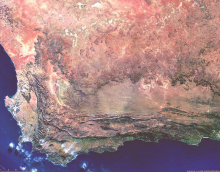
Articles

                                                                                                                                          Downloaded from https://academic.oup.com/bioscience/article-abstract/55/3/231/249703 by guest on 27 February 2020
                 Figure 1. Example of a bioclimatic model for Protea lacticolor, a species endemic to the Cape
                 Floristic Region (shown in photograph inset). Present range retained in a 2050 climate change
                 scenario is indicated in green. Present range lost in the 2050 scenario is in red, while new
                 range projected to become suitable in 2050 is indicated in blue. Note range loss in the low-
                 lands, range retention in the uplands, and limited opening of new range at higher elevations.
                 Photograph: Colin Paterson-Jones.

potential effects of climate change on efforts to conserve            detailed information on current distribution of the proteas
species in protected areas, answering questions such as whether       (Rebelo 2001). This information is used in bioclimatic mod-
climate change will increase or decrease the number of species        els to establish how climate influences the current distribu-
in protected areas, how these changes will unfold over time,          tion of proteas and to model possible future changes (box 2).
and what species and areas will be most affected. In this                The proteas studied are endemic to the Cape, another at-
article, we review the results of this modeling effort, with          tribute important for multispecies modeling. Bioclimatic
emphasis on similarities with and differences from findings           models perform reliably only when the climate and distrib-
from other regions, and on implications for protected areas           ution information on which they depend is available for the
and their ability to constrain species extinctions as climate         entirety of a species’ range, thus defining the complete “cli-
changes.                                                              mate envelope” that the species currently finds suitable (Pear-
                                                                      son and Dawson 2003). Using information from only a
The Cape as an example of multispecies modeling                       portion of a species’ range may cause a bioclimatic model to
The Cape studies are an example of bioclimatic (or “niche”)           ignore potentially broader tolerances represented by the
modeling, which has been conducted for many species in                species’ range outside of the study area. For this reason, mod-
several regions of the world (table 1). The Cape studies assess       eling should be restricted to species endemic to a study region,
the impact of climate change on more than 300 species in              or should cover the full geographic range of the species in
the protea family (Proteaceae; Midgley et al. 2003). The              question.
proteas—many of which are internationally important in                   The proteas are important conservation targets owing to
the floral trade because of their large, colorful flowers and their   their endemism and ecological significance. The family Pro-
attractive fruits and foliage—are excellent subjects for mod-         teaceae is one of the three floral elements that defines the fyn-
eling biotic responses to future climate shifts because they are      bos, a vegetation type so diverse that it makes the region
well studied and have life histories that make them directly sen-     surrounding the Cape of Good Hope the world’s smallest plant
sitive to climate change (Midgley et al. 2001). All successful        kingdom (Richardson et al. 2001). Proteas are the largest and
bioclimatic modeling efforts depend on information on the             showiest of the fynbos signature elements (Cowling 1992). The
current distribution of the species of interest. In the Cape, the     other defining fynbos elements are the ericas (Ericaceae),
Protea Atlas Project, an extensive cataloguing effort, provides       members of the heath family that have dwarf-shrub growth

232 BioScience • March 2005 / Vol. 55 No. 3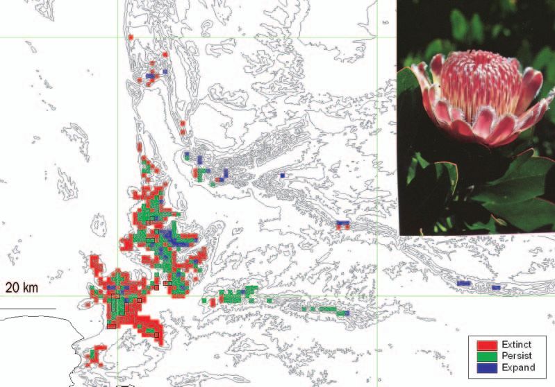
Articles

                                                    Box 1. Bioclimatic models:
                                             Climate change and species’ range shifts.

   Many assessments of the impact of climate change on biodiversity begin by creating bioclimatic models of a species’ present and pro-
   jected future range. Bioclimatic models establish a relationship between a species’ current distribution and climate. That relationship
   may then be extrapolated to simulated future climates, giving an estimate of the species’ possible future range. The simplest bioclimatic
   model creates a “climate envelope” for the species using the maximum and minimum values of various climate variables found within
   the species’ range (Box 1981); a popular variation of this type of model is BIOCLIM. A variety of techniques may be used to establish a
   relationship between a species’ distribution and environmental variables, including statistical approaches such as ordinary regression,
   generalized regression (e.g., generalized linear modeling, or GLM, and generalized additive modeling, or GAM), ordination (e.g., canon-

                                                                                                                                                    Downloaded from https://academic.oup.com/bioscience/article-abstract/55/3/231/249703 by guest on 27 February 2020
   ical correspondence analysis), and classification (e.g., classification and regression trees) as well as more complex techniques such as
   Bayesian frameworks, genetic algorithms, and artificial neural networks. For a detailed summary see Guisan and Zimmerman (2000).
   Bioclimatic models have limitations, but are useful for assessing vulnerability and spatial dynamics. Limitations include the assumptions
   that species’ ranges are in equilibrium with climate and that competition is a minor determinant of species’ ranges relative to climate
   (Pearson and Dawson 2003). Both of these assumptions are debatable, vary from species to species, and are difficult to test. Another
   limitation stems from modeling range instead of populations. A species’ range is comprised of a geographic extent (a polygon enclosing
   all occurrences, also known as extent of occurrence) and an area of occupancy—the habitats actually occupied within the geographic
   extent. Some bioclimatic models produce a probability surface of the species’ likelihood of occurrence. This probability is often convert-
   ed to a presence–absence surface by applying a cutoff value to yield a final product that is similar in appearance to a traditional range
   map (e.g., figure 1). At a coarse scale, the resultant map resembles the species’ extent of occurrence, as does a range map in a typical field
   guide. However, at a fine scale, the resulting map approximates the area of occupancy for the species (the habitats within the extent of
   occurrence that the species actually occupies). The Cape modeling was conducted using data at a resolution of 1 minute (approximately
   1.6 kilometers) by 1 minute, making it fine-scale relative to most bioclimatic modeling efforts but still coarse-scale relative to the area of
   occupancy of many plant species.

forms and small tubular or bell-shaped flowers, and the                      species responses (range expansion and contraction) in ar-
restios (Restionaceae), reed-like plants that resemble horse-                eas where the biome is projected to contract, as well as in ar-
tails. The fynbos has arisen in the mediterranean climate                    eas where the biome is projected to be retained (Midgley et
and rugged, mountainous terrain of the Cape, and some evi-                   al. 2002).
dence suggests that some groups have diversified and speci-                      Warming trends have already been observed in the Cape
ated widely in the geologically short period since the Miocene               region over the past 30 years by one of the authors (G. M.),
(Richardson et al. 2001). Most soils of the Cape are nutrient                working with Stephanie Wand. The Cape may therefore serve
poor, forcing adaptation and specialization in the plants that               in many ways as a harbinger of climate change effects else-
occur there, and the vegetation that has developed is prone                  where. The fate of the protected areas of the Cape offers
to fierce fires that recur at intervals of 10 to 30 years (Cowl-             lessons that can inform conservation efforts throughout the
ing 1992). Strong winds whip the Cape region, creating                       world.
unique conditions for fire and plant dispersal, factors that are
central to the diversity of the region (Simmons and Cowling                  Extinction risk and multispecies modeling
1996).                                                                       Extinction risk for the proteas of the Cape due to climate
   Species are the unit of study in the Cape protea modeling                 change alone has been estimated at 21% to 40%, using
because abundant evidence from the past indicates that                       midrange scenarios of greenhouse gas emissions (Thomas et
species respond individually to change in climate, rather                    al. 2004). The species–area relationship calculations on which
than as coherent communities. No-analog communities—as-                      these estimates are based remain the subject of debate (box
sociations of prehistoric
plants or animals that are          Table 1. Multispecies (n ≥ 50) bioclimatic modeling efforts.
unlike any that currently           Region              Taxa                         Number of species         Reference
exist—are a common feature          Europe              Plants                              192                Bakkenes et al. 2002
of the paleoecological record.      Europe              Plants                            1200                 Araujo et al. 2004
Modeling of the Cape has            Europe              Birds                               306                Huntley et al. 2004
                                    Britain and Ireland Plants                               54                Berry et al. 2002
been conducted at the com-          South Africa        Vertebrates, insects                 50                Erasmus et al. 2002
munity (biome) level, and           South Africa        Plants (Proteaceae)                 330                Midgley et al. 2003
this modeling shows a south-        Mexico              Birds, butterflies                1870                 Peterson et al. 2002
                                    Brazil              Trees                               163                Ferreira de Siqueira et al. 2003
ward collapse of the fynbos         Amazonia            Trees                                69                Miles et al. 2004
biome that contains the pro-        Australia           Vertebrates, insects                 65                Williams et al. 2003
teas. But species-level mod-        Canada              Butterflies                         111                Peterson et al. 2004
                                    United States       Trees                                80                Iverson and Prasad 1998
eling shows a variety of

                                                                                                  March 2005 / Vol. 55 No. 3 • BioScience 233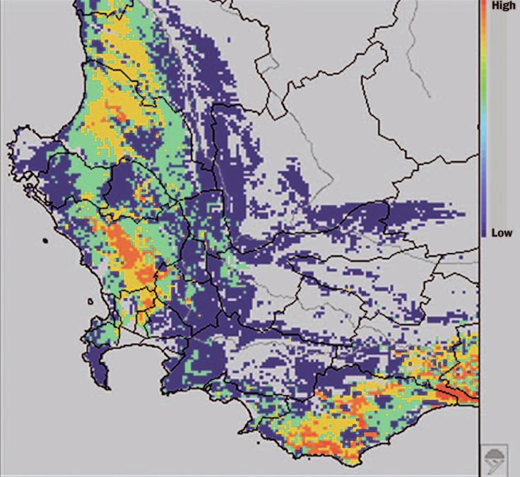
Articles
Downloaded from https://academic.oup.com/bioscience/article-abstract/55/3/231/249703 by guest on 27 February 2020
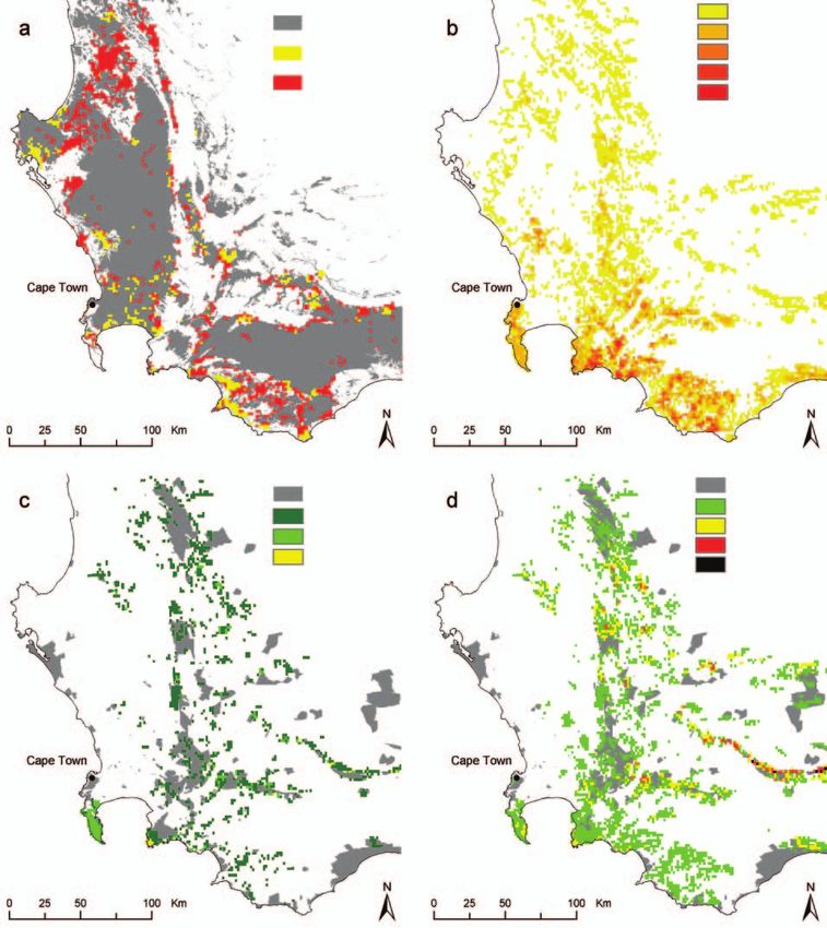
Figure 2. Satellite image of the Cape region. The outlined box indicates the approximate
location of figure 1. Note extensive north–south and east–west trending mountains of
the Cape fold belt. Source: Image courtesy of MODIS Rapid Response Project at
NASA/GSFC.
3; Harte et al. 2004, Thuiller et al. 2004). It has been suggested mate change. Over the coming decades, human land trans-
that extinction risk due to climate change might be better es- formation and fragmentation is likely to destroy most un-
timated by counting the number of species whose climatic protected natural habitats (figure 3a), while climate change
niche falls below a critical minimum size (Buckley and Rough- will accelerate, rendering many currently climatically suitable
garden 2004). In the real world, climate change will act in syn- areas unsuitable for particular species even within protected
ergy with other pressures, and most important will be the areas (figure 3d). The net remaining populations will be pri-
interaction of habitat loss with climate change. marily those that are protected from habitat loss in parks, re-
Extinction risk due to habitat loss is already high in the serves, and other conservation areas (conservancies on private
Cape, as evidenced by the number of threatened (Red List; lands are of growing importance in the Cape) and that can
IUCN 2001) protea species per unit area (figure 3b). At pres- withstand the loss of climatically suitable space within those
ent, more than 30% of the region has already been heavily refuges. Adopting the premise that extinction risk will be de-
transformed by agriculture, urbanization, and dense stands termined for individual species by the intersection of protected
of invasive alien plants, and much of the remainder has alien areas and climatically suitable space, we use the results of the
species present in low densities (figure 3a). Thirty percent of protea modeling to explore the complex conservation con-
the remaining natural habitat is threatened by future ex- sequences of climate change and land-use change for the
treme transformation (Rouget et al. 2003a). Some lowland proteas and protected areas in the Cape.
habitats have lost more than 80% of their original extent al-
ready and have less than 5% of their remaining extent pro- Protected areas and climate change
tected. Unsurprisingly, many proteas have disappeared from Bioclimatic models can be used to calculate the effect of cli-
heavily transformed areas, and for many species, conservation mate change on species representation in protected areas.
areas harbor their last remaining populations. Overall, some Current and future modeled ranges may be used to calculate
20% of the region is protected in some form of conservation the area of a species’ range under protection at a given time,
area, but only half of this is in reserves with a high degree of although it is important to keep in mind that a species’ mod-
protection (Rouget et al. 2003b). eled potential range may not precisely match its actual range
Conservation of the proteas will ultimately depend on (Pearson and Dawson 2003). As the climate changes, the
protected areas to maintain critical minimum population amount of range under protection will change, depending on
sizes of species against the incursions of habitat loss and cli- the changes in the species’ range relative to the geographic
234 BioScience • March 2005 / Vol. 55 No. 3Articles
01–5 Red List spp.
Transformed 2000
06–10
Transformed 2020 11–15
(best-case scenario)
18–20
Transformed 2020
(worst-case scenario) 21–26
Downloaded from https://academic.oup.com/bioscience/article-abstract/55/3/231/249703 by guest on 27 February 2020
Protected areas
Protected areas
+1–2 Red List spp.
+1 Red List spp.
+3–4
+2
+5–6
+3
+7–8
Figure 3. (a) Extent of habitat transformation in the southwestern Cape Floristic Region in 2000 and additional pro-
jected habitat transformation by 2020, assuming a low transformation rate (best-case scenario) and a high transfor-
mation rate (worst-case scenario) (Bomhard et al. 2005). (b) Number of species on the IUCN Red List (IUCN 2001) per
1-minute grid cell (2.9 km2) for 227 protea taxa endemic to the Cape Floristic Region. (c) Protected areas and increase
in the number of Red List proteas per grid cell, based on a Red List assessment (IUCN 2001) that incorporates projected
worst-case land-use change by 2020. (d) Protected areas and increase in the number of Red List proteas per grid cell,
based on a 2020 Red List assessment that incorporates both land-use and climate change.
location of protected areas. Projecting the change in climate resultant impacts on climate projected by general circulation
carries considerable uncertainty. Future emissions of green- models (GCMs) vary considerably (IPCC 2001). These un-
house gases into the atmosphere can only be estimated certainties are critical to the global policy debate on con-
(through emissions scenarios; IPCC 1996, 2001), and the straining climate change, but multiple emissions scenarios and
March 2005 / Vol. 55 No. 3 • BioScience 235Articles
mechanism (wind, rodent, or ant dispersal) and estimated the
Box 2. The Cape protea models. likely maximum dispersal distance in 10-year time steps over
50 years. Most bioclimatic modeling studies use dual
assumptions of “no dispersal” or “universal dispersal” (e.g.,
The models of protea range shifts conducted for the Cape
Peterson et al. 2002). Contiguous dispersal (dispersal into ad-
are among the most detailed ever undertaken. Three key
ingredients are required for such models: (1) species distri- jacent cells) is sometimes used (e.g., Peterson 2003), but it has
bution data, (2) fine-scaled present and future climate data, limitations of its own, namely that it is arbitrarily linked to
and (3) data on other environmental variables (e.g., soil time step and spatial scale of modeling. The no-dispersal
data) (Hannah et al. 2002b). and maximum-dispersal assumptions used for the Cape pro-
tea modeling are a compromise that discounts the importance
Species distribution data for the proteas came from the
Downloaded from https://academic.oup.com/bioscience/article-abstract/55/3/231/249703 by guest on 27 February 2020
of unlikely long-distance dispersal events, the role of which
Protea Atlas Project (Rebelo 2001). The data from this pro-
ject make it possible to model future range shifts of the pro- remains controversial (Clark et al. 2003). The maximum-
teas. The Protea Atlas Project provides records of species’ dispersal assumption is different from universal dispersal, in
presence and absence over large areas of the Cape. These that it limts dispersal to range that is climatically suitable
records can be used to train a statistical model to predict and within a maximum distance based on whether the species
the distribution of a species on the basis of key climate and is dispersed by wind, ants, or rodents in each of five decadal
soil variables. Once the variables most strongly influencing time steps. The no-dispersal assumption is simply the over-
present distribution are determined, it is possible to assess lap of the future range with the present range, which is crit-
how a species’ range might shift under future climate ical for protected areas and conservation because it
change. corresponds to the areas in which climate is projected to re-
The South African national study on climate change pro- main suitable for a species.
vided fine-scale present and future climate data based on The Cape protea models suggest that, if the current
projections from a global climate model (general circula- protected-area network does not change before 2050, the
tion model, or GCM) (Midgley et al. 2002). The future cli- number of species represented in the protected areas of
mate variables were derived from coarse-scale projections the region in the future depends strongly on dispersal
of the GCM known as HadCM2 (Hadley Centre coupled assumption (table 2). In the Cape, the number of protea
model version 2), which were converted to 1-minute resolu-
species in protected areas declines by 15% assuming no dis-
tion using a statistical downscaling technique (Midgley et
persal, and by 8% assuming maximum dispersal. In the only
al. 2002). Information on other environmental variables,
such as soils, elevation, land-cover classes, and protected comparable study of large numbers of species, Araujo and col-
areas, from a GIS (geographic information system) database leagues (2004) found that 6% to 10% of European plant
completed the information used in the Cape studies. species would be lost from reserves as a result of climate
changes projected for 2050 (the lower estimate associated
Several categories of bioclimatic models exist for projecting
with a universal-dispersal scenario).
changes in a species’ range as climate shifts (box 1). The
These findings are significant for two reasons. First, the
Cape protea models were constructed using generalized
additive modeling (GAM). GAM creates a statistical rela- number of protected species declines in the Cape even under
tionship between present range and present climate, then the maximum-dispersal scenario. Climate change will certainly
extrapolates future range on the basis of changes in climate rearrange species relative to protected areas, but it is not a
variables projected by the GCM (figure 1). This process was foregone conclusion that this rearrangement will decrease
followed for over 300 species of protea, producing a fine- the number of protected species. Some species will have
scale, multispecies look at possible changes in biodiversity future potential range within protected areas in which they
due to climate changes expected by 2050 (Midgley et al. do not currently occur. Others may exchange protected area
2002). in one part of their present range for protected area in a dif-
ferent reserve in their potential future range. In theory, the net
GCMs can greatly complicate general understanding of un- effect of these changes could be neutral, or could even result
derlying patterns of climate-change impacts on species and in expanding representation of species in protected areas.
protected areas. Here we treat species and protected areas first, Whether the potential future range could ever be occupied
using a single emissions scenario and the GCM from the when species have to cross future heavily transformed and
Cape assessment (HadCM2, or Hadley Centre coupled model fragmented landscapes would then be debatable. But the
version 2) for simplicity, and then return to the issues of pol- Cape results show that even before species get to the challenge
icy and uncertainty. of crossing hostile intervening landscapes, the number of
A species’ range may shrink in response to climate change species in protected areas is reduced by climate change. The
in an area where it is currently protected, but it may also ex- results of Araujo and colleagues (2004) for Europe support
pand in areas where it is not currently protected. Whether or this interpretation.
not a species has the dispersal capacity to reach newly suit- The decline in the number of protected species is due to an
able range has a major impact on the size of future range, so overall strong decline in species range size with climate
we divided the proteas on the basis of primary dispersal change. Part of this decline results from the dispersal constraint
236 BioScience • March 2005 / Vol. 55 No. 3Articles
Table 2. Numbers of endemic protea species represented in protected areas of the Cape Floristic
Region in 2000 and 2050 (projected).
Number of species (percent decline since 2000)
Year (threshold) No-dispersal assumption Maximum-dispersal assumption
2000 (presence only) 327 (0) –
2050 (presence only) 277 (15.3) 301 (8.0)
2050 (100-km2 minimum threshold) 202 (38.2) 243 (25.7)
Note: The number of species whose modeled ranges intersect protected areas in at least one grid cell (presence only)
or at a minimum threshold of area (100 km2) are given relative to two dispersal assumptions about species’ ability to
Downloaded from https://academic.oup.com/bioscience/article-abstract/55/3/231/249703 by guest on 27 February 2020
occupy newly climatically suitable areas.
placed on potential future range, but the pattern of overall de- present, while a few have much greater ranges protected.
cline exists even when this constraint is removed (Midgley et This is another important lesson from the Cape studies:
al. 2003). This effect has been demonstrated in multiple re- most species are projected to become rarer, while a few will
gions of the world, and the Cape is a good illustration of this prosper and become more widespread. This phenomenon has
pattern (Thomas et al. 2004). Similar findings have been re- been noted in several other multispecies modeling efforts,
ported for other regions and species of South Africa (Eras- including regions as diverse as Mexico (Peterson et al. 2002)
mus et al. 2002); Queensland, Australia (Williams et al. 2003); and Britain and Ireland (Berry et al. 2002). The loss of species
and Brazil (Ferreira de Siqueira and Peterson 2003). A represented in protected areas by 2050 is modest, but is
major reason for this decline is that in warming climates, underlain by a deeper erosion of protected range that will turn
species move upslope into smaller and smaller areas as moun- into an explosion of unprotected species as climate change
tain peaks taper at higher elevations. The present global continues beyond 2050.
climate is at a warm interglacial level, one of the warmest Loss of protected range may be compared with overall
in the past 2 million years, and future warming will push loss of species’ ranges, to see whether protected areas are far-
species further upslope as climate becomes the warmest in ing better or worse than the overall landscape. In compari-
40 million years or more (Overpeck et al. 2003). This son with overall range losses, the protected-range losses are
effect may be particularly strong in the Cape, since there is less (36% to 72% compared with 57% to 86%) for the pro-
no poleward continental landmass in which latitudinal teas. This is the result of the predominance of mountainous
range adjustments might take place. protected areas. Species are moving upslope with warming,
The decline in number of protected species masks an even and most protected areas are in the mountains. Therefore, the
deeper erosion of protected-area effectiveness. Among those upslope portion of a species’ range loses less area to climate
species that are represented in protected areas, the increased change and is more protected, resulting in less loss in the
vulnerability to extinction due to reduced range size that ac- protected parts of the range. This lesson from the Cape is not
companies climate change may be examined by looking at the universally applicable but is universally relevant: regions that
area of species’ ranges protected at present and in the future have predominantly lowland reserves will see dispropor-
(table 3). Mean protected range of protea species declines by tionately larger losses of protected range, while regions with
36% to 60% under the future climate scenario. Declines in me- abundant upland reserves, like the Cape, will see lesser losses
dian protected range are markedly larger (39% to 72%), par- of protected range.
ticularly under the no-dispersal scenario. The differences
between median and mean values in the present indicate How much is enough?
that protection is currently skewed toward species with small Protected areas are a mainstay of conservation, and their
ranges. This bias in the distribution of protected range be- utility relies on the assumption that extinction debt due
comes even more pronounced in the future. In the 2050 sce- either to habitat loss or to climate change can be forestalled
nario, many species have smaller protected ranges than at within relatively small areas of the landscape if those areas are
Table 3. Mean and median size of protected range of protea species modeled, with mean and median
total modeled range size for comparison.
Range size (km2) in protected areas Total range size (km2)
(percent decline since 2000) (percent decline since 2000)
Year (threshold) Mean Median Mean Median
2000 (present range) 358 (0) 206 (0) 1948 (0) 1454 (0)
2050 (no dispersal; overlap of 144 (59.8) 58 (71.8) 495 (74.6) 211 (85.5)
present and future range)
2050 (maximum dispersal) 228 (36.3) 126 (38.8) 845 (56.6) 362 (75.1)
March 2005 / Vol. 55 No. 3 • BioScience 237Articles
age to biodiversity conservation may be the more realistic. Sig-
Box 3. Species–area relationships
nificantly larger investments in protected areas and their
and climate change.
management may be required to avoid extinctions due to cli-
mate change.
The species–area relationship (SAR) is an empirical rela-
But how much more is enough? Arriving at an answer to
tionship between the number of species and the land area
of a continent or island. The larger the area, the more this question for the future is difficult, because there is no
species, as one might expect; in many settings, this relation- agreed-upon standard for the present. Where population
ship is approximately linear when both scales (area and viability analyses have been conducted (e.g., for threatened
number of species) are log transformed. A variant of the species), a good approximation of the amount of habitat
SAR is the endemics–area relationship (EAR), which (range) required for a species’ conservation may be avail-
Downloaded from https://academic.oup.com/bioscience/article-abstract/55/3/231/249703 by guest on 27 February 2020
describes the relationship between land area and the num- able. For the vast majority of species, however, these data do
ber of species endemic to a region (Kinzig and Harte 2000). not exist (Noss 1996). Simple presence is an inappropriate met-
In both SAR and EAR, the slope of the log-transformed ric, as a single occurrence is unlikely to support a viable pop-
line, or z value, is the critical determinant of how species ulation for most species. A blanket percentage of range is
accumulate as area is added.
unlikely to be appropriate, as different species have different
Thomas and colleagues (2004) used SAR in a novel way to range requirements. The current degree of protection (for
estimate extinction risk from climate change. These authors species that are represented in the protected-area system)
theorized that because species accumulate as one moves to is one possible but largely arbitrary benchmark—most
larger and larger island or continental areas, the converse current protected-area networks have not been systematically
must also be true—species must be lost as their climatically designed, so some species are vastly overrepresented while
suitable space becomes progressively smaller. A similar
others are vastly underrepresented.
assumption had been used to estimate the number of
Protecting all the remaining range of species below a min-
extinctions that would eventually occur as the result of
habitat loss (Brooks et al. 1999). imum rarity threshold has been suggested as a goal (Noss
1996). For assessing critically endangered species, the IUCN
The SAR approach to estimating extinction risk from cli- (the World Conservation Union) has set a threshold for rar-
mate change has attracted criticism. Unlike other researchers ity at 100 km2 extent of occurrence (IUCN 2001). This 100-
who used SAR to estimate species losses due to habitat loss,
km2 minimum threshold is used in table 2 to illustrate the
Thomas and colleagues (2004) calculated range loss for
difference between using a target threshold and using simple
each species individually, then used several alternative
methods to estimate aggregated extinction risk. Some presence (at the scale of the study) as a criterion for protec-
authors have argued that the aggregation methods used by tion. Until conservationists can answer the question “How
Thomas and colleagues were not correct, while others have much is enough?” in the present, it will be impossible to gen-
argued that combining individual range changes is not a erate more precise estimates of protected-area requirements
valid use of SAR at all (Buckley and Roughgarden 2004). to compensate for climate change.
Thomas and colleagues addressed only endemic species, so
that they could be sure their bioclimatic models were able Which species and when?
to address all of a species’ range, and it has been pointed In the Cape models, lowland species and species with small
out that EAR might have been more appropriate to apply ranges lose protection first. This pattern follows the trend for
than SAR in this case.
small-range and lowland species to lose the most range, re-
gardless of whether the range is in protected areas or outside.
properly protected and managed. How much area is enough The present range sizes of species that are lost from the pro-
remains a largely unanswered question in conservation, how- tected areas are much smaller than those of the species that
ever. Biologically meaningful targets at the regional and na- are retained. Protea species projected to lose all protected
tional levels have been elusive, while data deficiencies limit the range have a mean range size of 2290 km2, compared with the
ability to estimate the area needs of individual species (Soulé mean range size of 5590 km2 for all species. This is consistent
and Sanjayan 1998). with the theory suggesting that species with smaller ranges will
The extent of protection required matters greatly in terms have a smaller envelope of environmental variables within that
of how many species are lost from protected areas as a result range, and hence greater sensitivity to climate change (Hughes
of climate change. In the Cape, if a single small area (under 1996, Pimm 2001).
3 square kilometers [km2] at the resolution of this study) is Lowland species are also disproportionately affected. Fig-
sufficient for species persistence, then only 8% to 15% of ure 4 shows the species richness of species that lose all pro-
proteas are projected to be lost from protected areas (de- tection. Lowland species dominate, while only a few montane
pending on the dispersal assumption), whereas 26% to 38% species lose all protection; large parts of the Cape fold moun-
of species are projected to be lost if species persistence requires tains are outlined in cool, low-richness blue. This follows
a substantially greater area (table 2). Since most species require the general pattern for proteas in the Cape, in which most low-
substantial area to maintain a viable population and resist land species rapidly lose range—possibly because the Cape’s
chance extinctions, the higher estimates of the possible dam- situation at the southern tip of the African continent makes
238 BioScience • March 2005 / Vol. 55 No. 3Articles
Downloaded from https://academic.oup.com/bioscience/article-abstract/55/3/231/249703 by guest on 27 February 2020
Figure 4. Richness of species that lose all protected range in the southwestern Cape
Floristic Region. Warmer colors indicate higher numbers of species. Worldmap software
and map courtesy of Paul Williams.
latitudinal adjustments poleward largely impossible. Other The timing of species loss under different dispersal
studies in regions where latitudinal adjustments are possible assumptions in the Cape is illustrated in figure 5. No-dispersal
have noted losses in lowland species range ranging from protected range (future protected range that overlaps with
moderate (Peterson et al. 2002) to pronounced. current protected range) is lost first and continues to de-
This “lowland loss” effect is in apparent conflict with other cline, while the loss of protected range under the maximum-
estimates that most extinctions due to climate change will oc- dispersal assumption starts more slowly and levels off with
cur in mountains, as species moving upslope find less and less time. This is because species’ ranges move into the Cape fold
habitat, and eventually have nowhere to go. In fact, both per- mountains and then track the changing climate by moving
spectives may be correct. Required migration distances for to other parts of the mountain chain. Future new range
range shifts due to climate change are shorter in uplands, opens up in montane reserves, causing the protected-range
loss to decrease if species are assumed to be able to realize their
where steep climatic gradients prevail, than in lowlands,
maximum dispersal potential. Protected range under the no-
which have a more uniform climate. Although lowland species
dispersal assumption, on the other hand, exhibits continuous
therefore suffer a larger absolute range loss, they usually ex-
decline, as overlap between present and future range pro-
hibit a lower extinction risk, because many of them tend to gressively erodes. Although the absolute level and rate of cli-
be widespread (Dynesius and Jansson 2000). Many upland mate change are likely to be different from those shown in this
species, in contrast, have relatively small range sizes, so that graph because of uncertainties in climate models and emis-
a major proportional range loss leaves them with little absolute sions scenarios, this relative pattern is likely to be robust in
range and a higher extinction risk. Effects in both lowlands the Cape under all model and scenario combinations, because
and uplands will depend strongly on patterns of land use (Pe- of the extensive and well-protected mountains of the region.
terson 2003). Even widespread lowland species with good dis- The distinctive L shape of the Cape mountains, extending both
persal ability may face extinction if extensive transformed and north–south and east–west (figure 2), provides expanding
fragmented landscapes (figure 3a) lie between their present areas of refuge to the east as species ranges move south,
and future ranges. which is unusual. In most montane settings, steady loss of
March 2005 / Vol. 55 No. 3 • BioScience 239Articles
lands that could be considered as candidates for protection.
In addition to the species that have no overlap range protected,
a further 12 species have less than 1000 hectares (ha) of over-
lap range in protected areas, but substantial (more than 1000
ha) of overlap range outside of protected areas in untrans-
formed areas suitable for conservation.
Number of species
For species unrepresented in the current protected-area net-
work, protecting their overlap range offers a double oppor-
tunity. The representation of their 2050 overlap range can be
improved, and at the same time their present range can be rep-
Downloaded from https://academic.oup.com/bioscience/article-abstract/55/3/231/249703 by guest on 27 February 2020
resented in protected areas for the first time. In the case of the
Cape proteas, however, this promise goes unfulfilled. All of the
protea species unrepresented in the current protected areas
of the Cape have very small present ranges. Like other small-
range species, their ranges quickly disappear as the climate
changes, and they are projected to have no range at all in 2050.
Thus, portions of their present range may be captured in
protected areas, but their future modeled ranges appear to pre-
2000 sent no opportunity for overlap conservation.
Year In sum, a significant but limited proportion of the proteas
that have no overlap range in the current protected-area net-
Figure 5. Number of protea species protected through work might be saved through new protected areas. Other
time according to a model of the Cape Floristic Region, measures will be necessary to ensure the conservation of the
showing number of species with 100 square kilometers remaining species. As climate change progresses, the number
(km2) of protected total range (diamonds) and with 100 of species requiring extraordinary measures will increase.
km2 of overlap between protected present and future
range (i.e., no-dispersal assumption; squares). Conservation implications
In regions such as the Cape, not only the climate will change;
range over time (due to decreasing area at higher elevations) human population and the resulting pressures on ecosystems
even with maximum dispersal, such as that observed by will continue to evolve, often in ways unfavorable to bio-
Williams and colleagues (2003) in upper montane species of diversity. The synergies between these multiple changes will
Queensland, Australia, is probably the norm. In nonmontane ultimately have major implications for conservation. For ex-
regions, loss of range under all dispersal assumptions may be ample, agriculture in the Cape may move upslope to retreat
rapid, as discussed above. from the warming and drying lowlands and to retain optimal
These patterns of vulnerability and timing are consistent environmental conditions for crops (e.g., optimal tempera-
with upslope and poleward movements expected with warm- ture for vineyards or cold duration for orchard fruits), in
ing. In the Cape, warming dominates the modeled biotic re- the process destroying natural habitats in areas that today are
sponses to future climate change, as it does in many other of little agricultural value. In addition, climate change and
systems that have been modeled. In other regions, precipita- growth-stimulating effects of rising carbon dioxide (CO2) may
tion may be more important. For example, precipitation accelerate the spread of invasive alien plants, which already
changes and interruption of moisture recycling have been im- outcompete slow-growing and CO2-nonresponsive indigenous
plicated in the modeled retreat of Amazonian forests under fynbos plants in many areas of the Cape, with serious impli-
future climate change (Betts et al. 1997, Miles et al. 2004). cations for water resources and fire regimes. Much of the
protected range in the maximum-dispersal scenarios dis-
Can more protected areas compensate? cussed above could never be occupied because of present in-
Species whose future range has no overlap with their present compatible land uses, and land use will continue to change,
range may have trouble tracking climate change, even when often in response to changing climate.
their future range is projected to be substantial. Overlap More than twice as many additional proteas may be threat-
between present and future range is therefore an important ened if land use and climate change are considered together,
attribute to represent in protected areas. This overlap range compared with estimates considering changes in land use
is equivalent to the range under the no-dispersal assumption. alone. Presently, 126 of the proteas modeled are classified as
In the Cape, a few species that are projected to lose all threatened (critically endangered, endangered, or vulnerable)
protected overlap range by 2050 have untransformed but according to Red List criteria (IUCN 2001). If only
unprotected overlap range that could be protected to fill the future land-use change as predicted for 2020 is considered,
gap. Of the 62 proteas that have no protected overlap range 4 to 13 additional species would be classified as threatened,
in 2050, 20 have overlap range outside of protected areas on compared with an additional 30 to 37 species if land use and
240 BioScience • March 2005 / Vol. 55 No. 3Articles
climate change are considered together (no-dispersal as- conservation tools such as the IUCN Red Lists of threatened
sumption) (Bomhard et al. 2005). The spatial distribution of species, the consideration of future threats to biodiversity may
these species is remarkable (figure 3). Compared with a Red not be adequate at present, given the challenge ahead.
List assessment that does not look into the future, the num- Ultimately, improved conservation responses must be ac-
ber of Red List proteas could rise by up to three species per companied by global policies to halt climate change. The
1-minute grid cell because of future land use change alone (fig- Kyoto Protocol is now in force, a tremendous step in collab-
ure 3c). The number of Red List proteas could, however, rise oration and collective international action, but a small step
by up to eight species per 1-minute grid cell, if climate- in substantive reduction of greenhouse gas emissions. The
change effects as predicted for 2020 are added to the land-use challenge ahead is staggering—halting climate change, the crit-
change effects on species’ ranges (figure 3d), with consider- ical goal for biodiversity, requires stabilizing atmospheric
Downloaded from https://academic.oup.com/bioscience/article-abstract/55/3/231/249703 by guest on 27 February 2020
able changes occurring within and outside protected areas. The greenhouse gas concentrations. A stable level of greenhouse
good news is that the predominance of mountainous pro- gases in the atmosphere implies zero net emissions, which
tected areas seems already to provide critical refuge for some would require the total transformation of the global energy
upland species affected by future climate change. However, supply system to renewable sources. Accomplishing this in the
for many lowland species, and for upland species outside space of several decades without huge environmental costs is
current protected areas, there is no such good news. a gargantuan task (Lackner 2003). Biologists need to be in-
Why does this matter? Conservation planning for additional formed and engaged in the global debate about climate
reserve site selection, for example, is heavily based on avail- change, or these changes may overwhlem hard-won and still
able information on the distribution of threatened species and incomplete gains in habitat protection. The ultimate solutions
ecosystems. Knowledge of future changes in the distribution are not immediately apparent, but this is not a reason to
of threatened species can certainly help to identify those avoid action, but rather an imperative to engage now and help
areas that hold the maximum potential for biodiversity con- formulate solutions that work for society and biodiversity.
servation in the face of future threats. Furthermore, knowl- Biologists, particularly those in the United States, have a
edge of where, when, and how future threats may affect stake in advocating this course.
species can help to identify the most appropriate conserva- Climate change is a dangerous and uncertain game for bio-
tion measures for each species. Species most affected by diversity. We know that the present ranges and the present de-
climate change are likely to require additional measures (e.g., gree of protection of many species will rapidly erode as a result
facilitated range shifts) compared with those most affected by of climate change. The degree to which these losses can be
land-use change, which can be saved through protection of compensated for by occupation of newly suitable range is
their remaining natural habitat. Improved conservation highly uncertain. Some refinements to protected-area net-
strategies can compensate for some of the future changes, but works can clearly reduce the damage that might be expected
clearly even the most forward-looking of these strategies will by mid-century. Past that, uncertainty rises, but considerable
break down in the face of unlimited change. negative consequences for biodiversity loom. The only sure
For species without overlap range, one possible conserva- way of improving the odds is to limit climate change itself—
tion strategy is the creation of corridors that will allow species a huge task with huge benefits for biodiversity and, ulti-
to track climate changes (Hannah et al. 2002a). Another is mately, for all of us.
moderate to intensive management to maintain populations
and facilitate range shifts through translocation. Either strat- Acknowledgments
egy will require major new resources. Corridors carry un- The authors gratefully acknowledge Tony Rebelo and the
certainty, as it is unknown whether all species will be able to Protea Atlas Project for providing the data that made these
migrate fast enough to track climate change of the magnitude analyses possible, and Paul Williams for providing the
projected for the coming century. However, it is possible to Worldmap conservation planning software and visualiza-
identify “chains” or “tracks” of suitable habitat for species tions. A View from the Alps (MIT Press, 1998) inspired our
migration using bioclimatic models. Areas in which these title.
tracks overlap for many species could be protected as corri-
dors for multispecies migration (Williams et al. 2003). The References cited
alternative—intensive management—may be incompatible Araujo MB, Cabeza M, Thuiller W, Hannah L, Williams PH. 2004. Would
with the conservation of natural processes in many areas, but climate change drive species out of reserves? An assessment of existing
reserve-selection methods. Global Change Biology 10: 1618–1626.
it could have a higher likelihood of successful conservation Bakkenes M, Alkemade JR, Ihle F, Leemans R, Latour JB. 2002. Assessing the
of species. effects of forecasted climate change on the diversity and distribution of
European higher plants for 2050. Global Change Biology 8: 390–407.
Regional change and global policy Berry PM, Dawson TP, Harrison PA, Pearson RG. 2002. Modelling poten-
For biodiversity conservation, it is time to take these future tial impacts of climate change on the bioclimatic envelope of species in
Britain and Ireland. Global Ecology and Biogeography 11: 453–462.
changes into account when developing climate change– Betts RA, Cox PM, Lee SE, Woodward FI. 1997. Contrasting physiological
integrated conservation strategies (“adaptation” measures in and structural vegetation feedbacks in climate change simulations.
IPCC parlance) (Hannah et al. 2002a, 2002b). In widely used Nature 387: 796–799.
March 2005 / Vol. 55 No. 3 • BioScience 241Articles
Bomhard B, Richardson DM, Donaldson JS, Hughes GO, Midgley GF, Midgley GF, Hannah L, Millar D, Thuiller W, Booth A. 2003. Developing
Raimondo DC, Rebelo AG, Rouget M, Thuiller W. 2005. Potential regional and species-level assessments of climatic change impacts on bio-
impacts of future land use and climate change on the Red List status of diversity in the Cape Floristic Region. Biological Conservation 112:
the Proteaceae in the Cape Floristic Region, South Africa. Global Change 87–97.
Biology. Forthcoming. Miles L, Grainger A, Phillips O. 2004. The impact of global climate
Box EO. 1981. Macroclimate and Plant Forms: An Introduction to Predic- change on tropical forest diversity in Amazonia. Global Ecology and
tive Modelling in Phytogeography. The Hague: Junk. Biogeography 13: 553–565.
Brooks TM, Pimm SL, Oyugi JO. 1999. Time lag between deforestation and Noss RF. 1996. Protected areas: How much is enough? Pages 91–120 in
bird extinction in tropical forest fragments. Conservation Biology 13: Wright RG, ed. National Parks and Protected Areas. Cambridge (MA):
1140–1150. Blackwell.
Buckley LB, Roughgarden J. 2004. Biodiversity conservation: Effects of Overpeck J, Whitlock C, Huntley B. 2003. Terrestrial biosphere dynamics in
changes in climate and land use. Nature 430 (6995). (1 February 2005; the climate system: Past and future. Pages 81–109 in Alverson KD,
Downloaded from https://academic.oup.com/bioscience/article-abstract/55/3/231/249703 by guest on 27 February 2020
www.nature.com/cgi-taf/DynaPage.taf?file=/nature/journal/v430/ Bradley RS, Pederson TF, eds. Paleoclimate, Global Change, and the
n6995/full/nature02719_fs.html)
Future. Berlin: Springer-Verlag.
Clark JS, Lewis JS, McLachlan JS, Lambers JH. 2003. Estimating population
Parmesan C, Yohe G. 2003. A globally coherent fingerprint of climate change
spread: What can we forecast and how well? Ecology 84: 1979–1988.
impacts across natural systems. Nature 421: 37–42.
Cowling RM. 1992. The Ecology of Fynbos: Nutrients, Fire and Diversity. Cape
Pearson RG, Dawson TP. 2003. Prediciting the impacts of climate change on
Town (South Africa): Oxford University Press.
the distribution of species: Are bioclimate envelope models useful?
Dynesius M, Jansson R. 2000. Evolutionary consequences of changes in
Global Ecology and Biogeography 12: 361–371.
species’ geographical distributions driven by Milankovitch climate
oscillations. Proceedings of the National Academy of Sciences 97: Peters RL, Darling JD. 1985. The greenhouse effect and nature reserves.
9115–9120. BioScience. 35: 707–717.
Erasmus BFN, Van Jaarsveld AS, Chown SL, Kshatriya M, Wessels KJ. 2002. Peterson AT. 2003. Projected climate change effects on Rocky Mountain
Vulnerability of South African animal taxa to climate change. Global and Great Plains birds: Generalities of biodiversity consequences. Global
Change Biology 8: 679–693. Change Biology 9: 647–655.
Ferreira de Siqueira M, Peterson AT. 2003. Global climate change consequences Peterson AT, Ortega-Huerta MA, Bartley J, Sanchez-Cordero V, Soberon J,
for Cerrado tree species. Biota Neotropica 3: 1–14. Buddemeier RH, Stockwell DR. 2002. Future projections for Mexican
Guisan A, Zimmermann NE. 2000. Predictive habitat distribution models in faunas under global climate change scenarios. Nature 416: 626–629.
ecology. Ecological Modelling 135: 147–186. Peterson AT, Martinez-Meyer E, Conzalez-Salazar C, Hall PW. 2004.
Hannah L, Midgley GF, Lovejoy TE, Bond WJ, Bush M, Lovett JC, Scott D, Modeled climate change effects on distributions of Canadian butterfly
Woodward FI. 2002a. Conservation of biodiversity in a changing species. Canadian Journal of Zoology 851–858.
climate. Conservation Biology 16: 264–268. Pimm SL. 2001. Entreprenurial insects. Nature 411: 531–532.
Hannah L, Midgley GF, Millar D. 2002b. Climate change–integrated Rebelo AG. 2001. Proteas: A Field Guide to the Proteas of Southern Africa.
conservation strategies. Global Ecology and Biogeography 11: 485–495. Cape Town (South Africa): Fernwood Press.
Harte J, Ostling A, Green JL, Kinzig A. 2004. Biodiversity conservation: Cli- Richardson JE, Weitz FM, Fay MF, Cronk QCB, Linder HP, Reeves G, Chase
mate change and extinction risk. Nature 430 (6995). (1 February 2005; MW. 2001. Rapid and recent origin of species richness in the Cape Flora
www.nature.com/cgi-taf/DynaPage.taf?file=/nature/journal/v430/ of South Africa. Nature 412: 181–183.
n6995/full/nature02718_r.html&filetype=&dynoptions=) Root TL, Schneider SH. 1995. Ecology and climate: Research strategies and
Hughes L, Cawsey EM, Westoby M. 1996. Climate range sizes of Eucalyptus implications. Science 269: 334–341.
species in relation to future climate change. Global Ecology and Bio- Root T, Price JT, Hall KR, Schneider SH, Rosenzweig C, Pounds JA. 2003.
geography Letters 5: 23–29. Fingerprints of global warming on wild animals and plants. Nature 421:
Huntley B, Green RE, Collingham YC, Hill JK, Willis SG, Bartlein PJ, Craner 57–60.
W, Hagemeijer WJM, Thomas CJ. 2004. The performance of models Rouget M, Richardson DM, Cowling RM. 2003a. The current configuration
relating species geographical distributions to climate is independent of of protected areas in the Cape Floristic Region, South Africa—reserva-
trophic level. Ecology Letters 7: 417–426. tion bias and representation of biodiversity patterns and processes.
[IPCC] Intergovernmental Panel on Climate Change. 1996. Special Report
Biological Conservation 112: 129–145.
on Emissions Scenarios. New York: Cambridge University Press.
Rouget M, Richardson DM, Cowling RM, Lloyd AW, Lombard AT. 2003b.
———. 2001. Climate Change 2001: The Science of Climate Change.
Current patterns of habitat transformation and future threats to bio-
Contribution of Working Group I to the Third Assessment Report of
diversity in terrestrial ecosystems of the Cape Floristic Region, South
the Intergovernmental Panel on Climate Change. Cambridge (United
Africa. Biological Conservation 112: 63–85.
Kingdom): Cambridge University Press.
Simmons MT, Cowling RM. 1996. Why is the Cape Peninsula so rich in plant
[IUCN] IUCN Species Survival Commission. 2001. IUCN Red List Categories
and Criteria: Version 3.1. Gland (Switzerland): IUCN. species—an analysis of the independent diversity components. Bio-
Iverson LR, Prasad AM. 1998. Predicting abundance of 80 tree species diversity and Conservation 5: 551–573.
following climate change in the eastern United States. Ecological Soulé ME, Sanjayan MA. 1998. Ecology: Conservation targets: Do they help?
Monographs 68: 465–485. Science 279: 2060–2061.
Kinzig AP, Harte J. 2000. Implications of endemics–area relationships for Thomas CD, et al. 2004. Extinction risk from climate change. Nature 427:
estimates of species extinctions. Ecology 81: 3305–3311. 145–148.
Lackner KS. 2003. A guide to CO2 sequestration. Science 300: 1677–1678. Thuiller W, Araujo MB, Pearson RG, Whittaker RJ, Brotons L, Lavorel S. 2004.
Midgley GF, Hannah L, MacDonald DJ, Alsopp J. 2001. Have Pleistocene Biodiversity conservation: Uncertainty in predictions of extinction
climatic cycles influenced species richness patterns in the greater Cape risk. Nature 430 (6995). (1 February 2005; www.nature.com/cgi-taf/
Mediterranean Region? Journal of Mediterranean Ecology 2: 137–144. DynaPage.taf?file=/nature/journal/v430/n6995/full/nature02716_fs.html)
Midgley GF, Hannah L, Millar D, Rutherford MC, Powrie LW. 2002. Assess- Williams SE, Bolitho EE, Fox S. 2003. Climate change in Australian tropical
ing the vulnerability of species richness to anthropogenic climate change rainforests: An impending environmental catastrophe. Proceedings:
in a biodiversity hotspot. Global Ecology and Biogeography 11: 445–451. Biological Sciences 270: 1887–1892.
242 BioScience • March 2005 / Vol. 55 No. 3You can also read