Patterns of Macrofaunal Biodiversity Across the Clarion-Clipperton Zone: An Area Targeted for Seabed Mining - Frontiers
←
→
Page content transcription
If your browser does not render page correctly, please read the page content below
ORIGINAL RESEARCH
                                                                                                                                              published: 01 April 2021
                                                                                                                                     doi: 10.3389/fmars.2021.626571

                                            Patterns of Macrofaunal Biodiversity
                                            Across the Clarion-Clipperton Zone:
                                            An Area Targeted for Seabed Mining
                                            Travis W. Washburn 1* , Lenaick Menot 2 , Paulo Bonifácio 2 , Ellen Pape 3 ,
                                            Magdalena Błażewicz 4 , Guadalupe Bribiesca-Contreras 5 , Thomas G. Dahlgren 6,7 ,
                                            Tomohiko Fukushima 8 , Adrian G. Glover 5 , Se Jong Ju 9 , Stefanie Kaiser 4 , Ok Hwan Yu 9
                                            and Craig R. Smith 1
                                            1
                                             Department of Oceanography, University of Hawai‘i at Mānoa, Honolulu, HI, United States, 2 Ifremer, Centre Bretagne, REM
                                            EEP, Laboratoire Environnement Profond, Plouzané, France, 3 Marine Biology Research Group, Ghent University, Ghent,
                                            Belgium, 4 Department of Invertebrate Zoology and Hydrobiology, University of Lodz, Łódź, Poland, 5 Department of Life
                                            Sciences, Natural History Museum, London, United Kingdom, 6 Department of Marine Sciences, University of Gothenburg,
                                            Gothenburg, Sweden, 7 Norwegian Research Centre, Bergen, Norway, 8 Japan Agency for Marine-Earth Science
                                            and Technology, Yokosuka, Japan, 9 Korea Institute of Ocean Science and Technology, Busan, South Korea

                           Edited by:
                      Sabine Gollner,       Macrofauna are an abundant and diverse component of abyssal benthic communities
   Royal Netherlands Institute for Sea
                                            and are likely to be heavily impacted by polymetallic nodule mining in the Clarion-
       Research (NIOZ), Netherlands
                                            Clipperton Zone (CCZ). In 2012, the International Seabed Authority (ISA) used available
                        Reviewed by:
                   Clara F. Rodrigues,      benthic biodiversity data and environmental proxies to establish nine no-mining areas,
         University of Aveiro, Portugal     called Areas of Particular Environmental Interest (APEIs) in the CCZ. The APEIs were
             Helena Passeri Lavrado,
  Federal University of Rio de Janeiro,
                                            intended as a representative system of protected areas to safeguard biodiversity
                                 Brazil     and ecosystem function across the region from mining impacts. Since 2012, a
                  *Correspondence:          number of research programs have collected additional ecological baseline data from
                   Travis W. Washburn
                                            the CCZ. We assemble and analyze macrofaunal biodiversity data sets from eight
                twashbur@hawaii.edu;
           travis.washburn@aist.go.jp       studies, focusing on three dominant taxa (Polychaeta, Tanaidacea, and Isopoda), and
                                            encompassing 477 box-core samples to address the following questions: (1) How do
                 Specialty section:
                                            macrofaunal abundance, biodiversity, and community structure vary across the CCZ,
       This article was submitted to
Deep-Sea Environments and Ecology,          and what are the potential ecological drivers? (2) How representative are APEIs of the
             a section of the journal       nearest contractor areas? (3) How broadly do macrofaunal species range across the
         Frontiers in Marine Science
                                            CCZ region? and (4) What scientific gaps hinder our understanding of macrofaunal
       Received: 06 November 2020
        Accepted: 26 February 2021
                                            biodiversity and biogeography in the CCZ? Our analyses led us to hypothesize
           Published: 01 April 2021         that sampling efficiencies vary across macrofaunal data sets from the CCZ, making
                              Citation:     quantitative comparisons between studies challenging. Nonetheless, we found that
              Washburn TW, Menot L,
                                            macrofaunal abundance and diversity varied substantially across the CCZ, likely due
    Bonifácio P, Pape E, Błażewicz M,
 Bribiesca-Contreras G, Dahlgren TG,        in part to variations in particulate organic carbon (POC) flux and nodule abundance.
       Fukushima T, Glover AG, Ju SJ,       Most macrofaunal species were collected only as singletons or doubletons, with
Kaiser S, Yu OH and Smith CR (2021)
  Patterns of Macrofaunal Biodiversity
                                            additional species still accumulating rapidly at all sites, and with most collected species
  Across the Clarion-Clipperton Zone:       appearing to be new to science. Thus, macrofaunal diversity remains poorly sampled
 An Area Targeted for Seabed Mining.
                                            and described across the CCZ, especially within APEIs, where a total of nine box cores
            Front. Mar. Sci. 8:626571.
     doi: 10.3389/fmars.2021.626571         have been taken across three APEIs. Some common macrofaunal species ranged over

Frontiers in Marine Science | www.frontiersin.org                                 1                                             April 2021 | Volume 8 | Article 626571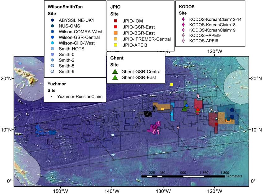
Washburn et al.                                                                                                  Macrofaunal Biodiversity Across the CCZ

                                            600–3000 km, while other locally abundant species were collected across ≤ 200 km.
                                            The vast majority of macrofaunal species are rare, have been collected only at single
                                            sites, and may have restricted ranges. Major impediments to understanding baseline
                                            conditions of macrofaunal biodiversity across the CCZ include: (1) limited taxonomic
                                            description and/or barcoding of the diverse macrofauna, (2) inadequate sampling in
                                            most of the CCZ, especially within APEIs, and (3) lack of consistent sampling protocols
                                            and efficiencies.
                                            Keywords: macrofauna, deep-sea mining, biodiversity, polychaeta, manganese nodules, POC flux, species
                                            ranges, areas of particular environmental interest

INTRODUCTION                                                                    capture the full range of macrofaunal biodiversity and species
                                                                                distributions in the CCZ; (2) identify needs for additional APEIs;
The Clarion-Clipperton Zone (CCZ) is an ∼ 6 million                   km2
                                                                                and (3) identify key gaps in our knowledge of macrofaunal
abyssal region in the equatorial Pacific Ocean targeted for
                                                                                biodiversity that impede APEI evaluation and assessment of risks
polymetallic nodule mining (Wedding et al., 2013). There are
                                                                                from nodule mining to regional biodiversity.
currently 16 mineral exploration contract areas, each up to
                                                                                   For this synthesis, macrofauna are considered to be animals
75000 km2 , distributed across this region (accessed 3 January
                                                                                retained on 250 – 300 µm sieves. This size fraction contributes
20201 ). While no exploitation activities have yet taken place,
                                                                                substantially to biodiversity and ecosystem functions at the
regulations for commercial exploitation are planned by the
                                                                                abyssal seafloor (Smith et al., 2008a). The abyssal CCZ
International Seabed Authority (ISA) to be in place by 2021
                                                                                macrofauna are primarily sediment-dwelling and are numerically
(ISA, 2018). Deep-seafloor ecosystems are expected to experience
                                                                                dominated by polychaete worms, and tanaid and isopod
substantial impacts from nodule mining, with single mining
                                                                                crustaceans (Borowski and Thiel, 1998; Smith and Demopoulos,
operations potentially damaging > 1000 km2 of seafloor annually
                                                                                2003; De Smet et al., 2017; Wilson, 2017; Pasotti et al., 2021).
from direct habitat disruption, turbidity, and resedimentation
                                                                                Polychaetes in particular account for ∼35 – 65% of macrofaunal
(Smith et al., 2008c; Washburn et al., 2019). The full range of
                                                                                abundance, biomass, and species richness in nodule regions (e.g.,
seafloor impacts from nodule mining may include removal of
                                                                                Borowski and Thiel, 1998; Smith and Demopoulos, 2003; Chuar
sediment and nodule habitats, sediment compaction, seafloor
                                                                                et al., 2020). Macrofaunal community abundance in abyssal
and nodule burial, dilution of food for deposit and suspension
                                                                                nodule regions of the CCZ is relatively low compared to shallower
feeders, smothering of respiratory structures, interference with
                                                                                continental margins, and typically totals 200 – 500 individuals
photoecology, and noise pollution (Smith et al., 2008c; Washburn
                                                                                m−2 (Glover et al., 2002; Smith and Demopoulos, 2003; De Smet
et al., 2019; Drazen et al., 2020). Many ecosystem impacts
                                                                                et al., 2017). Despite low abundances, the CCZ appears to host
will be long lasting since sediment habitats will require at
                                                                                high levels of macrobenthic biodiversity (Smith et al., 2008a,b).
least many decades to recover, and natural nodule habitats
                                                                                   In this paper, we address the following questions for the
will not regenerate for millions of years (Hein et al., 2013;
                                                                                sediment macrofauna:
Vanreusel et al., 2016; Jones et al., 2017; Stratmann et al., 2018a,b;
Vonnahme et al., 2020).                                                           (1) Do abundance, species/family richness and evenness, and
    Because impacts from nodule mining may be large-scale,                            community structure vary along and across the CCZ? What
intense and persistent, the ISA in 2012 established nine areas                        are the ecological drivers of these variations?
distributed across the CCZ to be protected from seabed mining,                    (2) Do mining exploration claim areas have similar levels of
called Areas of Particular Environmental Interest (APEIs)                             species/taxon richness and evenness, and similar community
(Wedding et al., 2013). The APEIs each cover 160000 km2 and                           structure, to the proximal APEI(s)?
were designed to serve as a representative system of unmined                      (3) Are macrofaunal species ranges (based on morphology
areas to protect biodiversity and ecosystem function across the                       and/or barcoding) generally large compared to the distances
region from mining impacts (Wedding et al., 2013). Since 2012,                        between APEIs and contractor areas? What is the degree of
at least thirteen sites within the CCZ region have been studied to                    species overlap between different study locations across the
collect new seafloor biodiversity and ecosystem data. These new                       CCZ?
data enable a scientific review and synthesis to help address the                 (4) What scientific gaps hinder biodiversity and biogeographic
representativity of the APEI network for protecting biodiversity                      syntheses for the macrofauna (e.g., how well is the
across the CCZ. In this paper, we review and synthesize recent                        macrofauna known taxonomically)?
biodiversity data for sediment-dwelling macrofauna, a faunal
component characterized by high biodiversity in abyssal habitats                   Our results indicate that macrofaunal abundance, diversity,
(Smith et al., 2008a). The general goals of this synthesis are to:              and community structure vary across the CCZ, driven in part
(1) consider whether the current network of APEIs appears to                    by differences in particulate organic carbon (POC) flux to the
                                                                                seafloor. However regional macrofaunal diversity is still poorly
1
    https://www.isa.org.jm/deep-seabed-minerals-contractors                     characterized, with sampling at all studied sites still rapidly

Frontiers in Marine Science | www.frontiersin.org                           2                                       April 2021 | Volume 8 | Article 626571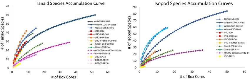
Washburn et al. Macrofaunal Biodiversity Across the CCZ
accumulating species, and major areas of the CCZ (including 250- or 300-µm sieves collected to a sediment depth of 10 cm.
most APEIs) with little or no macrofaunal sampling. Nematodes, harpacticoid copepods, and ostracods were omitted
from macrofaunal counts because these taxa are poorly retained
by 250 – 300-µm sieves and thus are generally considered to
MATERIALS AND METHODS be meiofaunal taxa (Hessler and Jumars, 1974; Dinet et al.,
1985; De Smet et al., 2017). Counts per box core at species
CCZ Macrofaunal Box-Core Data Sets and higher taxonomic levels were assembled for all samples
Data were assembled from the peer-reviewed scientific literature available from the CCZ and the broader equatorial Pacific,
and from a variety of unpublished sources through direct which included nine cores in total collected across three APEIs
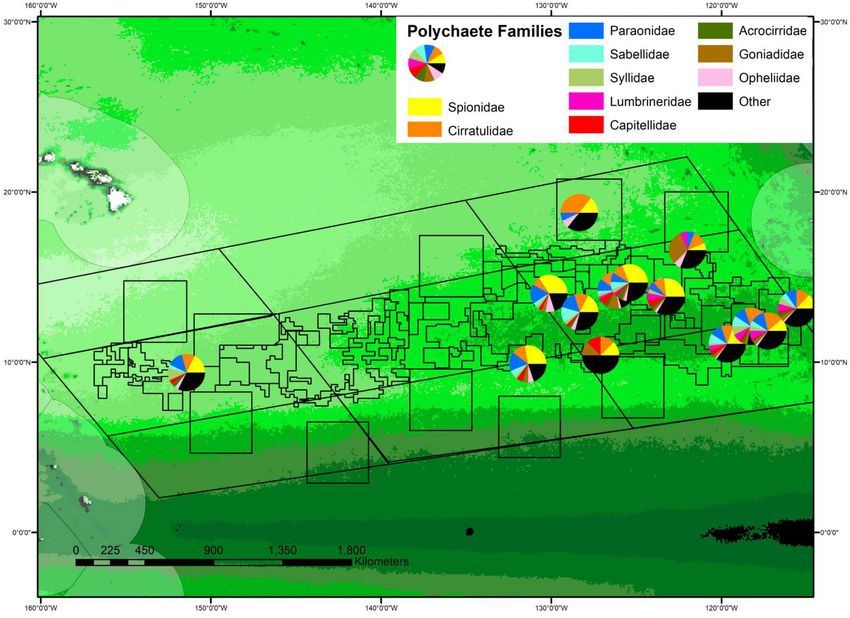
solicitation from scientists and contractors, and online posting by (Figure 1 and Table 1).
the ISA of a general data solicitation2 . The abyssal macrofaunal Data sets were obtained from eight different studies that
data assembled were collected by box corer with a sample area collected samples from eleven different contractor areas and
of 0.25 m2 (Hessler and Jumars, 1974). Data sets were restricted three APEIs (Glover et al., 2002; De Smet et al., 2017; Wilson,
to box cores because they can provide quantitative samples of 2017; Błażewicz et al., 2019b; Bonifácio et al., 2020; Chuar et al.,
adequate size for macrofaunal community studies, and there is 2020; Pasotti et al., 2021). Data sets were obtained from the
some (albeit, not complete) standardization of box-core sampling National University of Singapore (NUS), the Abyssal Biological
and processing protocols for deep-sea macrofauna (Hessler and Baseline Project (ABYSSLINE), multiple projects funded by the
Jumars, 1974; Glover et al., 2016; De Smet et al., 2017). The National Oceanic and Atmospheric Administration analyzed
box corer is a more quantitative, and less biased, sampler of by Wilson (2017) (Wilson), U.S. Joint Global Ocean Flux
infaunal macrobenthic community structure and diversity than Study (JGOFS) (Smith), Joint Programming Initiative Healthy
devices such as epibenthic sleds that collect larger, but qualitative, and Productive Seas and Oceans (JPIO) project (JPIO), the
samples. In addition, the box core has been shown to be a Belgian company Global Sea Mineral Resources (GSR) through
highly efficient sampler per unit area (Jóźwiak et al., 2020). Ghent University (Ghent), Korea Deep Ocean Study (KODOS),
For our synthesis, macrofauna consisted of animals retained on and Yuzhmorgeologiya of the Russian Federation (Yuzhmor)
(Figure 1 and Table 1). Macrofaunal data from a total of 477
2
www.isa.org.jm/workshop/deep-ccz-biodiversity-synthesis-workshop box cores were analyzed for this synthesis. Sampling sites ranged
FIGURE 1 | Map of the CCZ showing study sites from which macrofaunal box-core data were assembled for use in this study. The characteristics of the data sets
collected at these sites are presented in Tables 1, 2.
Frontiers in Marine Science | www.frontiersin.org 3 April 2021 | Volume 8 | Article 626571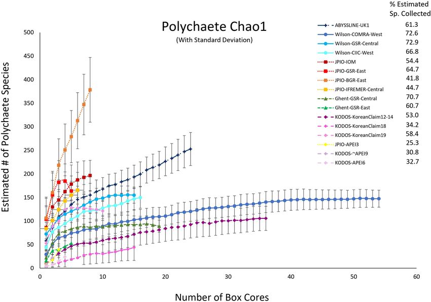
Washburn et al.                                                                                                             Macrofaunal Biodiversity Across the CCZ

TABLE 1 | Sources, numbers (#) of box cores, locations, and depths for macrofaunal box-core data used in this study.

Study         Site                     Source of Data (Name and                # of Box     Area of   Latitude (N)  Longitude (W)        Sample        Depth (m)
                                       Email or citation)                       Cores      Box Core (Decimal Deg.) (Decimal Deg.)         Dates
                                                                                           Sampled
                                                                                             (m2 )

NUS           NUS-OMS                  Tan Koh Siang –                           12        0.2267–     12.01–12.22     117.18–117.38      2015         4041–4183
                                       tmstanks@nus.edu.sg Chuar et al.,                   0.2275
                                       2020
ABYSSLINE     ABYSSLINE-UK1            Craig Smith – craigsmi@hawaii.edu         24          0.25      12.37–13.96     116.46–116.72   2013–2015       4036–4218
Wilson        Wilson-COMRA-West        Wilson, 2017                              54         0.2454      9.25–9.61      151.01–151.97   1977–1978       4842–5283
Wilson        Wilson-GSR-Central       Wilson, 2017                              15          0.25      14.62–14.71     125.37–125.46      1983        4480 – 4567
Wilson        Wilson-CIIC-West         Wilson, 2017                              16          0.25      12.91–12.98     128.28–128.37      1989        4708 – 4854
Smith         Smith-HOTS               Craig Smith – craigsmi@hawaii.edu          4          0.15      22.91–22.92     157.83–157.84      1992        4843 – 4867
                                       Glover et al., 2002
                      ◦
Smith         Smith-0                  Craig Smith – craigsmi@hawaii.edu          3          0.18       0.11–0.12      139.73–139.74      1992        4300 – 4305
                                       Glover et al., 2002
                      ◦
Smith         Smith-2                  Craig Smith – craigsmi@hawaii.edu          4          0.18       2.06–2.07      140.13–140.15      1992        4408 – 4414
                                       Glover et al., 2002
                      ◦
Smith         Smith-5                  Craig Smith – craigsmi@hawaii.edu          3          0.18       5.07–5.08      139.64–139.65      1992         4320–4446
                                       Glover et al., 2002
                      ◦
Smith         Smith-9                  Craig Smith – craigsmi@hawaii.edu          3          0.18         8.93         139.86–139.88      1992         4981–4991
                                       Glover et al., 2002
JPIO          JPIO-IOM                 Lenaick Menot –                            8          0.25      11.07–11.08     119.65–119.66      2015         4414–4434
                                       lenaick.menot@ifremer.fr
                                       Martinez Arbizu and Haeckel(eds),
                                       2015; Błażewicz et al., 2019b;
                                       Bonifácio et al., 2020
JPIO          JPIO-GSR-East            Lenaick Menot –                            5          0.25      13.84–13.86     123.23–123.25      2015         4503–4516
                                       lenaick.menot@ifremer.fr
                                       Martinez Arbizu and Haeckel(eds),
                                       2015; Błażewicz et al., 2019b;
                                       Bonifácio et al., 2020
JPIO          JPIO-BGR-East            Lenaick Menot –                            8          0.25      11.81–11.86     117.05–117.55      2015         4118–4370
                                       lenaick.menot@ifremer.fr
                                       Martinez Arbizu and Haeckel(eds),
                                       2015; Błażewicz et al., 2019b;
                                       Bonifácio et al., 2020
JPIO          JPIO-IFREMER-Central Lenaick Menot –                                6          0.25      14.04–14.05     130.13–130.14      2015         4921–4964
                                   lenaick.menot@ifremer.fr
                                   Martinez Arbizu and Haeckel(eds),
                                   2015; Błażewicz et al., 2019b;
                                   Bonifácio et al., 2020
JPIO          JPIO-APEI3               Lenaick Menot –                            3          0.25      18.77–18.80     128.34–128.36      2015         4816–4847
                                       lenaick.menot@ifremer.fr
                                       Martinez Arbizu and Haeckel(eds),
                                       2015; Błażewicz et al., 2019b;
                                       Bonifácio et al., 2020
Ghent         Ghent-GSR-Central        Ellen Pape – Ellen.Pape@ugent.be          19          0.25      14.02–14.71     125.51–125.93   2015–2017       4477–4629
                                       De Smet et al., 2017; Pasotti et al.,
                                       2021
Ghent         Ghent-GSR-East           Ellen Pape – Ellen.Pape@ugent.be           5          0.25      13.88–13.89     123.28–123.31   2015–2017       4535–4560
                                       De Smet et al., 2017
KODOS         KODOS-KoreanClaim- Se-Jong Ju – sjju@kiost.ac.kr                   15        0.23–0.25   9.85–10.52      131.33–131.93      2018         4995–5174
              2018
KODOS         KODOS-KoreanClaim- Se-Jong Ju – sjju@kiost.ac.kr                   36        0.23–0.25   10.48–10.52     131.29–131.94   2012–2014       4772–5206
              2012-14
KODOS         KODOS-KoreanClaim- Se-Jong Ju – sjju@kiost.ac.kr                   10          0.25      9.35–11.33      130.90–131.93      2019         4712–5220
              2019
KODOS         KODOS-APEI9              Se-Jong Ju – sjju@kiost.ac.kr              2        0.23–0.25   10.40–10.41     127.09–127.12      2018         4784–4792
KODOS         KODOS-APEI6              Se-Jong Ju – sjju@kiost.ac.kr              4        0.23–0.25   16.44–16.64     123.15–123.33      2018         4232–4290
Yuzhmor       Yuzhmor-RussianClaim Slava Melnik – melnikvf@ymg.ru                214       0.2175–     12.26–14.66     131.68–133.64   2010–2016       4713–5254
                                                                                            0.225
Site includes both the study and contractor area, APEI, or station name.

Frontiers in Marine Science | www.frontiersin.org                                      4                                       April 2021 | Volume 8 | Article 626571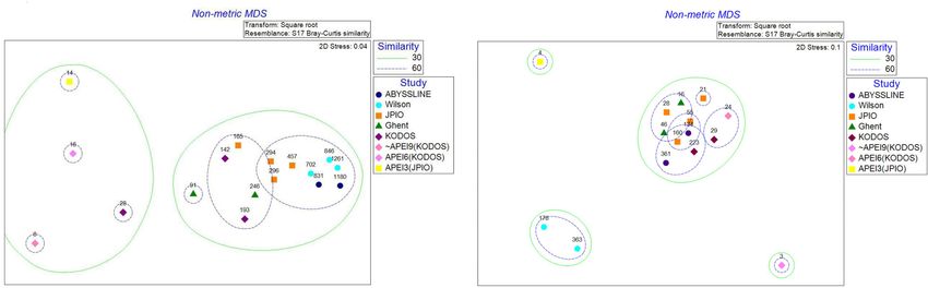
Washburn et al.                                                                                                                    Macrofaunal Biodiversity Across the CCZ

TABLE 2 | Results of linear mixed-effects models examining abundance, family richness, and species richness (taxa within a core) for polychaetes, tanaids, and isopods
within the CCZ.

Mixed-effects     Polychaete        Polychaete       Polychaete         Tanaid          Tanaid Family       Tanaid         Isopod          Isopod Family       Isopod
Models            Abundance           Family          Species         Abundance           Richness         Species       Abundance           Richness         Species
                                     Richness         Richness                                             Richness                                           Richness

Fixed Effects          4.8              3.1              1.7              46.9                52.6           32.2            18.5               10.8              7.7
Lutz POC              19.11             2.3              2.6              26.1                 42            17.7             9.2                8.8              5.2
Depth                   0                1                0               42**                32.2           35.4**         21.7**             21.3**             4.5
Nodule                 0.7               2*              0.3               0                   3.8*           1.4              0                  0               0.5
Abundance
Dissolved             13.8              2.6               0               3.6                 27.2             9              0.1                0.1              3.8
Oxygen
Random                74.8              73.1             72.6             20.7                 9.4           32.5            43.2               63.6             29.3
Effects
Best Model        POC + Depth      POC + Depth      POC + Depth      POC + Depth         All Variables   POC + Depth    POC + Depth        POC + Depth      POC + Depth
                                      + O2             + O2                                                                                 + Nodules        + Nodules
R2                     23               12.7             2.9              51.2                52.6           36.2            26.1               24.9             12.2
Random                56.6              63.5             71.4             16.4                 9.4           28.5            35.6               49.5             24.8
Effects of Best
1 0.05–0.1

* < 0.05; ** < 0.01; *** < 0.001.
Numbers represent R2 values for all four fixed effects combined, each fixed effect alone, and the random effect (study/site). The best model represents the combination
of fixed effects with the highest R2 value. KODOS, except KoreanClaim19, and Yuzhmor are excluded from these analyses due to apparent differences in sampling
efficiencies; Smith_HOTS, Smith_0o , and Smith_2o are excluded from analyses because they fall outside of the CCZ. Asterisks denote variables with significant differences
in ANOVA at the p-levels indicated below table.

in depth from ∼ 4000 – 5300 m and were collected between                                   In addition, the thousands of sediment macrofaunal species
        ◦                    ◦
0 – 23 N and 116 –158 W (data sources and shorthand                                     in the CCZ are mostly undescribed (Glover et al., 2002; Smith
names for data sets are given in Table 1). Macrofaunal data                             et al., 2008a,b; Glover et al., 2018; Błażewicz et al., 2019b;
were compiled for each research group at the site level, i.e.,                          Jakiel et al., 2019), research programs use different taxonomists
within a contract area or APEI (Figure 1 and Table 1). Most                             with different morphological reference collections to resolve
studies differentiated only a subset of macrofaunal taxa (i.e.,                         species, and some programs have combined morpho-taxonomy
polychaetes, tanaids, and isopods) to the species level; however,                       with DNA barcoding (Supplementary Table 1). Since reference
NUS data were resolved only to the family level and Yuzhmor                             collections have not been intercalibrated across all research
data to the class level (Supplementary Table 1). All studies used                       programs and only a small proportion of macrofaunal species
a 0.25 m2 box corer although some removed small subsamples                              from the CCZ have been DNA barcoded or formally described,
for other analyses (Table 1). Abundance data for all box-core                           we conducted between-site species-level comparisons primarily
samples were normalized to 1 m2 . All studies used 300-µm sieves                        within research programs to assure consistency in sampling
except for NUS, which used 250-µm. Sampling years ranged from                           protocols and species-level determinations. However, within one
1977 to 2019 (Table 1).                                                                 data set (KODOS), box cores collected on different cruises (2012–
                                                                                        2014, 2018, and 2019) appear to have different sampling biases,
                                                                                        with the percentage of polychaetes resolvable to species level,
The Comparability of Box-Core Data Sets                                                 polychaete abundances, and species/family accumulation curves
There was substantial variability among “quantitative” box-core                         exhibiting large differences among sampling times; we thus
data sets in taxa counted and taxonomic resolution obtained. In                         analyzed the KODOS samples as three different data sets. It
addition, box-core samples were collected by different research                         should be noted that the box-core data sets contributed by Wilson
programs (Table 1) using a range of box-core designs, box-                              (Wilson), Smith (ABYSSLINE and Smith), and Tan (NUS) were
core deployment protocols (e.g., lowering speed, stern vs. side                         collected and processed with similar protocols [first described in
A-frame, etc.), and sample-washing procedures (e.g., sieve size,                        Hessler and Jumars (1974), and more recently in Glover et al.
washing-water temperature, on-board vs. in-laboratory sieving,                          (2016)] by lead personnel trained in a single laboratory (that of
etc.), all of which may influence sampling efficiency and the                           R. R. Hessler), so these samples were considered to be a single
ability to resolve macrofauna at the species level (Glover                              Wilson–Smith–Tan data set for abundance analyses.
et al., 2016). Most macrofaunal box-core data sets distinguished                           To allow diversity comparisons across data sets, we analyzed
polychaetes, tanaids, and isopods to morphospecies. However,                            patterns at the family level after harmonizing the family
taxonomic and systematic resolution differed among these                                level taxonomy using the World Register of Marine Species
groups (e.g., many tanaid species were not classified into                              (WoRMS3 ).
families), and only one study (ABYSSLINE) distinguished species
for all macrofauna collected (Supplementary Table 1).                                   3
                                                                                            www.marinespecies.org

Frontiers in Marine Science | www.frontiersin.org                                   5                                                 April 2021 | Volume 8 | Article 626571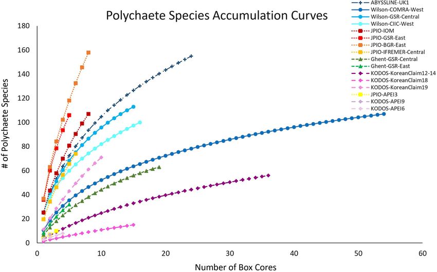
Washburn et al.                                                                                             Macrofaunal Biodiversity Across the CCZ

Analytical Methods                                                       the number of species found in more than one contractor
Analyses of the Comparability of Data Sets                               area was calculated within studies for “working species,” and
Macrofaunal patterns across sites were first explored with               across studies for “described species.” “Working species” (i.e.,
regression analyses between macrofaunal abundances and                   “morphospecies”) have been differentiated by a taxonomist but
individual environmental parameters, in particular POC flux,             have not been assigned to a described species (i.e., they are
nodule abundance estimated from the ISA (2010) Geological                likely new to science); working species are assigned numbers or
Model, and ocean depth. Direct deep POC flux measurements                letters that vary across taxonomists and studies. The number
(e.g., from sediment traps) are not available from the study             of species shared between sites was explored in the JPIO data
sites considered here. Thus, to explore the relationship between         set (Błażewicz et al., 2019b; Bonifácio et al., 2020) using UpSet
seafloor particulate organic carbon (POC) flux and polychaete            plots generated in R (Conway et al., 2017). UpSet is a technique
abundance, we estimated seafloor POC flux for sampling                   which visualizes data intersections and sizes of these intersections
localities using the Lutz et al. (2007) POC-flux model and the           (Conway et al., 2017).
data set created by Lutz et al. (2007), which was calculated for             Linear Mixed-Effects Modeling, ‘lmer,’ in R, was used
the period 1997 – 2004, an interval near the middle of the               to explore which environmental variables best explained
range in sampling times (1977–2019) of box cores used in this            macrofaunal abundance and taxonomic richness across
study; we call these estimates “Lutz POC flux.” The Lutz et al.          individual box cores (Bates et al., 2015). Sample depth, Lutz
(2007) POC flux model is trained with sediment-trap data from            seafloor POC flux (Lutz et al., 2007), nodule abundance (kg/m2 )
the CCZ and the equatorial Pacific region generally, and yields          (Morgan, 2012), bottom-water oxygen concentration, bottom-
results consistent with diagenetic modeling of seafloor POC in           water salinity, bottom-water temperature, bottom-water nitrate,
the CCZ (Volz et al., 2018). This model has been widely used             phosphate, and silicate concentrations (all downloaded from
to evaluate regional patterns of seafloor POC flux in the deep           World Ocean Atlas 20184 ; Washburn et al., 2021), bottom
sea (e.g., Sweetman et al., 2017; Snelgrove et al., 2018). Type II       slope (largest change in elevation between a cell and its eight
regression analyses of polychaete abundance versus Lutz POC              neighbors), broad-scale bathymetric position index (BBPI; with
flux were performed using linear and exponential functions in            an inner radius of 100 km and outer radius of 10000 km) and
Excel, and the function ‘lmodel2’ (Legendre, 2018) in R. The             fine-scale bathymetric position index (FBPI, with an inner radius
functionality (either linear or exponential) with the highest R2         of 10 km and outer radius of 100 km) (McQuaid et al., 2020) were
was selected, and ordinary least squares (OLS) regressions were          obtained for each box-core sample location. Since environmental
used for all studies since they produced the best fit to the data.       data were not available for many individual locations and several
Linear mixed-effects modeling, ‘lmer’ (Bates et al., 2015), in R,        studies, and to ensure data were consistent across studies,
with “POC flux” as the fixed effect and “Research Program” as            data for all environmental variables (except depth, which was
the random effect was used to explore the amount of variation            provided for each sample) were extracted for each box-core
explained by POC flux versus study in polychaete abundance. If           location from interpolated rasters in ArcGis (see Washburn
studies had different sampling efficiencies, we would expect that        et al., 2021). Environmental variables were standardized, and
the “Research Program” effect would explain a relatively high            abundance/richness data were log-transformed to facilitate
proportion of the variance.                                              linearity in the relationship between abundance/richness
                                                                         and environmental variables. If the relationship between an
Analyses of Macrofaunal Abundance/Diversity,                             environmental variable and taxon abundance or richness did not
Environmental Drivers, and Community Structure                           appear linear (e.g., appearing parabolic in many cases), a second-
Biodiversity patterns were further explored with species and             order relationship was examined. A linear mixed-effect model
family accumulation curves, Chao 1 species richness estimators,          was then created with abundance or taxon richness per core as
rarefaction, and Pielou’s evenness, as described in Magurran             the dependent variable, the standardized environmental variables
(2004) using EstimateS (Colwell, 2013), R (Venables et al., 2019),       set as fixed-effect explanatory variables, and site as the random-
or PRIMER 7 (Clarke and Gorley, 2015). Rarefaction curves                effect variable. Correlations among environmental variables were
with 95% confidence limits were calculated in EstimateS for              explored by calculating the variance inflation factors (VIF) in
each site by pooling box-core samples within a site. Species             the ‘car’ package (Fox et al., 2020) and any variables with scores
accumulation curves and Chao 1 richness were calculated using            near or above 10 were removed (Montgomery and Peck, 1992).
100 permutations and the UGE index (Ugland et al., 2003) in              Studies were removed from the model if they appeared to have
EstimateS for each site using box cores as replicates. Pielou’s          skewed residuals, and models with all possible combinations of
species and family evenness were calculated in PRIMER 7 for              variables were examined using ‘dredge’ in the ‘MuMIn’ package
each box core and then averaged within a site. The number                (Barton, 2020). Exploratory analyses found that the majority of
of species at each site with abundances of 1 or 2 individuals            variables explained less than 1% of the variation in abundances
(singletons or doubletons) was calculated and compared to the            or richness, so models were refined to include only the variables
total number of species found within each site. A similarity             explaining > 5% of the variance, i.e., depth, Lutz POC flux,
percentages (SIMPER) analysis was used to examine community              nodule abundance, and bottom-water oxygen concentration.
similarity within study sites while an analysis of similarity            Relationships between environmental variables and abundance
(ANOSIM) test was used to examine community differences
among sites within a study (Clarke and Gorley, 2015). Finally,           4
                                                                             www.nodc.noaa.gov/OC5/woa18/

Frontiers in Marine Science | www.frontiersin.org                    6                                         April 2021 | Volume 8 | Article 626571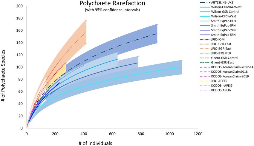
Washburn et al.                                                                                                               Macrofaunal Biodiversity Across the CCZ

or richness in the best models, measured by AIC and R2 values,                        would be expected if they were from the same statistical
were explored further with ANOVAs and regression plots                                population, with a number of data sets falling largely above or
(Zuur et al., 2009).                                                                  essentially entirely below the curve. This suggests that individual
    Community composition for polychaetes at the species level,                       data sets may have different relationships between POC flux and
and for other taxa at the family level, was compared among                            polychaete abundance, as might be expected if sampling protocols
sites using non-metric multidimensional scaling on square-root                        (and sampling efficiency) varied among research programs.
transformed abundances/m2 in PRIMER 7. SIMPER analysis                                Furthermore, in the linear mixed effect model including all data
was then used to explore which taxa were responsible for                              with research program as the random effect and POC flux as the
similarities/differences within and among studies.                                    fixed effect, the research program effect explained 51% of the
                                                                                      variation while POC flux explained 19% (p < 0.0001). This is
                                                                                      also consistent with the hypothesis that sampling efficiency varied
RESULTS                                                                               among research programs.
                                                                                         We then conducted regressions of POC flux versus polychaete
The Comparability of Box-Core Data Sets                                               abundance for individual research programs, i.e., studies that
Because polychaetes typically constituted > 50% of macrofaunal                        were conducted by investigators trained within the same
abundance, and polychaete abundance was tabulated in all                              laboratory and thus expected to use similar sampling protocols.
the box-core data sets, polychaete abundance was used to                              The Wilson–Smith–Tan and JPIO studies exhibited positive
explore comparability (e.g., sampling efficiency) across research                     exponential relationships with high R2 values (>0.7), while all
programs. Based on previous abyssal studies of the relationships                      other studies, except for KODOS, showed positive but weaker
between seafloor POC flux and macrofaunal abundance (Glover                           exponential relationships to Lutz POC flux (Figure 2). The
et al., 2002; Smith et al., 2008a; Wei et al., 2010), it was                          KODOS data showed a negative exponential relationship to
expected that polychaete abundance across the CCZ would                               POC flux, driven largely by relatively low values in box cores
exhibit a positive relationship (exponential or linear) with                          collected prior to 2019 (Figure 2), potentially due to differences in
estimated annual seafloor POC flux (Lutz et al., 2007).                               sampling protocols, sea states, and/or seasonal/temporal trends
Abundances per box core spanned an order of magnitude                                 in the KODOS area. The Wilson–Smith–Tan data covered the
across studies (Supplementary Figure 1), likely in part due to                        broadest ranges of longitude, latitude and POC fluxes while
variations in POC flux.                                                               JPIO data covered the second broadest ranges of these variables
   When box-core samples were pooled across all studies,                              (Table 1), providing robust support for the importance of POC
polychaete abundance was exponentially related to POC flux                            flux as an ecosystem driver across the CCZ (cf. Smith et al.,
(Figure 2), with 20% of the variation explained. However,                             2008a; Wedding et al., 2013; Bonifácio et al., 2020). Due to the
the data from individual sampling programs were not evenly                            differing relationships between polychaete abundance and POC
distributed above and below the overall regression curve, as                          flux across studies, we hypothesized that different studies had

  FIGURE 2 | Polychaete abundance in individual box cores versus Lutz POC flux. Curves are Type II regressions conducted in R, with regression equations, R2
  values, and p levels of regressions indicated. The bold red line is the exponential regression for all sampling programs combined. Regression lines for data sets
  match the colors of their symbols in the upper left. The pink regression line represents all KODOS data, while yellow diamonds represent KODOS samples collected
  in 2019. This figure does not show data points for Smith-0, Smith-2, or Smith-5 (which are included in the regressions/curves) as they have much larger POC fluxes
  and abundances than all other sites making observations of trends for other studies difficult.

Frontiers in Marine Science | www.frontiersin.org                                 7                                              April 2021 | Volume 8 | Article 626571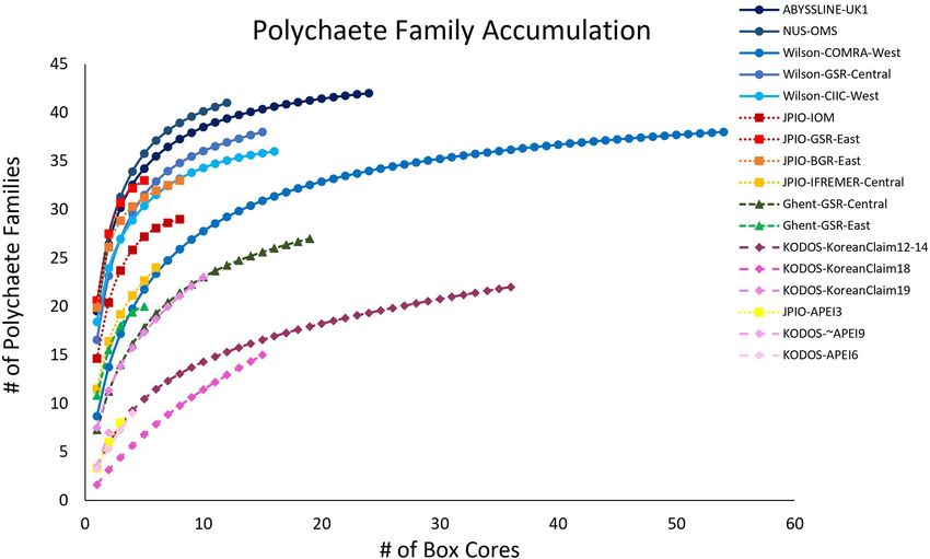
Washburn et al.                                                                                                          Macrofaunal Biodiversity Across the CCZ

different sampling efficiencies and were not directly comparable,                  slope (i.e., slope, BBPI, FBPI) explained little to no variation
so further analyses were performed separately on data sets from                    in polychaete abundances and were thus removed. ANOVA
individual research programs.                                                      found that only POC flux had a nearly significant p-value
                                                                                   (p = 0.06). Fixed effects (i.e., environmental variables) in the
                                                                                   model explained 23% of variation in polychaete abundance when
Question 1: Do Abundance,                                                          KODOS from 2012 – 2018 and Yuzhmor data (i.e., data sets with
Species/Family Richness and Evenness,                                              very different apparent sampling efficiencies) were excluded. This
and Community Structure, Vary Along                                                was almost solely due to POC flux, since the model containing
and Across the CCZ? What Are the                                                   POC flux alone explained 19% of the variation. Neither depth
                                                                                   nor nodule abundance explained substantial variation while the
Ecological Drivers of These Variations?                                            inclusion of oxygen concentration actually decreased the R2 of
Abundance Patterns                                                                 the model (Table 2). It is noteworthy that random (study/site)
Regional patterns of polychaete abundance                                          effects explained three times as much variability in polychaete
Polychaete abundance showed strong variations along and across                     abundance (57%) as the fixed effects, highlighting that there
the CCZ, including within data sets (e.g., the Wilson–Smith–                       are large differences among sampling programs and/or sites not
Tan data in blue and the JPIO data in yellow) (Supplementary                       explained by the current set of environmental variables; these
Figure 2). Many of the between-site differences are clearly                        differences are likely caused, at least in part, by differences in
statistically significant, as indicated by the small size of within-               sampling efficiency among studies.
site standard errors compared to between-site differences. As
noted above (Figure 2), regression analyses indicate that these                    Regional patterns of tanaid and isopod abundance
variations in polychaete abundance across the region are strongly                  Regression relationships between tanaid and isopod abundances
related to Lutz POC flux (Lutz et al., 2007), supporting the use                   and Lutz POC flux were similar to those for polychaete
of seafloor POC flux to divide the CCZ management area into                        abundance. POC flux explained 57 and 47% of variability in
ecological subregions (Wedding et al., 2013).                                      tanaid abundances for the Wilson–Smith–Tan and JPIO data
    Lutz POC flux explained >70% of the variability in polychaete                  sets, respectively, and 26% of tanaid variability for all studies
abundances across the CCZ for two studies and 20% of                               combined. POC flux explained 21 and 17% of variability in
variability for all studies combined. Regional nodule abundance,                   isopod abundances for the Wilson–Smith–Tan and JPIO data sets,
when assessed individually with Type II regression, exhibited                      respectively, and only 7% of isopod variability for all studies
little relationship with polychaete abundance for all data sets                    combined (Supplementary Figures 3A, 4A). Nodule abundance
combined, but explained 38 and 48% of variation in the Wilson–                     explained approximately 10% or less of the variation for both
Smith–Tan and JPIO data sets, respectively (Figure 3, Smith-0,                     tanaid and isopod abundances for all data sets combined as
Smith-2, and Smith-5 not shown). The relationships between                         well as for each data set independently, except JPIO; there,
depth and polychaete abundance were generally negative,                            nodule abundance explained 27 and 33% of tanaid and isopod
explaining 25% of variability among polychaete abundances                          abundances, respectively. However, unlike all other studies, the
when all data sets were combined, and 41 and 35% of                                relationships between nodule abundance and polychaete, tanaid,
abundances for the Wilson-Smith-Tan and JPIO data sets,                            and isopod abundances in JPIO samples were best described
respectively (Figure 3).                                                           by second-order polynomial functions with maximum animal
    We also explored the relationship between average polychaete                   abundances at intermediate nodule abundances (Supplementary
abundance at all sites sampled across the region (Figure 1)                        Figures 3B, 4B).
versus Lutz POC flux to the seafloor, depth, bottom-water oxygen                      Depth explained 31% of variability of tanaid abundances
concentration, nodule abundance, and measures of seafloor                          for all data sets combined and 39 and 47% of abundances for
slope using linear mixed-effects models. Measures of seafloor                      the Wilson–Smith–Tan and JPIO data sets, respectively. Depth

  FIGURE 3 | (A) Nodule abundance and (B) depth versus polychaete abundance in the Wilson–Smith–Tan (blue) and JPIO (yellow) data sets. Lines shown are Type II
  regressions conducted in R. All regressions are highly statistically significant (p < 0.0001).

Frontiers in Marine Science | www.frontiersin.org                              8                                            April 2021 | Volume 8 | Article 626571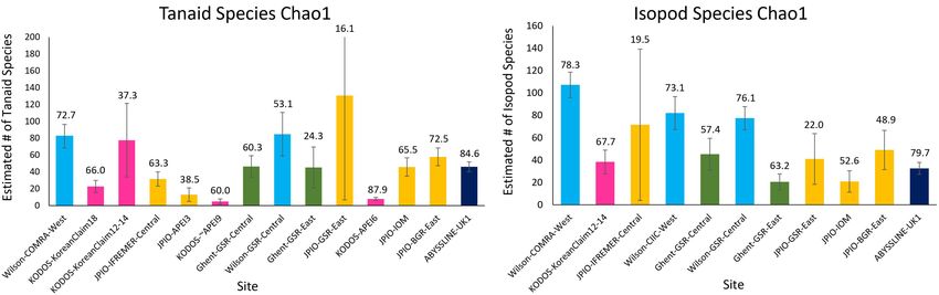
Washburn et al.                                                                                                            Macrofaunal Biodiversity Across the CCZ

exhibited little relationship with isopod abundances for all data                   of the model when depth was left in, suggesting that half of the
sets combined. Depth explained 27, 43, and 47% of variability                       variability related to depth may be caused by covarying POC
of isopod abundances for the Wilson–Smith–Tan, JPIO, and                            flux. Nodule abundance explained 0% of the variability for either
Ghent data sets, respectively. However, unlike polychaetes and                      tanaid or isopod abundance (Table 2).
tanaids, regression relationships for isopod abundances were
best represented by second-order polynomial functions with                          Biodiversity Patterns at the Species Level
maximum abundances at intermediate depths for Wilson–Smith–                         Polychaetes
Tan, but with minimum abundances at intermediate depths                             All sites with species-level, box-core data for polychaetes
for JPIO and Ghent. Measures of slope explained little to                           exhibited rising species accumulation curves, in many cases with
no variation in tanaid or isopod abundances (Supplementary                          steep slopes and with none approaching a plateau (Figure 4).
Figures 3C, 4C).                                                                    These curves indicate that polychaete species richness at all
   Overall, these regression relationships suggest that on regional                 sites remains under-sampled, i.e., species are still accumulating
scales across the CCZ, POC flux, and to lesser degrees nodule                       rapidly and additional sampling at any site will collect previously
abundance and depth, are likely to be important drivers of tanaid                   unsampled species, even when large numbers of box cores have
and isopod abundances. The differences in these relationships                       already been collected (e.g., >50 at COMRA-West; Table 1). The
among studies and the lack of relationships to POC flux, nodule                     rapidly rising curves reflect the fact that many/most species at
abundance, and depth for the Ghent, KODOS, and Yuzhmor data                         each site are rare; >49% of species were singletons or doubletons,
sets further suggest differences in sampling efficiencies among                     i.e., represented by only one or two individuals, in the pooled
studies. These differences may also be due in part to the narrow                    samples from any site (Figure 5). Within internally consistent
range of variation among explanatory variables in the above data                    data sets (e.g., within the Wilson and within the JPIO data sets),
sets due to their limited geographical extents.                                     there are substantial between-site differences in the slopes and
   Linear mixed-effects models for both tanaid and isopod                           apparent asymptotes of species accumulation curves (Figure 4).
abundance indicated that environmental variables were                                   Because species were still accumulating at all sites, the Chao
important, with fixed effects explaining over 50% of the                            1 statistic (Figure 6) was used to estimate the total number
variability in tanaid abundances and 25% for isopod abundances                      of species expected to be collected at each site (Magurran,
in the best models. ANOVA indicated that depth was significant                      2004). Chao 1 estimates range from ∼25 to ∼370 species, with
for both tanaids (p = 0.004) and isopods (p = 0.006). The                           all the relatively well-sampled sites estimated to have > 100
inclusion of oxygen and nodule abundance in either model                            species of polychaetes. Estimated total species richness at all
decreased its ability to explain variations in abundances. For                      sites substantially exceeds the number of species collected, i.e.,
both tanaids and isopods, depth alone explained nearly all the                      only 25 – 73% of estimated polychaete species richness has been
variability attributed to fixed effects. POC flux explained roughly                 recovered at any site (Supplementary Figure 5). It is important
half of the variability in either model (tanaids ∼25%, isopods                      to note that for many sites (ABYSSLINE-UK1, Wilson-CIIC-
∼10%). Removal of POC flux did not appear to affect the quality                     West, all five JPIO sites), the Chao 1 curves are increasing

  FIGURE 4 | Mean polychaete species accumulation as a function of number of box-core samples (UGE plot from EstimateS, 100 permutations) at different sites in
  the CCZ region. Note that KODOS-KoreanClaim data come from a single site sampled in different years. Data sets that are considered to have been sampled with
  similar protocols and to have used a consistent taxonomy are indicated by similar symbols.

Frontiers in Marine Science | www.frontiersin.org                               9                                             April 2021 | Volume 8 | Article 626571
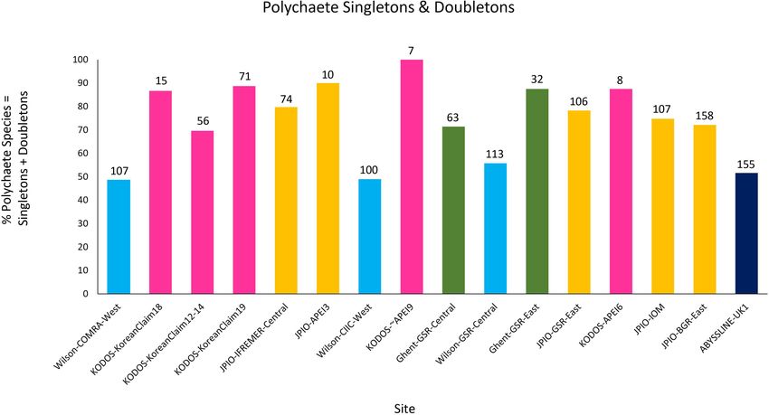
Washburn et al.                                                                                                                Macrofaunal Biodiversity Across the CCZ

  FIGURE 5 | Percentage of total polychaete species represented by singletons + doubletons in pooled collections from each site and study. The total number of
  polychaete species collected in each data set is indicated at the top of each bar. Note that KODOS-KoreanClaim data come from a single site sampled in different
  years, and potentially with different sampling efficiencies. Data sets considered to have been sampled with similar protocols and to have used a consistent taxonomy
  are indicated by similar colors.

  FIGURE 6 | Chao 1 (+SD) estimates of polychaete species richness as a function of number of box cores collected at 16 sites across the CCZ region. Note that
  KODOS-KoreanClaim data come from a single site sampled in different years. Data sets considered to have been sampled with similar protocols and to have used a
  consistent taxonomy are indicated by similar symbols.

rapidly with additional box cores (Figure 6) suggesting that at                        JPIO data (based on morphological and molecular differentiation
these sites, estimated species richness will increase substantially                    of species) indicate substantial variability in species richness
with additional sampling (i.e., the current Chao 1 number is an                        across sites (Supplementary Figure 5), which appears to be
underestimate). Species diversity (including richness) can only be                     driven by differences in POC flux and nodule abundance
directly compared between those sites with a common polychaete                         (Bonifácio et al., 2020).
taxonomy (i.e., internally consistent species differentiation),                           Individual-based species rarefaction curves for all sites exhibit
and only one internally consistent box-core data set, JPIO,                            similar initial slopes (with overlapping 95% confidence limits)
has sampled > 3 sites (n = 5) across a substantial range                               suggesting similar, high levels of species evenness across sites
(1400 km) of the CCZ (Figure 1; Bonifácio et al., 2020). The                           (Supplementary Figure 6). However, rarefaction diversity at

Frontiers in Marine Science | www.frontiersin.org                                 10                                              April 2021 | Volume 8 | Article 626571
Washburn et al.                                                                                                             Macrofaunal Biodiversity Across the CCZ

higher numbers of individuals, i.e., toward the right ends of                         set, with IOM, BGR-East, and GSR-East clustered together and
curves and at Es(130) , exhibit significant variability across sites                  different from Ifremer, which had lower abundances per sample
within data sets (Figure 7 and Supplementary Figure 6). These                         than the other three sites (Supplementary Figure 8).
between-site differences in rarefaction diversity were not strongly
related to POC flux (Supplementary Figure 6), in agreement                            Tanaids and isopods
with the findings of Bonifácio et al. (2020) for the JPIO data set.                   Rapid rates of species accumulation were observed across all sites
    Mean Pielou Evenness J’, calculated at the box-core level,                        for tanaid and isopod crustaceans, as for polychaetes, indicating
was generally high (near 1.0) and showed little variation across                      that these crustacean assemblages remain poorly sampled
sites, except that the Wilson-CIIC-West site value was unusually                      (Figure 8). As for polychaetes, large proportions of the species
low (∼0.9) (Supplementary Figure 7). Overall, this result                             at all sites (>45%) were represented by singletons + doubletons,
is consistent with the similarity of initial slopes of species                        and a substantial percentage of Chao-1 estimated species richness
rarefactions curves in Figure 7.                                                      remained uncollected (>15%), indicating that these assemblages
    No environmental variables in the linear mixed-effects model                      are incompletely sampled, even with >50 box cores (Wilson-
for polychaete species richness per core were significant in                          COMRA-West). Within data sets, there was some heterogeneity
ANOVA. The fixed effects (POC flux, Depth, O2 , and nodule                            between sites in accumulation curves and estimated species
abundance) explained less than 5% of species richness. On the                         richness (Figures 8, 9). Estimated total species richness at most
other hand, the random variable explained over 70% of richness                        sites substantially exceeds the number of species collected for
differences (Table 2), suggesting that differences in sampling                        both tanaids and isopods with only 16–85% of estimated tanaid
efficiency and taxonomy among research programs may have                              species richness, and 20–80% of isopod richness, recovered at
contributed to differences in species richness among studies.                         any site (Figure 9). Unlike polychaetes, individual-based species
    The similarity of polychaete communities among box cores                          rarefaction curves for tanaids exhibit similar curves across most
from single studies, measured by SIMPER, ranged from 0 to                             sites. Only one data set, Wilson, collected more than 30 isopods
49%. ANOSIM tests found communities differed significantly                            at two or more sites, and rarefaction curves for these three sites
among the three sites in the Wilson data set and the five sites                       were similar as well (Supplementary Figure 9).
in the JPIO data set. Generally, communities at sites further                             Unlike polychaete species richness, the fixed (environmental)
away were more different. However, evenness and the proportion                        effects in the best mixed effects model for tanaid species
of species represented as singletons are high, which means                            richness explained over 35% of variation. ANOVA results for
that samples with few individuals are likely to be dissimilar to                      this model show a significant difference for depth, and nearly
other samples. For the Wilson data set, communities at GSR-                           all the variation explained in the model was attributed to
Central and CIIC-West clustered together vs. COMRA-West,                              depth. POC flux explained roughly half of the variation in
but abundances were also lower in COMRA-West vs. the other                            tanaid richness as depth, suggesting that half of the apparent
sites. Samples from COMRA-West appeared to have decreasing                            influence of depth on tanaid richness is due to POC flux.
similarity with decreasing abundance (Supplementary Figure 8).                        Nodule abundance explained less than 2% of variation. The fixed
A similar trend was observed in samples from the JPIO data                            effects in the mixed effects model for isopod species richness

  FIGURE 7 | Individual-based polychaete species rarefaction curves by site. Envelopes indicate 95% confidence limits for curves. Note that the KODOS-KoreanClaim
  data come from a single site sampled in different years. Data sets considered to have been sampled with similar protocols and to have used a consistent taxonomy,
  are indicated by similar line types.

Frontiers in Marine Science | www.frontiersin.org                                11                                            April 2021 | Volume 8 | Article 626571
Washburn et al. Macrofaunal Biodiversity Across the CCZ
FIGURE 8 | Mean (A) tanaid and (B) isopod species accumulation as a function of number of box-core samples (UGE plot from EstimateS, 100 permutations) at
different sites in the CCZ region. Note that the Korean Claim data come from a single site sampled in different years. Data sets considered to have been sampled
with similar protocols and to have used a consistent taxonomy, are indicated by similar symbols.
FIGURE 9 | Chao 1 (+SD) estimate of species richness for (A) tanaid and (B) isopod assemblages at the various sites sampled across the CCZ. Numbers over bars
indicate the percentage of estimated species richness that has been collected at each site.
explained roughly 10% of variation while ANOVA results showed than sampling of many hundreds of rare, undescribed species.
no significant differences in any environmental variables for For older data sets (e.g., Wilson, 2017), we updated family
this model (Table 2). The random effect explained over 30% classifications to the current family taxonomy using WoRMS.
of variation in tanaid species richness and over 40% in isopod
species richness, again suggesting that differences in sample Polychaetes
efficiency inhibit comparisons across studies. For most sites with >10 box-core samples, polychaete family
Within study sites, community similarities at the species level accumulation curves were leveling off (Figure 10), and the
among tanaid communities, based on SIMPER, ranged from 0 – number of families collected was generally > 80% of Chao-1
24%, and from 0 – 28% among isopod communities. ANOSIM family richness estimates (Supplementary Figure 12), suggesting
analyses found communities differed significantly among all that most sites are well sampled for polychaete families. There was
study sites in the Wilson data set for both tanaids and isopods, substantial across-site variability in estimated family richness,
and in the JPIO data set for tanaids. nMDS plots separated sites both within and across sampling programs.
in the Wilson data set for isopods but not for tanaids, while A linear mixed-effects model exploring the relationship
JPIO sites were spatially separated for tanaids and isopods (with between polychaete family richness per core and four explanatory
very low abundances, Supplementary Figures 10, 11). As for environmental variables (Lutz POC flux, depth, nodule density
polychaetes, much of the dissimilarity appeared to be directly in kg/m2 , and bottom-water oxygen concentration) found that
related to samples with small numbers of individuals. fixed effects in the best model explained approximately 15% of
variation in family richness, but only nodule abundance was
Biodiversity Patterns at the Family Level statistically significant (p < 0.05) and explained only 2% of
To minimize differences in taxonomy among data sets, we also the variation. The random effect explained over 60% of the
explored patterns of diversity and community structure at the variation (Table 2). Thus, differences in sampling efficiency or
family level. Identifications at the family level are generally unmeasured environmental, or biotic, variables may be largely
standardized across taxonomists and sampling programs, and the driving differences in polychaete family richness per core among
sampling of families is usually more complete and less biased the study sites.
Frontiers in Marine Science | www.frontiersin.org 12 April 2021 | Volume 8 | Article 626571Washburn et al. Macrofaunal Biodiversity Across the CCZ
fact, only one species (Aphelochaeta sp. 2062) was found in more
than one core in APEI 3, making it impossible to characterize
macrofaunal communities from these samples. There were only
five tanaid species and two isopod species collected in APEI 3 (all
singletons) with one species of each crustacean taxon found at
additional JPIO sites.
At the polychaete family level, nMDS analyses show all three
sites inside or near APEIs as outliers in community structure
compared to sites sampled within license areas (Figure 12).
However, these differences could well be caused by the very
limited number of box cores (3 – 4) and polychaetes (Washburn et al. Macrofaunal Biodiversity Across the CCZ FIGURE 11 | Percent composition of polychaetes by family plotted on the regional map of POC flux. The percent abundance of the 10 most common families is shown, with the size of wedges of circles proportional to percent abundance. The center of each chart in the map indicates site location, with some offsets to allow all pie charts to be visible. See Supplementary Figure S2 for POC flux scale. FIGURE 12 | NMDS plots of (A) polychaete and (B) tanaid family community structure for contractor areas and in or near APEIs. Dashed lines bound sites with 30 and 60% similarity. Numbers above points represent the number of individuals collected at each site. 1500 – 2000 km (Supplementary Figure 14). However, one species for which numerous individuals (16) were collected polychaete species (Lumbrinerides cf. laubieri) represented by (Supplementary Figure 14) while there were no described many individuals (68) was identified from stations within only species of isopods. one site separated by ∼200 km. Thus, three-quarters of the described polychaetes, including one collected many times, were Distribution of “Working Species” Within Box-Core sampled from only a small geographic range (≤200 km) while Studies some commonly collected polychaete species show evidence of The JPIO study included the largest number of different sites broad geographic ranges (Supplementary Figure 14). Among and spans ∼1400 km (Figure 1), although all the JPIO sites the fourteen described species of tanaids (Błażewicz et al., 2019a; are in the eastern CCZ. Roughly 30% of working species of Jakiel et al., 2019), only one (Stenotanais arenasi) was found at polychaetes and 5 – 10% of tanaid and isopod working species in more than one study site; this was the only described tanaid the JPIO data set range over 600 – 1200 km, with four polychaete Frontiers in Marine Science | www.frontiersin.org 14 April 2021 | Volume 8 | Article 626571
Washburn et al.                                                                                                                  Macrofaunal Biodiversity Across the CCZ

and one tanaid species occurring in APEI 3 and contract areas                            to distinguish whether species typically are endemic to single
separated by 1250 – 1400 km (Figure 13). However, roughly 60%                            sites (i.e., have small ranges compared the spacing of samples
of polychaete, 80% of tanaid, and nearly 90% of isopod species                           across the region, Figure 1), or are present but not yet sampled
were found only at single sites, with 60 – 80% of species found at                       at multiple sites.
only one site as singletons (Figure 13).
   These results suggest that the ranges of some relatively
common macrofaunal species are broad, while many other                                   DISCUSSION
species, including some with high local abundance, may have
small ranges compared to the size of exploration contract areas                          Our analyses of abundance patterns of polychaetes (which
(up to 75000 km2 ) and the distance from contractor areas to                             dominate the macrofauna), tanaids and isopods strongly
the nearest APEIs (often 100s of kilometers). However, because                           suggest the hypothesis that different sampling programs have
most macrofaunal species sampled are rare, it is very difficult                          had differing sampling efficiencies for macrofauna, although

  FIGURE 13 | UpSet plots showing the intersection of sediment macrofaunal species resolved by morphological and/or molecular approaches across the five JPIO
  sites (i.e., sites with a common species-level taxonomy) for (A) polychaetes, (B) tanaids, and (C) isopods. Vertical bars on the main plots represent the number of the
  unique species in each area (indicated by dots in the bottom part of the graph) or number of species shared across sites (dots connected by lines). Bars on the left
  are the total number of morphological species and MOTUs (Molecular Operational Taxonomic Units) identified in each of the five areas.

Frontiers in Marine Science | www.frontiersin.org                                   15                                              April 2021 | Volume 8 | Article 626571
You can also read