Hydrometeor classification of quasi-vertical profiles of polarimetric radar measurements using a top-down iterative hierarchical clustering method ...
←
→
Page content transcription
If your browser does not render page correctly, please read the page content below
Atmos. Meas. Tech., 14, 1075–1098, 2021
https://doi.org/10.5194/amt-14-1075-2021
© Author(s) 2021. This work is distributed under
the Creative Commons Attribution 4.0 License.

Hydrometeor classification of quasi-vertical profiles of polarimetric
radar measurements using a top-down iterative hierarchical
clustering method
Maryna Lukach1,2 , David Dufton1,2 , Jonathan Crosier3,4 , Joshua M. Hampton1,2 , Lindsay Bennett1,2 , and
Ryan R. Neely III1,2
1 National Centre for Atmospheric Science, Leeds, United Kingdom
2 School of Earth and Environment, University of Leeds, Leeds, United Kingdom
3 National Centre for Atmospheric Science, Manchester, United Kingdom
4 Department of Earth and Environmental Sciences, University of Manchester, Manchester, United Kingdom

Correspondence: Maryna Lukach (maryna.lukach@ncas.ac.uk)

Received: 10 April 2020 – Discussion started: 20 May 2020
Revised: 19 November 2020 – Accepted: 30 November 2020 – Published: 10 February 2021

Abstract. Correct, timely and meaningful interpretation of       1   Introduction
polarimetric weather radar observations requires an accu-
rate understanding of hydrometeors and their associated mi-      The task of radar-based hydrometeor classification (HC) can
crophysical processes along with well-developed techniques       be broadly defined as the recognition of different hydrome-
that automatize their recognition in both the spatial and tem-   teor types in the atmosphere as represented by the various ob-
poral dimensions of the data. This study presents a novel        served moments collected by weather radar. In general, HC
technique for identifying different types of hydrometeors        is able to label radar signatures observed at any one time with
from quasi-vertical profiles (QVPs). In this new technique,      physical properties, and, over a period of time, the evolution
the hydrometeor types are identified as clusters belonging       of these labels can provide insight into the underlying atmo-
to a hierarchical structure. The number of different hydrom-     spheric processes. As such HC has many impactful applica-
eteor types in the data is not predefined, and the method        tions: HC simplifies the detection of the melting layer (Bal-
obtains the optimal number of clusters through a recursive       dini and Gorgucci, 2006), HC is necessary for obtaining ac-
process. The optimal clustering is then used to label the        curate estimates of precipitation quantities (Giangrande and
original data. Initial results using observations from the Na-   Ryzhkov, 2008) and HC provides critical information for im-
tional Centre for Atmospheric Science (NCAS) X-band dual-        proving modelling of physical processes in the atmosphere
polarization Doppler weather radar (NXPol) show that the         (Vivekanandan et al., 1999).
technique provides stable and consistent results. Compari-          Radar-based HC requires an extensive and accurate (i.e.
son with available airborne in situ measurements also indi-      expert) knowledge of the physical properties of both multi-
cates the value of this novel method for providing a physical    variate polarimetric observations and the hydrometeor par-
delineation of radar observations. Although this demonstra-      ticles themselves (Hall et al., 1984). Achieving an accurate
tion uses NXPol data, the technique is generally applicable      and precise radar-based HC is difficult due to the deficien-
to similar multivariate data from other radar observations.      cies (such as low spatial–temporal resolution) and inaccura-
                                                                 cies (such as attenuation) that are inevitable in all radar mea-
                                                                 surements. The process of HC is made even more difficult
                                                                 when this analysis needs to be performed during the oper-
                                                                 ational processing of the radar observations where there is a
                                                                 lack of time for expert assessment. Therefore, automatization
                                                                 of spatial and temporal analysis of multivariate polarimetric

Published by Copernicus Publications on behalf of the European Geosciences Union.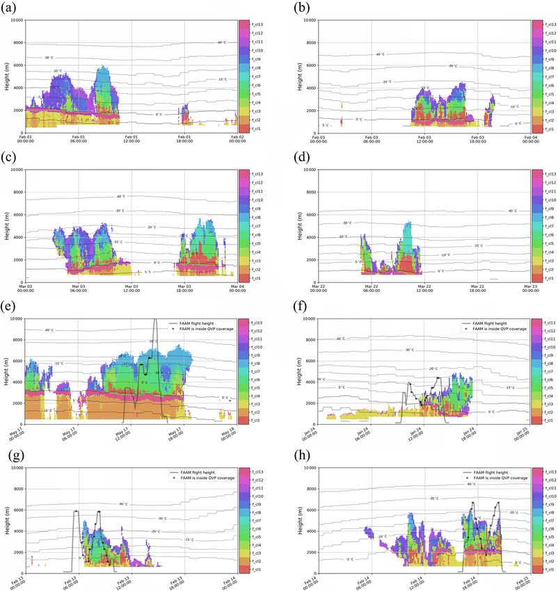
1076                      M. Lukach et al.: Hydrometeor classification of QVPs using a top-down hierarchical clustering

data is an important task for which an advanced and well-           radar signatures to possible physical properties of hydrome-
tested technique should be developed and utilized.                  teors. Thus, this approach does not impose a predefined phys-
   The development of radar-based HC started in the 1980s           ical view on the observations but provides a framework for a
and 1990s with the works of Hall et al. (1984), Hendry              more efficient physical interpretation of the properties of the
and Antar (1984), Aydin et al. (1986), Straka and Zrnić            resulting clusters of observed multivariate data in which sub-
(1993), and Straka (1996). Further refinement and develop-          tle differences and intra-cluster relations are easier to iden-
ment of automatic HC algorithms included the application            tify. In this sense, this approach inverts the procedure of ex-
of fuzzy logic (Straka et al., 2000; Liu and Chandrasekar,          isting methods. Additionally, we ask whether such an ap-
2000), machine-learning techniques (such as the identifica-         proach can be used to provide information on the temporal
tion of clusters representing data-wise similarities) (Wen et       evolution of the identified hydrometeors and reveal relation-
al., 2015; Grazioli et al., 2015; Besic et al., 2016; Ribaud et     ships between the identified classes. Such information is key
al., 2019) and neural networks (Wang et al., 2017).                 for identifying the processes that lead to high-impact weather
   Modern radar-based HC methods (Straka et al, 1996; Liu           (i.e. flooding) and improving the physical parameterizations
and Chandrasekar, 2000; Al-Sakka et al., 2013; Grazioli et          in NWP.
al., 2015; Besic et al., 2016, 2018; Bechini and Chandrasekar,         The point of this study is not to create a set of cluster
2015; Wang et al., 2017) are based on the multivariate data of      characteristics that could be applied to other datasets; rather,
polarimetric Doppler radar observations. This includes (but         the goal is to demonstrate the viability of this type of data-
is not limited to) the horizontal reflectivity factor ZH , dif-     driven methodology for creating a set of labelled clusters (i.e.
ferential reflectivity ZDR , the co-polar correlation coefficient   hydrometeor classes) based on quasi-vertical profile (QVP)
ρHV , differential phase shift on propagation 8DP , and spe-        data. As such, the comparison to in situ data and labelling
cific differential phase KDP (for definitions, see Bringi and       done as part of this study is only shown as an example of
Chandrasekar, 2001) as well as associated derived variables         how this tool can be used.
(e.g. standard deviation). Additionally, temperature and other         The existing data-driven unsupervised (Grazioli et
meteorological data, retrieved from radiosondes or numerical        al., 2015; Ribaud et al., 2019; Tiira and Moisseev, 2020)
weather prediction (NWP) models, are often utilized (Grazi-         and semi-supervised approaches (Bechini and Chandrasekar,
oli et al., 2015; Wen et al., 2015).                                2015; Besic et al., 2016; Wang et al., 2017; Roberto et
   In most existing radar-based HC methods, the multivariate        al., 2017; Besic et al., 2018) only partially provide an an-
input data are analysed per measurement voxel, and deter-           swer to the first question (Grazioli et al., 2015) and do not
mined classes are assigned to the hydrometeor types only ac-        consider the temporal evolution or dependencies between the
cording to their characteristics. Such an approach neglects         identified classes. The approach described here performs an
intra-class relationships and the temporal evolution of the         unsupervised clustering of QVPs. QVPs were first used in
identified classes. This valuable information can also be used      Kumjian et al. (2013) and Ryzhkov et al. (2016) as a way
in the labelling of the hydrometeor types and the identifica-       of constructing a substitute for a vertical profile from a scan
tion of corresponding microphysical processes. Additionally,        conducted at constant elevation, which is a typical mode of
almost all methods within the existing literature are based on      scanning for radars used in operational networks. Calculation
theoretical assumptions on the scattering properties of ob-         of the QVPs requires horizontal homogeneity of the observed
served particles and/or are only applicable for a defined (i.e.     atmospheric processes. The height vs. time format of QVPs
previously recognized) number and type of classes. Both of          represents the general structure of the storm or its evolution.
these aspects of existing HC methods are limitations. For ex-       Note that this is a novel application of the QVP data product
ample, theoretical assumptions about the scattering proper-         and the interpretation of QVP polarimetric variables differs
ties of ice-phase hydrometeors are very uncertain due to un-        from that of plan position indicator (PPI) or range height in-
known size distributions, varying dielectric properties, fall       dicator (RHI) scans due to the averaging used to construct
orientation, and their diverse and often complex geometry           them.
(Johnson et al., 2012). A predefined number of classes or hy-          The QVP input is used in this work to build a hierarchical
drometeor types is subjective and creates artificial boundaries     structure based on the identified clusters and deliver an opti-
for algorithms; therefore, subtle differences in undefined sub-     mal number of clusters based solely on internal properties of
classes are masked, which inhibits identification of the un-        the multivariate polarimetric data. The optimal clustering is
derlying microphysical processes.                                   then used to label the hydrometeor classes and to analyse the
   Thus, in this study we take a different approach and ask         temporal evolution of the labelled microphysical processes.
the following question: can a data-driven HC approach pro-             The paper is organized as follows: in Sect. 2, we intro-
vide an optimal number of classes from the observations? We         duce the clustering methods we employ, Sect. 3 contains a
define the optimal number as the lowest number of classes           description of the polarimetric radar data and their process-
representing all pronounced dissimilarities in the input data.      ing, Sect. 4 describes the iterative clustering approach, lead-
Once the optimal set of classes is identified, the burden of        ing to the development of the hierarchical structure, Sect. 5
analysis in this approach is to relate the identified clusters of   is devoted to the characterization of the clusters and their la-

Atmos. Meas. Tech., 14, 1075–1098, 2021                                              https://doi.org/10.5194/amt-14-1075-2021
M. Lukach et al.: Hydrometeor classification of QVPs using a top-down hierarchical clustering                                    1077

belling, and Sect. 6 concludes with a summary, discussion,           part of the hierarchical structure. Another advantage of the
and thoughts on further perspectives.                                top-down approach is the possibility to have more than two
                                                                     sub-clusters belonging to one parent cluster. This allows an
                                                                     optimal number of sub-clusters for each parent cluster, repre-
2     Background of employed methods                                 senting the data-driven inheritances in the resulting hierarchi-
                                                                     cal structure. Although this advantage is often not used, and
The proposed hierarchical clustering algorithm identifies the        the bottom-up methods are preferred (Grazioli et al., 2015;
optimal number of groups of data points (clusters) in a recur-       Rimbaud et al., 2019), the method presented here fully ex-
sive loop and organizes the clusters in a hierarchical structure     ploits it for the identification of an optimal number of sub-
(undirected weighted graph). The two main steps of this ap-          clusters in each iteration.
proach are the cluster identification and the optimality check.
The cluster identification is achieved after performing dimen-       2.2   Eigenvectors and principal components
sionality reduction by principal component analysis followed
by spectral clustering. The optimality check uses validity in-       Principal component analysis (PCA) is a statistical technique
dexes to identify the final set of clusters, which best classifies   mostly utilized in exploratory analysis of multivariate data. It
the provided set of data. The description of the dimensional-        extracts the most important information from the multivariate
ity reduction and clustering methods with background infor-          dataset, generating a simplified view of the original data by
mation about the validity indexes employed can be found in           dimensionality reduction.
this section directly after a short introduction to the hierar-          To reduce a dataset’s dimensionality, a set of new orthog-
chical clustering.                                                   onal, non-correlated variables called principal components is
                                                                     calculated as linear combinations of the original variables.
2.1    Hierarchical clustering                                       The first component with the largest possible variance is se-
                                                                     lected, so it best represents the diversity of the given data.
Hierarchical clustering is a type of clustering technique that       The second component is generated under the assumption
splits or combines the data through an iterative process. Un-        of orthogonality to the first component whilst also having
like “flat” clustering techniques, hierarchical clustering is not    the largest possible variance. This process is continued un-
performed in one stage; rather, it repeats the clustering pro-       til the number of principal components is equal to the num-
cess iteratively and keeps the information about each itera-         ber of original variables (d). These components are exactly
tion of clustering in a hierarchical structure. In general, for a    the eigenvectors of the correlation matrix and are employed
given set of multivariate data points, a hierarchical clustering     as a basis for a new coordinate system (Wold, 1976; Abdi
algorithm, depending on top-down or bottom-up direction,             and Williams, 2010). The first q calculated coordinates hav-
either partitions (divides) or merges (agglomerates) the data        ing satisfactory representativeness (e.g. 85 %) can be used
into groups (a set of clusters) where data points assigned to        to preserve the most important characteristics of the original
the same cluster show similarity in multivariate values (de-         data. These q principal components can replace the initial d
pending on the context, it could be, for example, having a           variables (q < d), and the original dataset, consisting of N
small distance to each other if the points are in Euclidean          measurements on d variables, is reduced to a dataset consist-
space). The direction of the process (top-down or bottom-            ing of N measurements on q principal components.
up) may be chosen and depends on the number of individual
points in the multivariate dataset and the requirements of the       2.3   Clustering method
underlying problem.
    The top-down method begins with all available data points        One of the most popular clustering methods is the k-
organized in one cluster and splits this cluster into sub-           means algorithm (Steinhaus, 1956). Through its simple in-
clusters until a certain criterion is reached or only solely         terpretability, it is often used either as a single method or as a
singleton clusters of individual points remain in the set. The       part of more computationally expensive clustering methods
bottom-up method, on the other hand, begins with all points          (e.g. Gaussian mixtures or spectral clustering). As a single
assigned to individual clusters and, at each step, merges            method, it has difficulties with non-convex clusters and is
the most similar pairs of clusters into one until all the sub-       known to perform poorly if the input variables are correlated
clusters are agglomerated into a single cluster.                     (von Luxburg, 2007). As the basis of a more complex method
    The optimal number of clusters in both approaches can            (e.g. spectral clustering), it allows a solution of non-linear
be identified using a termination criterion. The hierarchical        cluster shapes to be found (any low-dimensional manifolds
structure in the bottom-up approach needs to be completely           of high-dimensional spaces).
finished before the optimal number of clusters can be iden-             The input data herein are multidimensional and were
tified, otherwise the upper part of the tree will remain un-         found to have non-convex cluster shapes; therefore, the spec-
known. The top-down approach allows for the iterative pro-           tral clustering method was applied (Shi and Malik, 2000; Ng
cess to be stopped at any point whilst preserving the upper          et al., 2002; von Luxburg, 2007). It works by approximating

https://doi.org/10.5194/amt-14-1075-2021                                               Atmos. Meas. Tech., 14, 1075–1098, 2021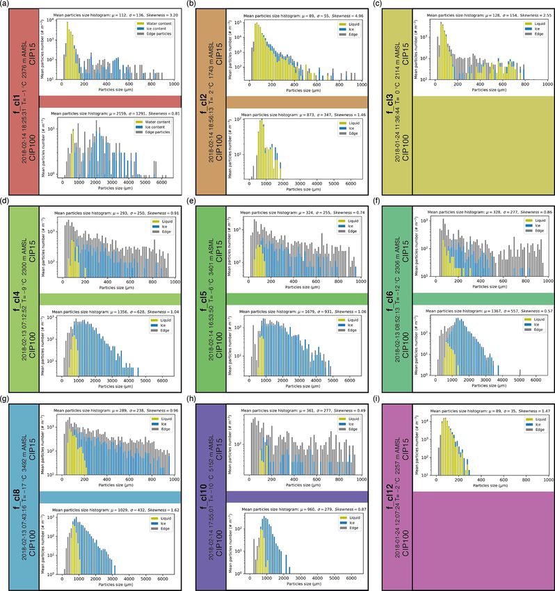
1078                          M. Lukach et al.: Hydrometeor classification of QVPs using a top-down hierarchical clustering

the problem of partitioning the nodes in a weighted graph as              is calculated, representing the WG index for the set X of
an eigenvalue problem of eigenvectors described above and                 points partitioned into K clusters (Desgraupes, 2017).
by applying the k-means algorithm to this representation in               The WG index is a measure of compactness based on
order to obtain the clusters. This work implements the Ng                 the distances between the points and the barycenters of
et al. (2002) approach and analyses the eigenvectors of the               all clusters.
normalized graph Laplacian.
   Spectral clustering has several appealing advantages. First,        2. For the BIC index, let us model each cluster ck as a
embedding the data in the eigenvector space of a weighted                 multivariate Gaussian distribution N (µk , 6k ), where
graph optimizes a natural cost function by minimizing the                 µk can be estimated
                                                                                        PK Pas the sample mean vector, and
                                                                                    1
pairwise distances between similar data points, and such                  6k = d(N−K)      k=1 i∈Ick kxi −gk k can be estimated as
an optimal embedding is analytically deducible. Secondly,                 the sample covariance matrix. Hancock (2012) showed
as was shown in von Luxburg (2007), the spectral cluster-                 that the optimal clustering is presented by maximum
ing variants arise as relaxations of graph balanced-cut prob-                           XK            nk d nk
lems. Finally, spectral clustering was shown to be more ac-               BIC (CK ) =      k=1 k
                                                                                                n log −           log 2π 6k
                                                                                                        N      2
curate than other clustering algorithms such as k-means (von                               nk − 1  1
Luxburg, 2007).                                                                         −         d − K(d + 1) log N.          (2)
                                                                                              2          2
2.4    Determining optimal number of clusters                             The BIC is an estimate of a function of the posterior
                                                                          probability of a clustering being true, under a certain
Clustering algorithms can be roughly divided into two groups              Bayesian set-up, so that a higher BIC in (2) means that
based on whether the number of clusters to be found is pre-               a clustering is considered to be more likely to be the
determined or undetermined. Spectral clustering is a rather               optimal clustering.
flexible technique in the sense that it can be used with a re-
laxation (i.e. when the number of clusters to be found is pro-
vided) or without it (when the number of clusters is deter-        3     Data and processing
mined by the multiplicity of the eigenvalue 0). As the ap-
proach chosen here is not interested in a flat partitioning of     This section presents a description of the polarimetric radar
the data (rather we want to determine hierarchical structures),    data used by the hierarchical algorithm in this study as well
the determination of the optimal number of clusters is impor-      as some details of the data preprocessing that is applied be-
tant. To identify this optimal number of clusters, two evalua-     fore the QVP calculation processing. Note that the method
tion scores are used in our method: the Wemmert–Gançarski          presented here is generally applicable with similar multivari-
(WG) index (Hämäläinen et al., 2017) and the Bayesian in-          ate data from other sources. In addition, in situ observations
formation criterion (BIC) index (Pelleg and Moore, 2000;           from the FAAM Airborne Laboratory (FAAM BAe 146) are
Hancock, 2012). The WG index was chosen as best perform-           presented in this section. These data will be used for assign-
ing according to comparison studies (Niemelä et al., 2018;         ing the labels of the hydrometeor classes to the detected clus-
Hämäläinen et al., 2017). The BIC is best for the calculation      ters or cluster groups in the radar observations.
of the posterior probability of a clustering. While the exact
                                                                   3.1    X-band radar observations
use of the indexes is described in Sect. 4, the WG and BIC
indexes can be definedas follows:                                 The polarimetric data employed to demonstrate the method
   let the dataset X = xi ∈ R d : i = 1, . . ., N have cluster-    developed in this study were collected by the NXPol radar
ing CK = {ck : k = 1, . . ., K}, (K < N ), where nk denotes        whilst it was located at the Chilbolton Atmospheric Ob-
the number of samples or points in the cluster ck , and Ick de-    servatory (CAO), part of the UK’s National Centre for At-
notes the indexes of the points in X belonging to the cluster      mospheric Science’s Atmospheric Measurement and Obser-
ck .                                                               vation Facility (AMOF), in southern England (51.145◦ N,
 1. For the WG index, let R (xi ) represent the mean of rela-      1.438◦ W) from November 2016 to May 2018 (Fig. 1).
    tive distances between the points belonging to the clus-       The NXPol is a mobile Meteor 50DX (Leonardo Germany
    ter ck and the centre of its barycentric weight gk . The       GmbH) X-band, dual-polarization, Doppler weather radar
    R (xi ) value is calculated for each point xi                  with a 2.4 m diameter antenna. The radar is a magnetron-
                                                                   based system and operates at a nominal frequency of
                    kxi − gk k                                     9.375 GHz (λ ∼ 3.2 cm). The detailed characteristics of the
      R(xi ) =                          ,
                 mink6=k 0 kxi − gk 0 k                            NXPol radar can be found in Neely et al. (2018). From the
                                                                   observations made in 2017–2018 we selected eight dates
      after that the WG index,
                                                                   with the longest precipitation events occurring within a

                 1 XK                    X                         30 km range of the radar presented on Fig. 1. The exact dates
      WGX =           k=1
                          max   0, n k −  i∈Ick
                                                R(xi )  ,   (1)    and the total number of volume scans per date can be found
                N

Atmos. Meas. Tech., 14, 1075–1098, 2021                                              https://doi.org/10.5194/amt-14-1075-2021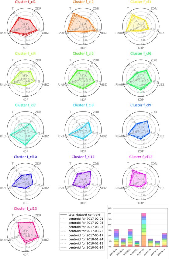
M. Lukach et al.: Hydrometeor classification of QVPs using a top-down hierarchical clustering 1079
in Table 1. Radar data selected for this study can be found Table 1. In situ data collection campaigns.
in the list of mobile X-band radar observations on the Centre
for Environmental Data Analysis (CEDA) archive (Bennett, Date FAAM Number of Number
2020). flight volume of QVP
number scans voxels
3.2 Polarimetric variables and temperature data 1 February 2017 – 243 46 656
3 February 2017 – 213 40 896
Here, we chose to use the polarimetric variables ZH [dBZ], 3 March 2017 – 213 40 896
ZDR [dB], ρHV [–], and KDP [◦ km−1 ] as well as temper- 22 March 2017 – 213 40 896
ature T [◦ C] to demonstrate the described clustering tech- 17 May 2017 C013 100 19 226
nique. The four polarimetric variables were selected as a sub- 24 January 2018 C076 196 37 632
set of all the possible variables as they provide complemen- 13 February 2018 C081 189 36 288
tary information about the observed hydrometeor properties. 14 February 2018 C082 189 36 288
Here, KDP is calculated as the linear gradient of differential
phase shift, where the phase shift has been filtered to remove
non-meteorological targets (ρHV > 0.85) and progressively
a 0.5◦ elevation angle. The use of the 20◦ PPI minimizes
smoothed using decreasing length averaging windows, and
the effects of radar beam broadening and horizontal inho-
ZH and ZDR are corrected for attenuation using the standard
mogeneity. The beam-broadening effect becomes dominant
ZPHI method (Testud et al., 2000), where α = 0.27, b = 0.78
at higher altitudes when observed by a low-elevation scan
and specific differential attenuation is 0.14 times the specific
as was shown in Ryzhkov et al. (2016). The radar beam of
horizontal attenuation. Temperature was added to the set of
1◦ opening at 20◦ elevation is about 100 m at 2 km height,
input variables following the reasoning of similar studies in
240 m at 5 km height, and reaches almost 480 m at 10 km
which either the height relative to the 0 ◦ C isotherm (Grazioli
height. The resulting profiles have 197 voxels in each QVP
et al., 2015) or the index representing the ice- or liquid-phase
at the altitudes between 0 and 10 km above mean sea level
of observed precipitation (Besic et al., 2016) was included.
(a.m.s.l.) and covering about a 30 km range from the radar. It
The full input vector used in this study can be represented as
was also shown in Ryzhkov et al. (2016) that the decrease in
follows:
ZDR from the oblate spheroidal hydrometeors at a 20◦ eleva-
x = [ZH , ZDR , ρHV , KDP , T ] . (3) tion is within the common measurement error of ZDR (0.1–
0.2 dB).
Note that this does not preclude the use of differing sets of An advantage of QVPs is that they reduce statistical errors
variables in future studies. The input data used here were pre- within the input dataset, while the height vs. time format of
processed before being utilized in the clustering algorithm: QVPs naturally represents the temporal dynamics of micro-
all range bins that were located at distances of less than physical processes observed in the radar data. To ensure the
400 m from the radar were removed from all input variables’ observations are representative of large-scale meteorological
data to reduce the influence of side lobe noise. features that may be averaged together, the QVP voxels are
The temperature data were taken from the Met Office Uni- used in the analysis only if more than 270 of the 360 az-
fied Model (UM) and interpolated onto the polar grid of the imuthal bins at the range in the PPI scan contain valid data.
radar’s observations. The original data can be found on the
CEDA archive (Met Office, 2016). Past assessments of the 3.4 In situ observations
accuracy of these temperature values suggest that the grid-
ded temperatures are within 1 ◦ C of coincident profiles mea- For the labelling of the clusters, in situ observations can be
sured by radiosondes except in the case of strong inversions used to assess any of the clusters within the hierarchical
or frontal boundaries. An example of observations from 1 d structure produced by the clustering algorithm. This allows
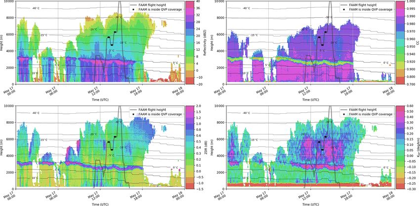
(17 May 2017) represented in the height vs. time format of for flexibility in the granularity used to examine the obser-
the QVPs of four polarimetric variables with the temperature vations. In this study, the in situ FAAM BAe 146 observa-
presented as isotherms is found in Fig. 2. Similarly, other tions are used to demonstrate the labelling and assessment of
dates from our list of cases (Table 1) are in Fig. B1. the final set of clusters. The FAAM BAe 146 is a publicly
funded research facility that, as part of the National Cen-
3.3 QVPs and thresholding tre for Atmospheric Science (NCAS), supports atmospheric
research in the UK by providing a large instrumented At-
QVPs of the input variables are obtained as the azimuthal av- mospheric Research Aircraft (ARA) and the associated ser-
erage of the data from a standard plan position indicator (PPI) vices. The ARA is a modified British Aerospace 146-301
scan at a 20◦ antenna elevation angle (Ryzhkov et al., 2016). aircraft. Further details of the FAAM BAe 146 aircraft in-
The 20◦ PPI is the highest of 10 PPIs of the volume scan- strument systems are available at https://www.faam.ac.uk/
ning strategy used by NXPol which starts the scanning from the-aircraft/instrumentation/ (last access: 25 January 2021).
https://doi.org/10.5194/amt-14-1075-2021 Atmos. Meas. Tech., 14, 1075–1098, 2021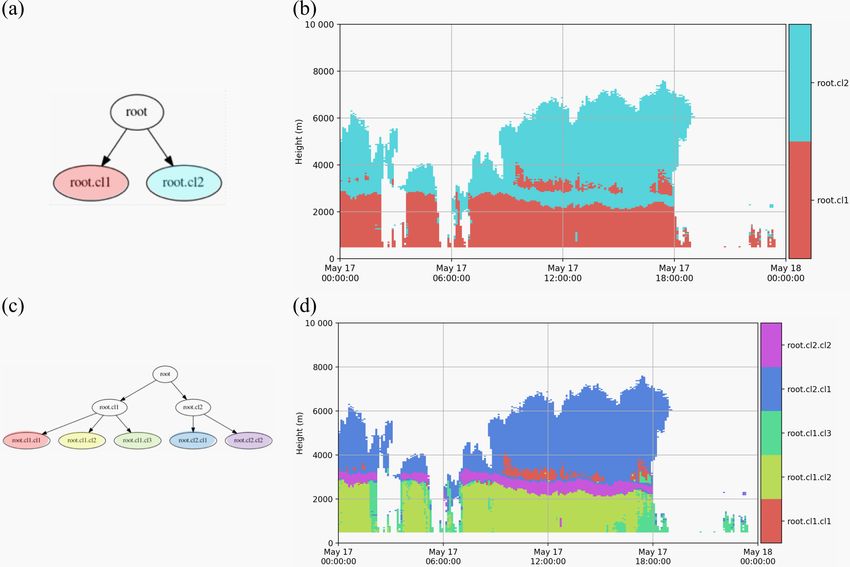
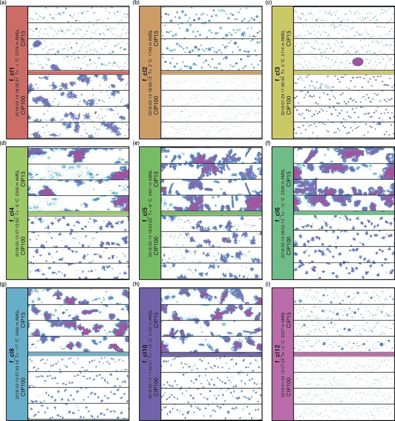
1080                        M. Lukach et al.: Hydrometeor classification of QVPs using a top-down hierarchical clustering

Figure 1. NXPol radar location at the Chilbolton Atmospheric Observatory. Circles with their centre on the radar position represent a 30, 60,
90 and 120 km range. Credit: USGS (2006).

Figure 2. The height vs. time QVPs of ZH [dBZ], ZDR [dB], ρHV [–] and KDP [◦ km−1 ] retrieved from the NXPol radar observations at
Chilbolton on 17 May 2017. Overlaid by temperature isotherms T [◦ C].

In situ data for this study come from FAAM BAe 146 flights               tured by Droplet Measurement Technologies and described
C013, C076, C081 and C082 (FAAM, 2017, 2018a, b, c),                     in Baumgardner et al. (2001). The CIPs are mounted under-
and observational data are available on the CEDA archive.                neath the aircraft wings and provide 2-bit grayscale images
The dates of the flights and their corresponding flight num-             of cloud particles as they pass through the instrument sample
bers can be found in Table 1.                                            volumes. Each CIP houses a 64-element photodiode detector,
   For the cases examined, FAAM BAe 146 was equipped                     with one CIP having an effective pixel size of 15 µm (referred
with two cloud imaging probes (CIP), which are manufac-                  to as CIP15) and the other having an effective pixel size of

Atmos. Meas. Tech., 14, 1075–1098, 2021                                                    https://doi.org/10.5194/amt-14-1075-2021
M. Lukach et al.: Hydrometeor classification of QVPs using a top-down hierarchical clustering                                  1081

100 µm (referred to as CIP100). Therefore, the CIPs provide         concentration is corrected for out-of-focus effects (Korolev,
images of particles in size ranges from 7.5 to 952.5 µm for         2007). This out-of-focus correction is not applied to the “ir-
CIP15 and from 50 to 6350 µm for CIP100. All probes have            regular” or “edge” images, as there is no evidence to show
“Korolev” anti-shatter tips – the width of which is 70 mm for       that this is an appropriate correction to make. For two key
the CIP100 and 40 mm for the CIP15.                                 reasons, no attempts have been made to classify particle im-
   Particle size distributions are calculated based on CIP data     ages. (1) The larger particles, which have the greatest influ-
where particle size is defined as being the maximum recorded        ence on the polarimetric properties, are poorly sampled by
length in either the axis of the detector array (X) or along the    the CIPs. (2) A recent study by O’Shea et al. (2020) suggests
direction of motion (Y ). All particles with inter-arrival times    that existing procedures to classify particle images using the
< 10−6 s are rejected as indicative of shattering, as in Field      CIP can lead to inaccurate results due to the effects of diffrac-
et al. (2006). The centre-in approach (Heymsfield and Par-          tion when particles are imaged more than a few millimetres
rish, 1978) for the estimation of particle concentrations from      off the focal plane, which is the most common scenario. A
the sample volume is used to calculate the size of partially        thorough assessment of the accuracy of these image classi-
imaged particles. It should be noted that despite using the         fication algorithms, with respect to particle size and probe
centre-in method with the CIP data, which increases the ef-         configuration, is much needed.
fective sample volume for larger particles at the expense of
uncertainty in particle size, the ability to measure particles
with a size > 6 mm is negligible with this configuration. An
indication of the potential presence of such large particles        4     Clustering of QVPs
can be obtained through a visual inspection of the particle
images, but no conclusions can be drawn. Also, there are sig-       Here, the clustering steps are described in general. A cor-
nificant uncertainties associated with the derived properties       responding overview of the approach is provided in Fig. 3.
from the CIPs, which are of the order of 20 % for number-           The proposed approach uses QVP voxels and temperature
based properties (Baumgardner et al., 2017). In our analysis,       data that have been interpolated to the same volume. These
we are not concerned with absolute concentrations from the          data form the points of a five-dimensional space (d = 5). The
CIPs; instead, we are using the CIP data in a qualitative man-      PCA (Sect. 2.2) reduces the number of dimensions to q. The
ner to provide a general framework for comparison with the          q-dimensional data are partitioned into K clusters, where K
HC results obtained from the radar observations.                    iteratively increases (K = 2, 3, . . .) until the optimal number
   As we base our clustering on the QVPs of radar observa-          of clusters is reached, according to the WG index Eq. (1)
tions, which at each range from the radar are averaged over         in Sect. 2.4. With each of the clusters achieved in this level
all available azimuths, a direct comparison to aircraft obser-      (“outer loop” in Fig. 3), the process is recursively repeated
vations taken at an exact position and time stamp would not         starting with the PCA calculation and continuing until the op-
make a representative comparison. Thus, for the compari-            timal partitioning of the sub-clusters is reached (“inner loop”
son, we have selected the 20 s intervals from the CIP15 and         in Fig. 3). The total partitioning is confirmed with the BIC
CIP100 data that correspond to the spatial domain and times         index Eq. (2) in Sect. 2.4. When the BIC’s local maximum is
of the individual 20◦ PPI scans that are used to create the         reached, the partitioning is considered to be optimal. A de-
QVPs. Over these 20 s intervals, the mean number concen-            tailed description of each of these steps can be found in the
trations per particle size bin are calculated (Fig. 10). Figure 9   following subsections, and the code can be made available
presents examples of particle imagery from the CIPs, which          upon request.
typically represents less than 1 s of the total 20 s of data and
shows derived properties of the particles over the entire 20 s      4.1    Start of hierarchical clustering
sampling period when the airplane observed the atmosphere
over the QVP domain.                                                The hierarchical clustering starts with data standardization
   In order to provide insight into the nature of the parti-        and dimensionality reduction of the original five-variable in-
cle imagery, we have separated the particle concentrations          put data X Eq. (3) into a q-dimensional dataset of principal
in Fig. 10 into three categories, two of which are based on         components (Sect. 2.2). The non-parametric transformation
an analysis of the particle shapes and another which is for         based on the quantile function maps the data to a uniform
partially imaged particles. “Round” particles are those which       distribution. This standardization helps to deal with outliers
have a circularity between 0.9 and 1.2, and particles with          and satisfy PCA data assumptions.
a larger circularity are labelled as “Irregular” – this gives a        To start the loop, all N pixels of the input data are used.
rough separation into particles that are likely to be liquid wa-    In later loops, only subsets of the original five-variable data
ter vs. ice (Crosier et al., 2011). “Edge” particles are those      (Ick ) belonging to active cluster ck are processed in the in-
which are only partially imaged, as indicated by pixels at the      ner loop (Fig. 3). The first q principal components with the
extreme edge of the array being triggered. For the particles        largest variance, which have at least 85 % representativity of
that are considered round, the particle size and subsequent         the original dataset in total, are selected in this step.

https://doi.org/10.5194/amt-14-1075-2021                                              Atmos. Meas. Tech., 14, 1075–1098, 2021
1082                       M. Lukach et al.: Hydrometeor classification of QVPs using a top-down hierarchical clustering

Figure 3. Flow chart of the implemented hierarchical top-down clustering algorithm.

   The representativity threshold of 85 % was chosen arbi-             4.3   Optimal number of clusters for the total dataset
trarily as it reduces the initial five-variable input space up               (outer loop)
to three-dimensions (q = 3) in most cases, which effectively
simplifies the clustering problem and does not influence the           In the outer loop of the hierarchical algorithm, the BIC index
overall outcome. The threshold can be reduced to further de-           Eq. (2) is calculated for the active clusters produced by the
crease the dimensionality, but it was found that this nega-            inner loop (Fig. 3). If the BIC index is calculated for the first
tively influences the clustering accuracy. A higher threshold          time (i.e. the start of the algorithm run, j = 1) or the BIC
will retain the high dimensionality of the original dataset but        index values do not show any local maximum, the algorithm
will slow down the clustering process without gaining further          continues by calling the inner loop for each individual cluster
information from the dataset.                                          from the set of active clusters (Aj ) formed by the calls of the
                                                                       inner loop described above.
                                                                          For the first level of hierarchical clustering, all CK  0 are im-
4.2    Iterative process to find the optimal number of
                                                                                                                 0
                                                                       mediately accepted as active A1 = CK . In the outer loop, af-
       clusters (inner loop)
                                                                       ter calculating the BIC, the original five-dimensional data be-
At the start of the hierarchical clustering, we begin directly         longing to each cluster ck0 ∈ CK   0 are sent to the inner loop and
                                                                                       00
                                                                       clustering (CK ) achieved by the inner loop is used to replace
with the first call of the inner loop (Fig. 3). The iterative pro-
cess in the inner loop commences with all N QVP pixels                 the cluster ck0 in the set of active clusters A1 . If the BIC index
represented by the first q principal components. The spec-             calculated on this “suggested set” shows that the clusters in-
tral clustering processes these input data starting with the           troduced to the A1 increase the value of BIC, the suggested
number of clusters K = 2. The number of clusters increases             replacement is accepted and the set of active clusters is up-
                                                                       dated as A2 = CK    00 ∩ C 0 /c0 . The outer loop then continues
(K = 2, 3, . . .) with each cycle of spectral clustering within                                   K k
the inner loop, and the WG index Eq. (1) is calculated at the          with the next cluster from the original set A1 . When the BIC
end of each iteration for the achieved clustering CK . At the          value does not increase with the “suggested set”, the set of
moment the local maximum is achieved in the WG index val-              active clusters does not change, and the algorithm continues
ues, the clustering in which it was reached (CK   0 ) is accepted      with the next cluster from the set A1 .
as the main cluster set of the current level of the hierarchical
tree, and these clusters become the set of active clusters (A).        4.4   Next recursion or finalization of results
Set A will be used in the outer loop of the implemented hi-
erarchical algorithm. The active clusters detected in the first        The final set of active clusters is reached when the value of
level of the hierarchical structure by spectral clustering for         the BIC index does not increase with any further suggested
the data on 17 May 2017 are shown in Fig. 4.                           split in the current active set of clusters. At this level of “de-

Atmos. Meas. Tech., 14, 1075–1098, 2021                                                  https://doi.org/10.5194/amt-14-1075-2021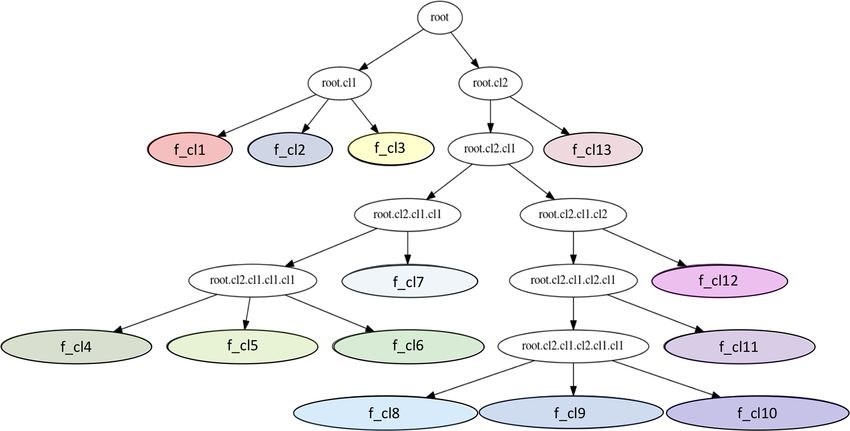
M. Lukach et al.: Hydrometeor classification of QVPs using a top-down hierarchical clustering                                                  1083

Figure 4. The active clusters at the end of the first (a, b) and second (c, d) cycle of the outer loop of the hierarchical clustering algorithm.
Panels (a) and (c) are plotted in the hierarchical (tree) structure, and panels (b) and (d) are plotted in height vs. time format of the observations
on 17 May 2017.

tailization”, the optimal clustering for the provided input data             sults to the literature. Labelling the obtained clusters can be
has been reached. For the QVP dataset described in Sect. 3,                  performed for the different levels of granularity depending
a final set of 13 active clusters is reached (see Figs. 5 and 6).            on the user’s needs and interests. Note the purpose of the
The relations between these final clusters (f_cl1,. . ., f_cl13)             labelling shown here is to demonstrate the ability and valid-
and the three parent clusters from the first inner loop run                  ity of the technique rather than performing a rigorous study
(Fig. 4a) are shown in Fig. 5.                                               of the underlying microphysics observed. The latter will be
                                                                             reserved for follow-up studies utilizing this technique in a
                                                                             focused manner.
5   Labelling
                                                                             5.1    Level-by-level cluster check
Once the optimal number of clusters is determined and the
hierarchical clustering structure is built, the clusters can be              From the visual verification of the first-level parent clusters
characterized by their centroids and labelled with appropriate               in Fig. 4a and b, we can deduce that there are two child
hydrometeor classes using the available verification data. The               clusters representing the upper or elevated (ice-dominated
clusters for which direct verification data are not available                root.cl2) and the lower (water-dominated root.cl1) parts.
may still be labelled with an appropriate hydrometeor class                  The second-level clusters from the second loop (Fig. 4c
based on the scattering characteristics described by the orig-               and d) show a well-identified “bright band” (root.cl2.cl2),
inal polarimetric radar variables and considering their posi-                belonging to the melting layer (ML), and a main solid-
tion in the hierarchical tree and the height vs. time QVP rep-               phase cluster (root.cl2.cl1), both belonging to the cluster
resentation. As QVP polarimetric characteristics differ from                 representing the ice-phase-dominated part (root.cl2) of the
polarimetric characteristics of hydrometeors observed by PPI                 QVPs (Fig. 4b). The three child clusters of the parent
and RHI scans, care must be taken when comparing these re-                   root.cl1 cluster (Fig. 4c and d) are the two rain-type clus-

https://doi.org/10.5194/amt-14-1075-2021                                                         Atmos. Meas. Tech., 14, 1075–1098, 2021
1084 M. Lukach et al.: Hydrometeor classification of QVPs using a top-down hierarchical clustering
Figure 5. Final hierarchical structure of the optimal clustering found for the QVP input data described in Table 1. The final set of optimal
clusters consists of coloured clusters f_cl1, f_cl2,. . ., f_cl13.
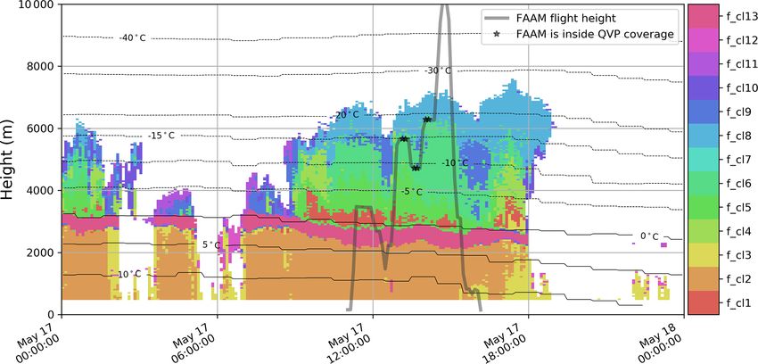
Figure 6. The height vs. time format of the final optimal set of active clusters found by the top-down hierarchical clustering for the QVP
input data described in Table 1. (The hierarchical structure behind the optimal clustering is found in Fig. 4.) Example of clusters in the height
vs. time format of the 17 May 2017 QVPs presented in Fig. 2.
ters (root.cl1.cl2 and root.cl1.cl3) below the “bright band” 5.2 Characteristics of the clusters
and cluster root.cl1.cl1 with most points located above the
“bright band”. In further loops, the main ice-phase cluster The 13 final clusters can be characterized by their centroids
(root.cl2.cl1) is split into nine child clusters (Fig. 5), and ex- (Fig. 7) or their relevant statistics (Fig. 8, Table A1). The cen-
amples of their positioning in the height vs. time format of troid characteristics in Fig. 7 are plotted as spider plots where
QVPs can be observed in Fig. 6 or Fig. B1. each of the five variables is represented by an azimuthal axis.
The filled pentagons in each sub-plot represent the cluster’s
centroid in the five-variable space based on all the data avail-
able in this study. Each vertex of the pentagon shows the cen-
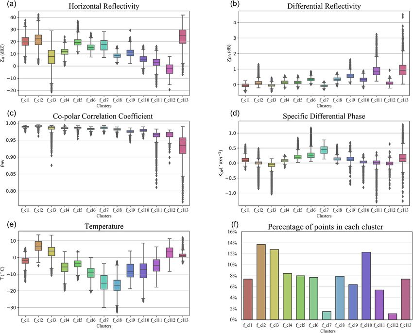
Atmos. Meas. Tech., 14, 1075–1098, 2021 https://doi.org/10.5194/amt-14-1075-2021M. Lukach et al.: Hydrometeor classification of QVPs using a top-down hierarchical clustering 1085 troid’s value in one of the five variables. The non-solid lines ter has no variation in temperature (T ), with all centroids at in the sub-plots of Fig. 7 represent the centroids of the same 0 ◦ C. As such, f_cl13 corresponds to the area in the data cluster but based solely on the data from one of the eight referred to as a “bright band”. According to the box and cases (Table 1). whiskers plots in Fig. 8, cluster f_cl13 has the highest mean Figure 7 confirms a distinction made at the first and the ZH (24 dBZ) and mean ZDR (0.99 dB) as well as the lowest second cycles of the outer loop (Fig. 4) between three types mean ρHV (0.93) compared with the other optimal clusters, of clusters: liquid-phase clusters (f_cl1, f_cl2 and f_cl3), and it is mostly located near 0 ◦ C. These characteristics im- with lower KDP and warmer T values; ice-phase clusters mediately indicate that f_cl13 can be labelled as belonging to (f_cl4, f_cl5, f_cl6, f_cl7, f_cl8, f_cl9, f_cl10, f_cl11, and the “bright band” cluster with mixed-phase (MP) particles. f_cl12), all with more pronounced ρHV values; and a very The MP cluster (f_cl13 in Fig. 6) is observed to have some different looking f_cl13, with warmer T and rather low ρHV sagging areas: between 10:00 UTC and 12:20 UTC, around values. 16:00 UTC and near 18:00 UTC. Note that f_cl1 is observed The largest differences between the centroids selected above the MP cluster f_cl13 exactly at these time intervals from the total dataset and the centroids corresponding to the (Fig. 6). This sagging “bright band” signature is often ob- eight considered cases occur in the temperature (T ) values, served where aggregation and riming processes are occur- especially for the clusters f_cl2, f_cl3, f_cl7, f_8, f_cl10 and ring directly above the melting layer (Kumjian et al., 2016; f_cl12. These variations can be explained by the origin of the Ryzhkov and Zrnic, 2019). This suggests that f_cl1 can be temperature data, which are estimates from the NWP model associated with the processes of aggregation or riming and and do not always correctly represent the real situation. labelled accordingly. The next variable with a rather large variation in several Looking at the percentage of points belonging to each clusters is KDP . In part, this variation may be due to the fact cluster in the optimal clustering set (Fig. 8f), we see that that this variable has an extremely skewed distribution. Clus- clusters f_cl7 and f_cl12 have less than 2 % of points and ters f_cl1, f_cl7, f_cl11, f_cl12 and f_cl13 have the high- most probably represent some sporadic and/or special con- est variation in KDP values between the centroids calculated ditions. These clusters have also been separated early from for different cases (Fig. 7). As KDP can be influenced by the the other “low ice” (f_cl4, f_cl5, f_cl6) and “elevated ice” amount of ice or water particles in the atmosphere, it might (f_cl8, f_cl9, f_cl10, f_cl11) clusters and are located near the be that the clusters have variations in the number of particles. top of the hierarchical tree (Fig. 5). Both clusters f_cl7 and This hypothesis can only be verified with FAAM BAe 146 f_cl12 have smaller absolute mean ZDR values (−0.062 and observations of the same cluster on different dates. Unfortu- 0.097 dB respectively) than the other “ice” clusters (Fig. 8b). nately, such verification is not possible for all clusters, and f_cl7 is also characterized by the highest mean KDP value more in situ observations are required. (0.44◦ km−1 ) among all of the clusters (Fig. 8d). The com- From the variations of centroid values in the five input bination of rather high ZH (17 dBZ) and high KDP at tem- variables in Fig. 7, we can also see that the main liquid-phase peratures around −15 ◦ C indicates a cluster with high parti- cluster (f_cl2) has rather different characteristics in different cle number concentration of small ice crystals mixed with a cases. Case to case it shows large variations in ZH , KDP , ρHV , small amount of bigger aggregates. This cluster is potentially T and the highest mean temperature value (6.8 ◦ C) among all a manifestation of the rapid growth of ice via vapour deposi- other clusters. As observed in the histogram of percentages tion and the onset of aggregation in the dendritic growth layer of the cluster points in Fig. 8f, f_cl2 is rather big (13.7 % (DGL) discussed in detail in Griffin et al. (2018). These char- of the total number of points) but does not have the highest acteristics were also recognized as a signature of dendritic percentages of points in all eight analysed cases, only in the crystals in Bechini et al. (2013). f_cl12 has the lowest mean 17 May 2017 case (9.3 % compared with ≤ 1.5 % in other ZH value (−3 dBZ) of all optimal clusters. Combining the cases) (Fig. 7, histogram in the lower right corner.). Combin- low mean ZH with low mean ZDR (0.097 dB) and a tempera- ing all of these aspects, we deduce that f_cl2 includes rain of ture of about 3 ◦ C, we can assume that f_cl12 can be labelled varying intensities and different drop sizes. as small droplets (i.e. drizzle). The other rain cluster f_cl3 has less variability in cen- f_cl11 belongs to the “elevated ice” clusters and in most troid values and has ∼ 20 dBZ smaller ZH values than f_cl2, cases (see Appendix B, Fig. B1) appears as a column in the which is probably due to the smaller drop sizes in this cluster. height vs. time representation (around 07:00 UTC in Fig. 6 f_cl3 has the smallest mean ZH (7.18 dBZ) and mean KDP or in panels (a) 07:00–08:00 UTC, (c) 05:00 and 07:30 UTC, values (−0.097◦ km−1 ) of all “water” clusters (f_cl1, f_cl2 (g) 12:00 UTC and (h) 12:00–12:30 UTC in Fig. B1) filling and f_cl3). This cluster is often observed at the beginning all of the altitudes from the top of the cloud to the ML. This and at the end of the storm in the height vs. time format rep- cluster has a low mean ZH value (3 dBZ), one of the highest resentation of the optimal clusters (Fig. B1) and is labelled mean ZDR values (0.92 dB) and a close to zero mean KDP as “light rain”. value (−0.009◦ km−1 ). f_cl11 can be labelled as the pristine Almost all centroids in Fig. 7 have no or very limited vari- ice crystals class, as they typically have high aspect ratios ation in the ρHV or ZDR values except for f_cl13. This clus- https://doi.org/10.5194/amt-14-1075-2021 Atmos. Meas. Tech., 14, 1075–1098, 2021
1086                        M. Lukach et al.: Hydrometeor classification of QVPs using a top-down hierarchical clustering

Figure 7. Characteristics of the optimal clustering centroids in four polarimetric variables and temperature. The scales of the variables are
as follows: from −20 to 40 dBZ for ZH , from −1.5 to 2.0 dB for ZDR , from 0.9 to 1.0 for ρHV , from −0.3 to 0.6◦ km−1 for KDP and from
−20 to 10 ◦ C for temperature (T ).

Atmos. Meas. Tech., 14, 1075–1098, 2021                                                    https://doi.org/10.5194/amt-14-1075-2021
M. Lukach et al.: Hydrometeor classification of QVPs using a top-down hierarchical clustering                                       1087

Figure 8. Characteristics of the optimal clustering centroids in four polarimetric variables (a – ZH , b – ZDR , c – ρHV and d – KDP ) and
temperature (e). The percentage of points in each cluster is shown in panel (f).

( 1) and tend to fall preferentially with their major axis            the time it is located near f_cl8 at the beginning or at the end
aligned horizontally (Keat and Westbrook, 2017).                       of the observed event (Fig. B1).
   Clusters f_cl8, f_cl9 and f_cl10 belong to the “elevated               The main “low ice” clusters are f_cl4, f_cl5 and f_cl6.
ice” branch of the hierarchical tree (Fig. 5). Among these             Clusters f_cl5 and f_cl6 are often observed together with
clusters, f_cl9 has the most different characteristics com-            f_cl6 located above f_cl5. f_cl4 has several appearances
pared to the f_cl8 and f_cl10 clusters. f_cl9 has higher mean          in the height vs. time formats of events (see Appendix B,
ZH (11 dBZ) and ZDR (0.59 dB) in combination with a lower              Fig. B1, e.g. 09:00 UTC in panel a, 11:00 UTC in panel b,
ρHV (0.97).                                                            09:00 and 17:00-18:00 UTC in panel e), mostly above f_cl1,
   f_cl8 and f_cl10 have rather similar characteristics to             reaching higher altitudes in the data.
each other (Fig. 7, Table A1). The small difference between               Measurement errors may influence the clustering results.
these two clusters is in a higher mean ZH (8.6 dBZ) and                As was shown by Bringi et al. (1990), noise in the obser-
KDP (0.14◦ km−1 ) for f_cl8 compared with 5.8 dBZ and                  vations has a strong impact on k-mean HCA (hierarchical
0.028◦ km−1 for f_cl10. Both clusters are the main “ele-               clustering algorithm) results. Unfortunately, it is impossi-
vated ice” clusters. f_cl10 has a warmer mean temperature              ble to run the same type of analysis conducted by Bringi
(−8.2 ◦ C compared with −16.7 ◦ C for f_cl8), and most of              et al. (1990) for an unsupervised hierarchical clustering al-
                                                                       gorithm, as the added noise might deliver a modified hier-

https://doi.org/10.5194/amt-14-1075-2021                                                  Atmos. Meas. Tech., 14, 1075–1098, 2021
1088 M. Lukach et al.: Hydrometeor classification of QVPs using a top-down hierarchical clustering
archical structure with another optimal number of clusters, which appear round (Figs. 9a–c, 10a–c). This strongly rein-
and direct comparison to the original set of final clusters forces the idea of large amounts of liquid water being present
would be impossible. Here, this issue of noise is partially in the cloud, which supports the labelling of f_cl1–f_cl3 as
addressed through our use of QVPs. In particular, azimuthal being influenced by liquid water hydrometeors. When look-
averaging of a QVP reduces the noisiness of the differential ing at CIP100 in situ observations in detail, and to some ex-
phase within the melting layer (Trömel et al., 2013, 2014) tent CIP15 observations at sizes > 200 µm, we can see some
and was recommended in Kumjian et al. (2013) to quantify significant difference between clusters f_cl1–f_cl3, which
rather small enhancements of ZDR and KDP . we will now discuss.
The mean negative values of ZDR and KDP in some clus- f_cl1, observed above the “bright band”, was previously
ters (f_cl1, f_cl3 and f_cl7) might point at potential biases assigned to be the result of aggregation and riming. In this re-
due to the miscalibration of ZDR , differential attenuation or gion, the CIP100 (Fig. 9, lower part of panel a) shows particle
backscatter differential phase in the melting layer. Biases in imagery and particle size distributions segregated by shape
the data such as miscalibration will not impact the cluster- that show the presence of large ice particles (Fig. 10a), again
ing process but will impact the labelling, as it is based on confirming the previous cluster labelling. The CIP100 data
cluster characteristics. A miscalibration of ZDR can also be show the presence of irregularly shaped particles, ranging in
excluded, as we routinely perform calibration of this vari- size from ∼ 1 to 4 mm, with concentrations in each bin of the
able. ZH and ZDR are corrected for the attenuation in the order of 1 m−3 . This suggests that a mode of snow particles
data preprocessing. Biases caused by backscatter differential is present at the same time as the previously mentioned liq-
phase in the melting layer (Trömel et al., 2014) have not been uid droplet mode. Many small water droplets in the CIP15
removed and are evident in the cluster characteristics. The observations (Figs. 9a and 10a, CIP15) could indicate either
influence of the backscatter differential phase needs further the presence of warm cloud processes or small ice crystals
investigation. As discussed, not all clusters can be labelled melting first around the ML. The second interpretation is sup-
with absolute confidence solely based on the cluster’s char- ported by the imagery from the CIP100 which suggests melt-
acteristics, and in situ observations can help to verify these ing has not started to occur on the larger particles. In this
initial suppositions. case, the larger aggregate snowflakes fall to lower altitudes
before they start to melt and form the clear “bright band” in
5.3 Clusters vs. in situ observations the QVPs.
f_cl2 was characterized by the strong variation in ZH ,
5.3.1 In situ data KDP , ρHV and T of the cluster’s centroids in different cases.
Both CIP15 and CIP100 have small round-shaped particles
For the verification of the preliminary labelling made in in the corresponding images (Fig. 9b). The mean concentra-
Sect. 5.2, data from the CIP15 and CIP100 on board the tions per particle size distributions (Fig. 10b) show the preva-
FAAM BAe 146 are utilized. FAAM BAe 146 aircraft flights lence of particles recognized by shape as water droplets. The
were performed on 4 out of 8 d (Table 1) of radar observa- droplets of < 2 mm size have the occurrences of the order of
tions: 17 May 2017, 24 January 2018, 13 February 2018 and 10 to 90 000 m−3 , with higher orders corresponding to par-
14 February 2018. The flight altitudes and the time stamps ticle sizes < 200 µm. Summing up previous analysis and in
when the aircraft was inside the QVP domain can be ob- situ observations, we can assign f_cl2 to a “liquid” cluster,
served in the height vs. time representations of the optimal which includes rain of varying intensities and different drop
clusters in Fig. B1. sizes.
Out of the four available flights, there are 23 periods of 20 s f_cl3 also has predominantly small round-shaped particles
intervals which result in a total of 460 s of flight time when (mean size µ = 128 µm) in the CIP15 panels (Figs. 9 and 10,
the aircraft was inside the QVP domain and a cluster can upper part of panel c). The CIP100 data (Fig. 9, lower part of
be assigned to the corresponding height. Of these 23 periods panel c) were not processed due to technical issues with the
there are observations corresponding to nine unique clusters probe, so water or ice concentrations based on this data are
(f_cl1, f_cl2, f_cl3, f_cl4, f_cl5, f_cl6, f_cl8, f_cl10, f_cl12). unfortunately not available. The high concentrations (1000–
This samples 70 % of the final clusters. From these time se- 5000 m−3 ) of small size (< 200 µm) particles are assigned
ries, we present examples of CIP15 and CIP100 images for to water (Fig. 10c). Concentrations of the larger particles (>
each cluster (Fig. 9) and mean particle size distributions of 200 and < 800 µm) are very low (< 100 m−3 ). Considering
the data observed during the 20 s interval (Fig. 10). these observations, the cluster’s characteristics, and the fact
that the cluster appears mostly at the beginning or at the end
5.3.2 Liquid-phase clusters of the events (Fig. B1), we can assume that the cluster either
represents very light rain or drizzle or indicates a partially
The liquid-phase clusters f_cl1, f_cl2 and f_cl3 correspond filled QVP domain in the original data.
to in situ data that contain relatively high concentrations
(> 1000 m−3 ) of small particles (mostly < 200 µm in size)
Atmos. Meas. Tech., 14, 1075–1098, 2021 https://doi.org/10.5194/amt-14-1075-2021You can also read