Prediction of Satellite-Based Column CO2 Concentration by Combining Emission Inventory and LULC Information - TUM
←
→
Page content transcription
If your browser does not render page correctly, please read the page content below
This article has been accepted for inclusion in a future issue of this journal. Content is final as presented, with the exception of pagination.
IEEE TRANSACTIONS ON GEOSCIENCE AND REMOTE SENSING 1
Prediction of Satellite-Based Column CO2
Concentration by Combining Emission
Inventory and LULC Information
Shrutilipi Bhattacharjee , Member, IEEE, and Jia Chen , Member, IEEE
Abstract— In this article, we generate a regional mapping of
space-borne carbon dioxide (CO2 ) concentration through a data
fusion approach, including emission estimates and Land Use
and Land Cover (LULC) information. NASA’s Orbiting Carbon
Observatory-2 (OCO-2) satellite measures the column-averaged
CO2 dry air mole fraction (XCO2 ) as contiguous parallelogram
footprints. A major hindrance of this data set, specifically with
its Level-2 observations, is missing footprints at certain time
instants and the sparse sampling density in time. This article
aims to generate Level-3 XCO2 maps on a regional scale for
different locations worldwide through spatial interpolation of
the OCO-2 retrievals. To deal with the sparse OCO-2 sam-
pling, the cokriging-based spatial interpolation methods are
suitable, which models auxiliary densely-sampled variables to
predict the primary variable. In this article, a cokriging-based
approach is applied using auxiliary emission data sets and
the principles of the semantic kriging (SemK) method. Two
global high-resolution emission data sets, the Open-source Data
Inventory for Anthropogenic CO2 (ODIAC) and the Emissions
Database for Global Atmospheric Research (EDGAR), are used
here. The ontology-based semantic analysis of the SemK method
quantifies the interrelationships of LULC classes for analyzing
the local XCO2 pattern. Validations have been carried out in
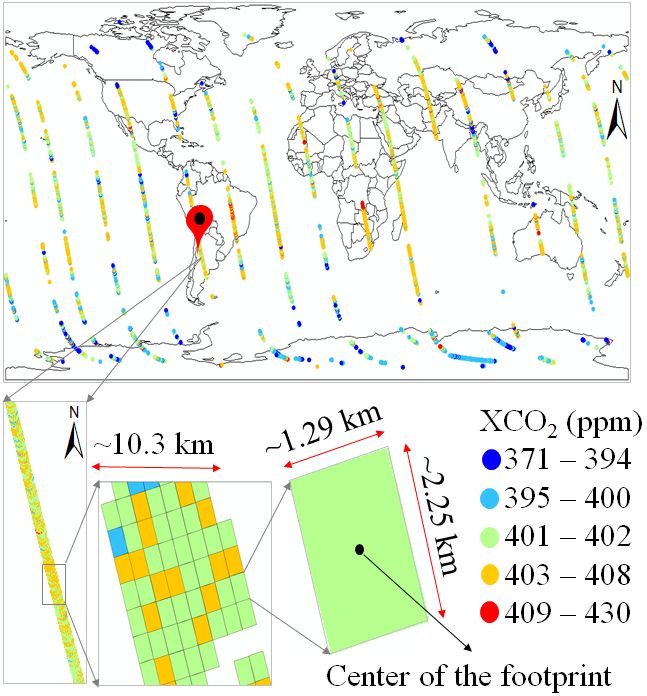
different regions worldwide, where the OCO-2 and the Total Fig. 1. XCO2 measurements by OCO-2 on October 14, 2017.
Carbon Column Observing Network (TCCON) measurements
coexist. It is observed that the modeling of auxiliary emission Exploratory Satellite for Atmospheric CO2 (TanSat) [3],
data sets enhances the prediction accuracy of XCO2 . This article
Japanese GHGs Observing SATellite (GOSAT) [4], and Envi-
is one of the initial attempts to generate Level-3 XCO2 mapping of
OCO-2 through a data fusion approach using emission data sets. ronmental Satellite (ENVISAT) [5]. The OCO-2 measures
the column-averaged CO2 dry air mole fractions (XCO2 ) in
Index Terms— Emissions Database for Global Atmospheric
Research (EDGAR), interpolation, land use and land cover
the atmosphere as contiguous parallelogram footprints, each
(LULC), Orbiting Carbon Observatory-2 (OCO-2), Open-source having area up to about 3 km2 . The XCO2 measurements are
Data Inventory for Anthropogenic CO2 (ODIAC), semantic obtained using a number of retrieval algorithms, for example,
kriging (SemK), column-averaged CO2 dry air mole fractions NASA Atmospheric CO2 Observations from Space (ACOS)
(XCO2 ). algorithm [6]. However, these are Level-2 retrievals and irreg-
I. I NTRODUCTION ular in space as well as in time. Fig. 1 shows the OCO-2
Lite Version 9r XCO2 measurements on October 14, 2017.
A TMOSPHERIC carbon dioxide (CO2 ) is a greenhouse
gas (GHG) that affects climate change most significantly.
A number of satellites were launched in the last few years
A portion of a measurement swath near Córdoba, Argentina,
is magnified where the parallelogram footprints are visible
that were dedicated to GHG observations. Examples include, and the corresponding swath width (approximaely10.3 km [7])
NASA’s Orbiting Carbon Observatory-2 (OCO-2) [1], [2], is shown. One footprint is further magnified to show its
maximum dimension. The center of the parallelogram is the
Manuscript received December 14, 2018; revised June 14, 2019, representative center point of the sounding footprint. The
December 3, 2019, and January 20, 2020; accepted January 30, 2020. This XCO2 values of these one-day retrievals are categorized into
work was supported in part by the Technical University of Munich - Institute
for Advanced Study through the German Excellence Initiative and the five classes (shown in different colors), and the measurement
European Union Seventh Framework Program under Grant n◦ 291763 and unit is parts per million (ppm, 10−6 ). It is evident from the
in part by the German Research Foundation (DFG) under Grant 419317138. figure that, on a single day, a huge portion of the Earth’s
(Corresponding authors: Shrutilipi Bhattacharjee; Jia Chen.)
The authors are with the Department of Electrical and Computer Engi- surface remains unmeasured, and this problem eventually
neering, Technical University of Munich, 80333 Munich, Germany (e-mail: propagates in its time-series measurements as well.
shrutilipi.bhattacharjee@tum.de; jia.chen@tum.de). This incomplete sampling of atmospheric CO2 prevents us
Color versions of one or more of the figures in this article are available
online at http://ieeexplore.ieee.org. from understanding the global carbon cycle, the mechanisms
Digital Object Identifier 10.1109/TGRS.2020.2985047 to control its spatial and temporal variability, the distributions
0196-2892 © 2020 IEEE. Personal use is permitted, but republication/redistribution requires IEEE permission.
See https://www.ieee.org/publications/rights/index.html for more information.
Authorized licensed use limited to: Technische Universitaet Muenchen. Downloaded on May 19,2020 at 17:14:05 UTC from IEEE Xplore. Restrictions apply.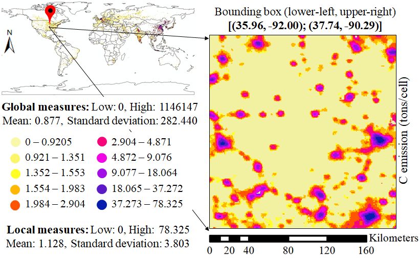
This article has been accepted for inclusion in a future issue of this journal. Content is final as presented, with the exception of pagination.

2                                                                                                                 IEEE TRANSACTIONS ON GEOSCIENCE AND REMOTE SENSING

of carbon emission and uptake, and so on. Apart from the                                         methods, the geostatistical interpolation methods or kriging
satellite remote sensing of CO2 , several high-resolution                                        are reported to be more accurate. Among the geostatistical
globally gridded emission inventories are available, which                                       interpolation methods, the variants of kriging, for example,
represents the anthropogenic emissions from different                                            simple kriging (SK) [13], ordinary kriging (OK) [14], universal
activities. For example, the Open-source Data Inventory for                                      kriging (UK) [15], spatial block kriging (BK) [16], fixed rank
Anthropogenic CO2 (ODIAC) is one such popular emission                                           kriging (FRK) [17], [18], ordinary cokriging (OCK) [19], and
data product. It is based on the latest country FFCO2 estimates                                  spatiotemporal kriging (STK) [20], are popular spatial and spa-
(2000–2015) made by the Carbon Dioxide Information                                               tiotemporal methods to generate a Level-3 mapping from the
Analysis Center (CDIAC) at the Oak Ridge National Lab                                            satellite-based Level-2 retrievals and other related applications.
(ORNL), USA, by fuel type (solid, liquid, gas, cement                                            Among other nongeostatistical interpolation methods, inverse
manufacturing, gas flaring, domestic/international shipping,                                     distance weighting (IDW), nearest neighbor (NN), thin-plate
aviation, and marine bunkers) [8]. Currently, it provides                                        spline (TPS), and trend surface analysis (TSA) are a few
monthly emission data from 2000 to 2017. According to Oda                                        popular methods [21]. Many studies have reported that the
et al. [8], this data can be considered for the modeling of                                      terrestrial land use and land cover (LULC) change have a
remotely sensed XCO2 data from the OCO-2 satellite for                                           profound impact on the increase of atmospheric CO2 . For
understanding the carbon cycle science. Similarly, another                                       example, Houghton [22] and Houghton and Goodale [23]
comprehensive database of anthropogenic GHG emissions                                            have stated that the changes in LULC, such as cropland
is the Emissions Database for Global Atmospheric Research                                        expansion, resulted in the release of 156 Pg of carbon to
(EDGAR) [9]. It provides time-series fossil CO2 emission                                         the atmosphere during the period between 1850 and 1990.
estimates from 1970 to 2012, including anthropogenic                                             They reported this amount to be half of the carbon released
emissions from fossil fuel combustion and production, as well                                    from the combustion of fossil fuels over the same period.
as from industrial processes (cement, steel, liming, urea, and                                   Hwang and Um [24] have presented an interesting study
ammonia production, or consumption). These emissions are                                         to find the causal relationship between LULC and carbon
calculated with a bottom–up approach using international                                         emissions using OCO-2’s XCO2 data. They have reported
statistics for the activity data (such as fuel consumption                                       that the LULC classes representing the development activ-
or crops) and Intergovernmental Panel on Climate Change                                          ities generally exhibit higher mean XCO2 compared with
(IPCC) (2006) values for the emission factors. The uncertainty                                   the nonanthropogenic LULC types. Therefore, the terrestrial
for the global annual anthropogenic CO2 emission estimate                                        LULC distribution is significant information to be modeled
ranges from −9% to +9% [10]. However, the uncertainties of                                       for the mapping of XCO2 alongside the emission estimates.
the GHG inventory vary from nation to nation and are much                                        For this article, the underlying terrestrial distribution of LULC
higher. For example, the estimated uncertainties (2σ ) reported                                  and their influences on the local XCO2 pattern have to be
for CO2eq in China, India, and Brazil are 11.3%, 17.2%,                                          quantified so that it can be used in any cokriging framework.
and 28.3%, respectively, in 2012 [10]. In the subnational                                        Here, we have used the semantic modeling component of
scale, the uncertainty is even higher [11]. Considering these                                    the semantic-kriging-(SemK)-based interpolation method [25].
emissions to be the major contributing factors to the expansion                                  This semantic modeling adopts an ontology-based approach to
of CO2 in the atmosphere, this article aims to predict the                                       quantify the terrestrial LULC classes for analyzing different
missing XCO2 concentrations of OCO-2 by contemplating                                            environmental variables [26], [27]. This quantified LULC,
the emission estimates of ODIAC or EDGAR as the auxiliary                                        along with the auxiliary emission data sets, is inserted into a
information into the prediction process. The 2017 ODIAC                                          traditional cokriging [19] process. This approach is referred to
estimates (monthwise) and 2012 EDGAR estimates are used in                                       as cokriging with semantic analysis of LULC (SemCK) [28].
this article. There is a temporal misalignment of the EDGAR                                      The broader objectives are as follows.
emission data set with the 2017 OCO-2 measurements                                                  1) Spatial interpolation of sparse Level-2 XCO2 measure-
considered in the empirical study. According to [12], global                                            ments of OCO-2 to create a Level-3 mapping at a
GHG emissions are dominated by the fossil CO2 share and                                                 particular time instance in a local region.
steadily increased in the period between 1970 and 2012. Then,                                       2) Semantically quantifying the auxiliary variable LULC
the global CO2 emissions show a slowdown trend and were                                                 alongside the emission estimates from ODIAC or
stalled for the third year in a row with no further increment                                           EDGAR for the primary variable (XCO2 from OCO-2).
of the total CO2 in 2016. Therefore, the EDGAR emission                                             3) Validations by comparing the traditional baseline alter-
estimate from 2012 can be used as a valid data set for this                                             native with respect to its extensions with LULC and
article. Since, here we try to differentiate between the high-                                          emission data.
and low-emission zones through the emission estimates of a                                          4) Comparison of the prediction results with the external
local region, the temporal stability assumption of this auxiliary                                       Total Carbon Column Observing Network (TCCON)
data should not affect the performance of this approach. The                                            data.
empirical results also justify this assumption in Section V.                                        The rest of this article is organized as follows. Section II
   To address the drawback of the incomplete OCO-2 mea-                                          presents the recent works on creating a Level-3 XCO2
surements stated earlier, spatial prediction, more specifically                                  map from the satellite measurements. Section III describes
spatial interpolation, is one of the obvious choices reported in                                 the SemCK approach focusing on the LULC quantification
the literature. In contrast to the deterministic spatial prediction                              process of the SemK method. In Section IV, different data sets

    Authorized licensed use limited to: Technische Universitaet Muenchen. Downloaded on May 19,2020 at 17:14:05 UTC from IEEE Xplore. Restrictions apply.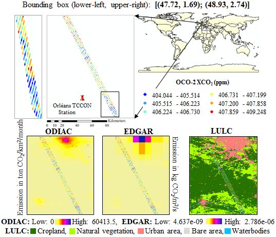
This article has been accepted for inclusion in a future issue of this journal. Content is final as presented, with the exception of pagination.

BHATTACHARJEE AND CHEN: PREDICTION OF SATELLITE-BASED COLUMN CO2 CONCENTRATION                                                                                           3

considered in this article and the specifications of the empirical                              fusion technique to generate a global distribution of XCO2 by
study have been presented. Section V presents the interpolation                                 fusing GOSAT and SCIAMACHY CO2 measurements. The
results of XCO2 and other analytical results. Discussions to                                    OK-based interpolation method applied to this data fusion
understand the XCO2 mapping application and the SemCK                                           approach has increased the spatial coverage up to approxi-
approach are presented in Section VI. Finally, the conclu-                                      mately 20% compared with a single data set. Wang et al. [36]
sions are presented in Section VII, including some future                                       have also proposed a method for fusing SCIAMACHY and
prospects.                                                                                      GOSAT XCO2 measurements. This amalgamation approach
                                                                                                has increased the global spatial coverage of XCO2 by 41.3%
                                                                                                on a daily and 47.7% on a monthly temporal scale, relative to
                       II. R ELATED W ORKS
                                                                                                the measurements of GOSAT. Compared with SCIAMACHY,
   The literature has been reported on different appli-                                         this article reports even higher spatial coverage. Similarly,
cations of the XCO2 data from the OCO-2 satellite.                                              Watanabe et al. [37] and Liu et al. [38] have applied kriging
Zammit-Mangion et al. [17] have indicated that the gap-filled                                   interpolation methods to generate a Level-3 spatial distribution
Level-3 XCO2 product can be used for validating the                                             of GOSAT XCO2 . Nguyen et al. [39] have proposed a method
OCO-2 retrievals against ground-based measurements or                                           for fusing the vertical profiles of XCO2 from OCO-2 and
atmospheric transport model output. A few attempts have                                         GOSAT. The modified spatial random effects model, applied
been made to generate a comprehensive Level-3 mapping                                           on the CO2 profiles, has reduced the mean squared error of
of XCO2 from the partially sampled Level-2 retrievals                                           data fusion in comparison with the TCCON measurements.
of the OCO-2 satellite. Article [17] is one such recent                                            From the methodology perspective, the abovementioned
work that is reported on generating full coverage satel-                                        literature on the XCO2 mapping has used different predic-
lite Level-3 mapping from the Level-2 product of OCO-2.                                         tion algorithms. The OK-based interpolation approach is a
Zammit-Mangion et al. [17] have developed a spatiotemporal                                      basic, univariate, minimum variance, linear, unbiased mapping
statistical modeling framework of FRK to obtain the global                                      method. The SK assumes the mean of the random field to
predictions of XCO2 with Version 7r and Version 8r data                                         be known and constant over the study region (SR). The UK
of OCO-2. They have validated the prediction framework                                          approach is a variant of OK, which analyzes the local trend
with TCCON data [29] and found that the Version 8r per-                                         within a predefined search window around the prediction
forms better than the Version 7r. Chevallier et al. [30] have                                   point as a continuous and smoothly varying function of the
attempted to generate a global continuous map of XCO2 at                                        sampled locations [13]. The BK method can extend any basic
daily and monthly temporal resolutions. They have considered                                    kriging method (such as OK and UK) and uses the average
a Bayesian Kalman filter (KF) developed on a model of                                           expected value over a segment/surface/volume around the
persistence and compared the KF daily-mean XCO2 maps                                            prediction point. The point-to-point covariance of the basic
with TCCON data. Hammerling et al. [31] have adopted a                                          kriging is replaced by the point-to-block covariance [13]. The
statistical mapping approach for creating a full coverage of                                    FRK makes the kriging interpolation process efficient to deal
the atmospheric CO2 that is synthetically generated from                                        with a very large sample size. The reduced complexity in
the PCTM/GEOS-4/CASA-GFED model. They have reported                                             the prediction and error computation process in the FRK is
that the overall uncertainty in terms of root-mean-square                                       achieved by the choice of covariance function to offer an
prediction error (RMSPE) ranges from 0.20 to 0.63 ppm.                                          efficient way to compute the kriging equations [17], [18]. The
The prediction accuracy varies with the temporal averaging                                      space–time kriging [20], [40] method is a variant of the basic
window (1-day, 4-day, 16-day, and so on) and season (such                                       spatial interpolation process to include the time component.
as January, April, July, and September). The highest and                                        It decomposes the random function into a deterministic trend
lowest RMPSEs are observed with the combination of one-day                                      component (representing the spatial trend and the temporal
averaging window in July and 16-day window in September,                                        trend) and a residual component (representing a stationary
respectively.                                                                                   space–time error process). Similarly, the cokriging extension
   From the application perspective, similar attempts have been                                 of the basic kriging modifies the baseline method for multi-
reported to generate a Level-3 XCO2 mapping with other                                          variate analysis [41] to intake multiple variables as input when
satellite data as well. Zeng et al. [32] have implemented a                                     the prediction variable is sparsely sampled [13], [19].
space–time kriging with a moving flexible kriging neigh-                                           The assessment of satellite-derived XCO2 measurements
borhood for the ACOS-GOSAT XCO2 data set. They have                                             and the CO2 emission estimates for each other has been
validated the prediction results in three ways: through a                                       found in different applications, for example, to determine the
cross-validation approach, in comparison with TCCON data,                                       impact of regional fossil fuel emissions on global XCO2 fields
and with the model-based simulated data from both Carbon-                                       [42], estimate the fire CO2 emission by using XCO2 [43],
Tracker CT2013 [33] and GEOS-Chem [34]. Tadić et al. [16]                                      determine CO2 emissions from megacities by using XCO2
have proposed a flexible moving window BK method to                                             through inverse modeling approach [44] or from the individual
generate a Level-3 continuous map of satellite data and                                         middle to large-sized coal power plants through plume model
applied this method for two data sets: the XCO2 from the                                        simulations [45], and observe the anthropogenic CO2 emis-
GOSAT satellite and the solar-induced fluorescence (SIF)                                        sion by deriving CO2 anomalies through deseasonalizing and
from the Global Ozone Monitoring Experiment-2 (GOME-2)                                          detrending XCO2 measurements [46]. This article is one of
instrument [35]. Jing et al. [14] have proposed a new data                                      the initial attempts for modeling the emission inventories as

   Authorized licensed use limited to: Technische Universitaet Muenchen. Downloaded on May 19,2020 at 17:14:05 UTC from IEEE Xplore. Restrictions apply.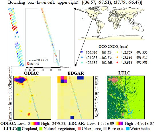
This article has been accepted for inclusion in a future issue of this journal. Content is final as presented, with the exception of pagination.

4                                                                                                                 IEEE TRANSACTIONS ON GEOSCIENCE AND REMOTE SENSING

auxiliary variables to generate a mapping surface of
space-borne XCO2 measurements of OCO-2.

                         III. M ETHODOLOGY
   From the literature, it is evident that the geostatistical
interpolators, mainly different variants of kriging, are the most
widely used techniques for creating a complete mapping from
sparsely sampled data. However, variety exists depending on
several factors, such as accuracy-complexity tradeoff, smooth-
ing factor of the predictor, available observed/sampled loca-
tions, and type of auxiliary information. Here, we have used
a cokriging approach that intakes quantified LULC and the
emission estimates as the covariates. Our previously proposed
SemK-based interpolation method [25], [47] has two compo-
nents: the quantification of LULC classes for the environmen-
tal variables that are inherently influenced by or dependent on                                  Fig. 2.     A LULC ontology.
the terrestrial LULC dynamics through semantic modeling,
and the updating of the traditional Euclidean-distance-based
dependences with this semantic modeling. The kriging is often                                    The OK is similar to SK but replaces μ in  N(1) with a local
regarded as a “smooth” interpolator that is detrimental to the                                   mean μ(x 0 ), which leads to the condition i=1  wi = 1.
prediction outcome. The SemK models the LULC to deal
with the underlying terrestrial distribution. It aims to reduce                                  B. Semantic Modeling of LULC in SemK
the mean absolute error (MAE) and root-mean-square error
                                                                                                    The SemK aims to extend the traditional spatial interpola-
(RMSE) [25]. Besides LULC, this article attempts to input
                                                                                                 tion process, such as SK and OK, with auxiliary terrestrial
auxiliary emission estimates to predict the primary variable
                                                                                                 LULC information for more accurate prediction. The basic
XCO2 . It uses the first component of SemK, i.e., the semantic
                                                                                                 SemK, reported in [25], is presented as an extension of a
modeling of the LULC classes, and then, this quantified LULC
                                                                                                 widely used spatial interpolation method OK [13]. However,
is input to a traditional cokriging framework along with the
                                                                                                 the baseline method is not fixed. Depending on the appli-
emission estimates. This approach weights all the covariates
                                                                                                 cation requirement, any univariate interpolation method can
equally. The basics of the kriging method, semantic modeling
                                                                                                 be modified with the LULC quantification process of SemK.
of LULC, cokriging method, and the approach to input the
                                                                                                 In SemK, the terrestrial distribution of LULC is assumed
quantified LULC to a cokriging framework are presented in
                                                                                                 to be the semantic knowledge of the locations such that
Sections III-A–III-D.
                                                                                                 the equidistant sampled locations, being represented by two
                                                                                                 different LULC classes, would have different impacts on the
A. Overview of Kriging-Based Interpolation                                                       prediction point. For quantifying this qualitative property of
    The estimation equation of an univariate interpolation                                       the terrain, an ontology hierarchy is constructed with all pos-
method, such as SK and OK, is given in (1) [13]. Here,                                           sible LULC classes of the SR, for example, as shown in Fig. 2.
Ẑ (x 0 ) is the unmeasured primary variable (XCO2 ) value at the                                It is constructed by following a similar classification proposed
prediction point x 0 , Z (x i ) is the measured XCO2 value at the                                in [48]. As the ontology is exhaustive for the whole SR,
i th sampled location x i , wi is the impact of/assigned weight                                  each of the locations (x i or x 0 ) should correspond to one leaf
to x i , W is the wi vector, N is the number of sampled locations                                LULC class of the hierarchy. Therefore, proper reasoning of
in the search window, μ is the constant stationary mean,                                         every representative pair of leaf concepts in this hierarchy can
and μ(x 0 ) is the local mean of the sample points within the                                    quantify the amount of semantic associations between every
search window. Each x i is defined on a geographical domain                                      pair of locations, both sampled and unsampled. Two metrics,
x ⊂ R2                                                                                           proposed by the SemK, to model this association are semantic
                                                                                                 similarity (SS) and spatial importance (SI). The SS is the

                                 N
              Ẑ (x 0 ) − μ =           wi [Z (x i ) − μ(x 0 )].                       (1)       measure of the hierarchy-structural association, and the SI is
                                  i=1                                                            the correlation between the representative measured samples
                                                                                                 of every pair of LULC classes.
   Variants of the abovementioned equation are found for dif-                                       1) Semantic Similarity: The SS metric considers the ontol-
ferent kriging methods based on the weight vector evaluation                                     ogy hierarchy layout [49], [50] and is modeled by following
process. For example, the customized estimation equation for                                     the modified context resemblance method [25]. The SS score
SK is presented in (2), where μ(x 0 ) in (1) is replaced by μ,                                   between the pth and qth LULC classes is represented as
which is the constant mean over the SR [13]                                                      SS pq and is modeled in (3). Here, Count pq is the count of
                                                                                               the common LULCs in the paths of pth and qth LULCs in

                       N
                                           N
           Ẑ (x 0 ) =   wi Z (x i ) + 1 −   wi μ.         (2)                                   the hierarchy, starting from level 0 concept LULC. Similarly,
                        i=1                              i=1                                     |LC p | and |LCq | are the total LULC counts in the respective

    Authorized licensed use limited to: Technische Universitaet Muenchen. Downloaded on May 19,2020 at 17:14:05 UTC from IEEE Xplore. Restrictions apply.
This article has been accepted for inclusion in a future issue of this journal. Content is final as presented, with the exception of pagination.
BHATTACHARJEE AND CHEN: PREDICTION OF SATELLITE-BASED COLUMN CO2 CONCENTRATION 5
paths of pth and qth LULCs
1 Count pq Count pq
SS pq = + . (3)
2 |LC p | |LCq |
2) Spatial Importance: The SI metric considers the ontol-
ogy hierarchy layout as well as the measurements from the
SR [51]. As it deals with the measured XCO2 value of the
sampled locations, the SI score for a pair of LULCs is different Fig. 3. Motivating example scenario of SemK. (a) SR with 9 pixels. (b) XCO2
values. (c) Correlation (SI) scores.
across the SRs. Mathematically, this metric is evaluated by
assessing Pearson’s correlation coefficient between the rep-
We assume that the number of LULC classes in the terrain
resentative measurements of two LULCs with respect to the
is five, say, Town/cities: , Waterbodies: , Wastelands: ,
primary prediction variable XCO2 . The SI score between two
Agriculture: , and Grassland: . All of these classes belong
sampled locations or their representative LULC classes, LC p
to the same level 1 of the ontology, except Town/cities in
and LCq , is denoted as SI pq and is given in (4), shown at the
level 2 (refer to Fig. 2). Therefore, the SS score for any pair
bottom of this page. Here, Z (LC pq ) refers to the XCO2 value
of LULC classes, among , is the same and that
of the qth sample point represented by the LULC class LC p ,
is (1/2 + 1/2)/2 = 0.5. For class , the SS of the other
and Z (LC p ) refers to the average of the XCO2 value over k
distinct LULC classes is: (1/2 + 1/3)/2 = 0.417. However,
sample points taken from the same LULC type LC p .
their pairwise correlations (SI) are different for every pair, and
For M number of LULC classes, both SS and SI metrics
example scores are specified in Fig. 3(c). Ideally, it should be
are evaluated for each pair of LULC classes. This results in
calculated from the sampled locations considered, as described
two [M × M] symmetric matrices, denoted as [SS] pq [M×M]
in Section III-B2.
and [SI] pq [M×M] . These semantic scores together modify
There are five different pairwise
√ Euclidean
√ distances
√ among
the traditional baseline kriging process, followed by model-
the sampled locations: 1, 2, 2, 5, and 8. According
ing the weight vector WSemK [25]. The uniqueness of SemK
to the OK method, the semivariances (γ ) at these Euclidean √
lies in the process of modeling LULC through SS and SI
distances are evaluated√as follows: γ (1) √ = 28.75, γ ( 2) =
metrics, which is the first component of SemK. However,
28.75, γ (2) = 12, γ ( 5) = 19, and γ ( 8) = 25.25. After
the second component, i.e., the traditional covariance mod-
fitting the experimental semivariogram, let the sill of the OK
ification process, may vary depending on the application
is 22.88, and the covariances
√ (cov) are evaluated as follows:
√
requirements. In this article, the first component is used to
cov(1) = 12.59,√cov( 2) = 10.65, cov(2) = 9.02, cov( 5) =
quantify the LULC for the primary variable XCO2 , and for
8.61, and cov( 8) = 7.92. Assuming that the weight vector
the second component, we have used a traditional cokriging
of the OK method (WOK ) is simply defined as C−1 D [C is
framework where the quantified LULC is input as a covariate.
the traditional covariance matrix given as [cov(x i , x j )] N ×N =
[cov(Distancei j )] N ×N and the D is the traditional distance
C. Motivating Example matrix given as [cov(x 0 , x i )] N ×1 = [cov(Distance0i )] N ×1 ; i,
The working principle of the SemK method [25] is j ∈ (1, 2, . . . , N)], the WOK is evaluated as [0.1875 0.0625
described here with a motivating example [52], in comparison 0.1875 0.0625 0.0625 0.1875 0.0625 0.1875]T . The XCO2
to a traditional kriging method, OK [53]. For the ease of under- value at is evaluated by the OK as WOK · Z = 403.19.
standing, the covariance matrix modification in this example However, being in the same distance, two pairs of sam-
is carried out as presented in [25], in contrast to the cokriging pled locations can be represented by different LULC pairs.
principle considered in this article (refer to Section III-D). Thus, according to the SR in Fig. 3(a), there are different
A SR with nine pixels is considered in Fig. 3(a) where pixel cases of semantic semivariances [25]. Assuming that the
no. 5, represented with a , is a missing pixel and its XCO2 Euclidean-distance-based covariance scores of OK are directly
value is required to be predicted from the eight surrounding updated by the semantic metrics of the SemK, its spatiose-
pixels (pixels:
√ ). All these sampled loca- mantic covariances are evaluated as follows: cov(1, ) =
tions are 2 unit apart from the missing location 5. The (cov(1) · (SS · SI) ) = √ (12.59 · (0.417 · 0.4)) = 2.10,
measured XCO2 ’s (in ppm) at these surrounding locations cov(1,√ ) = 1.26, cov( 2, √ ) = 4.26, cov(2, ) = 1.80,
are specified in Fig. 3(b), which forms the Z vector as Z cov( 5, ) = 0.86, cov( 8, ) = 1.98, and so on. From
= [410 395 404 401 406 403 398 400]. These are assumed these covariances, the weight vector of the SemK (WSemK )
XCO2 values that are not similar to a real life scenario in is evaluated in the same process as the OK method and is
terms of statistical properties, such as distribution, range, and given as [0.1343 0.1158 0.1309 0.1522 0.1336 0.1304 0.0507
autocorrelation and others. 0.1521]T . Then, the XCO2 value at is evaluated by the
k
m=1 Z LC pm − Z LC p Z LCqm − Z LCq
SI pq = . (4)
k 2
k
2
m=1 Z LC pm − Z LC p m=1 Z LCqm − Z LCq
Authorized licensed use limited to: Technische Universitaet Muenchen. Downloaded on May 19,2020 at 17:14:05 UTC from IEEE Xplore. Restrictions apply.This article has been accepted for inclusion in a future issue of this journal. Content is final as presented, with the exception of pagination.
6 IEEE TRANSACTIONS ON GEOSCIENCE AND REMOTE SENSING
SemK as WSemK · Z = 402.53. In this article, the semantic as the reference (urban area in our case), the Z value of the
modeling principle of SemK through SS and SI scores is other LULC classes (LCq ) is normalized as Z LCq = SIS pq ,
directly used to quantify the LULC classes and then input where LC p is the reference LULC class. Therefore, in the
to a cokriging framework, as described in Section III-D. SemCK process, the semivariogram considering the LULC
data set (γLC (h)) and the cross-variogram (γi−LC (h)) scores
that consider LULC as one of the covariates are given in (8)
D. Cokriging With Semantic Modeling of LULC (SemCK)
and (9), where Z LC (x m ) and Z LC (x m +h) are the SIS scores of
The cokriging-based interpolation method assumes that the the representative LULCs of the sampled locations (x m ) and
primary variable (Z 1 ) can be estimated with the help of other (x m + h), respectively.
(V − 1) auxiliary variables (Z 2 , Z 3 , . . . , Z V ) that exhibit some
1 LC 2
L
correlation with the primary variable Z 1 . The multivariate
γLC (h) = Z (x m ) − Z LC (x m + h) (8)
cokriging estimator is given as follows [13]: 2L m=1
N1
1
L
Zˆ1 (x 0 ) − μ1 = wi1 Z 1 x i1 − μ1 x i1 γi−LC (h) = [Z i (x m ) − Z i (x m + h)]
i 1 =1
2L m=1
V
Nj
× Z LC (x m ) − Z LC (x m + h) . (9)
+ wi j Z j x i j − μ j x i j (5)
j =2 i j =1 The semivariances are plotted against distance to derive
the covariance and cross-covariance scores in the respective
where μ1 is the stationary mean of the primary variable, matrices. Finally, these matrices are used by the cokriging
Z 1 (x i1 ) is the measured value of the primary variable at the process to evaluate the weight vector and predict the missing
sampled location x i1 , wi1 is the assigned weight to it, N1 is XCO2 values.
the total number of sample points, μ1 (x i1 ) is the local mean
of the sampled locations within the search window, (V −1)
IV. E MPIRICAL DATA AND S PECIFICATIONS
is the number of secondary variables, N j is the number
sampled locations (x i j ) of the j th secondary variable within This section presents the details of the empirical study to
the search window and μ j (x i j ) local mean of these locations, validate the SemCK interpolation approach for the prediction
Z j (x i j ) is the measured value of the j th secondary variable of missing XCO2 concentrations. The specifications of the data
at the sampled location x i j , and wi j is the assigned weight sets and the details of the SRs are described here.
considering the j th secondary variable [13].
The weight vector of the cokriging estimator can be evalu- A. Data Sets
ated through the covariance and the cross-covariance matrices
In this article, we are amalgamating various data sets for
which should be positive definite. These matrices are modeled
a multivariate interpolation scenario. The primary variable is
through the distance (h)-based semivariance (γii (h)) and the
the XCO2 data from the OCO-2 satellite. Furthermore, three
cross-semivariance (γi j (h)), defined in (6) and (7) [13], [54].
secondary data sets are ESACCI land cover data, the ODIAC
Here, Z i (x m ) and Z i (x m + h) are the measured values of the
data, and the EDGAR data for the emission estimates. Though
variable Z i at the location x m and the sample points that are
there is a temporal misalignment of the auxiliary data sets
in lag distance h with respect to x m , that is, (x m + h), and L
(EDGAR and LULC) with respect to the primary OCO-2 data
is the total pair of samples within the spatial lag h.
of the year 2017, the assumption of the temporal stability of
L
m=1 [Z i (x m )− Z i (x m +h)]
2 the emissions estimates and LULC makes their assessment
γii (h) = (6) valid for this article.
L 2L 1) OCO-2 Lite Level-2 Version 9r Data: The OCO-2 satel-
m=1 [Z i (x m )− Z i (x m +h)] Z j (x m )− Z j (x m +h)
γi j (h) = . lite data [1], [55] [56] are obtained through different obser-
2L
(7) vation modes, namely, Nadir, Glint, and Target. These modes
vary in terms of sensitivity and accuracy of the observations
Now, the covariance analysis of the SemCK approach also with respect to measurement geometries. The OCO-2 satel-
intakes the semantic scores of the representative LULCs of lite repeats its operation in 16-day cycles. A typical daily
each pair of sample points (x p , x p + h). According to the Level-2 product is likely to output about 10 000 retrievals
SemK method [25], the quantified semantic score between worldwide [57], over up to eight different footprints in a swath,
two LULC types, LC p (for example, urban area) and LCq observed in 0.333 s, and with a maximum area of 1.29 km ×
(for example, waterbody), is given as SIS pq = (SS pq · SI pq ). 2.25 km each [45] (refer to Fig. 1). This Level-2 data are
In this article, the SI metric is only used as the SS metric provided in hierarchical data format (HDF or NetCDF), along
does not give much extra information (as all the LULC classes with latitude, longitude, altitude, and time as the implicit
belong to the same ontology level). The SI metric should be variables of the retrieval. In this article, we have chosen the
mapped to a positive range before analysis to avoid negative OCO-2 Lite Level-2 version 9r data [58] of the year 2017 for
correlation scores. This scaling range may vary across the different regions. Eight SRs are considered for the compari-
SRs and the number of available LULC classes. Now, taking son study. However, for the qualitative performance analysis
the LULC class with the highest primary variable estimate with the predicted mapping images, two SRs, Lamont, USA,
Authorized licensed use limited to: Technische Universitaet Muenchen. Downloaded on May 19,2020 at 17:14:05 UTC from IEEE Xplore. Restrictions apply.This article has been accepted for inclusion in a future issue of this journal. Content is final as presented, with the exception of pagination.
BHATTACHARJEE AND CHEN: PREDICTION OF SATELLITE-BASED COLUMN CO2 CONCENTRATION 7
TABLE I
R ECLASSIFICATION OF ESA CCI LULC P RODUCT
Fig. 4. Details of the SR: Lamont, USA, including the location of the TCCON
station, distributions of OCO-2 (Nadir) samples (the center point of each
footprint), ODIAC (October 2017), EDGAR (2012), and LULC distributions.
with Nadir and Orléans, France, with Glint XCO2 samples [59]
are chosen to prove the efficacy of the proposed approach for
both the observation modes. For the comparison study with
TCCON measurements [29], different days are chosen for
different SRs, such that OCO-2 and TCCON measurements
coexist within a time window and a predefined distance [17].
For example, Fig. 4 depicts the OCO-2 samples in the SRs
Lamont, USA, which coexists with the corresponding TCCON Fig. 5. ODIAC’s emission data for October 2017.
measurements, conforming to the aforementioned criteria. The
OCO-2’s XCO2 retrievals of a single day are shown in Fig. 1.
The OCO-2 science team also provides an interpolated Level-3 CO2 emission estimates from fossil fuel combustion, cement
product from everyday retrievals, which aims to map XCO2 production, gas flaring, domestic/international shipping, avi-
with 1 ppm accuracy over the Earth’s surface in bins with ation, and marine bunkers. It also considers multiple spatial
the resolution of 1◦ × 1◦ in latitude and longitude [56]. It is emission proxies by fuel type, such as nighttime light data,
created using the simple averaging method, which is unable specific to gas flaring and ship/aircraft fleet tracks and includes
to predict outside the OCO-2 swath if the averaging pixel size monthly and interannual emission variations as well. The
is relatively small. ODIAC2018 [61] version is used here, which is available for
2) ESA CCI LULC Data: We have chosen the 2015 global the years from 2000 to 2017. Between the available GeoTIFF
land cover map from the European Space Agency (ESA) and NetCDF formats, we have chosen the former with a reso-
Climate Change Initiative (CCI) project [60]. The resolution lution of 1 km × 1 km and in the unit of ton C/cell (monthly
of this data is 0.002778◦. Each pixel value (in the range total). The weekly/diurnal emissions can also be modeled by
between 0 and 220) corresponds to a land cover class that multiplying the TIMES temporal scaling factors with monthly
is defined based on the UN Land Cover Classification System emission fields [8], [62]. For this article, we have chosen the
(LCCS). For a simplified analysis, we have generalized the data from January 2017 to December 2017 (varies with respect
available LULC classes into seven classes, as given in Table I. to the SRs) to consider the same month as of OCO-2 data. The
In the ontology hierarchy, these classes are mapped as follows: global emission data for October 2017 are presented in Fig. 5.
cropland as “agriculture,” natural vegetation as “grassland,” The statistical measures of this global data are reported. For
urban area as “built-up,” bare area as “wastelands,” waterbod- better visualization, a region near Mark Twain National Forest,
ies as “waterbodies,” and Permanent snow and ice as “snow- USA, is magnified. The local emission estimates for that
cover” (refer to Fig. 2). This article has used a scaled LULC region and the corresponding statistical measures are also
map that is created according to the LULC quantification reported.
process (refer to Section III-D). For the correlation analysis 4) EDGAR Emission Inventory: The EDGAR emission
in SI metric, both LULC and XCO2 are scaled in the same database [63] provides the annual CO2 emission data from
resolution of 1 km. fossil fuel combustion and industrial processes, excluding
3) ODIAC Emission Inventory: The ODIAC inventory [8], short-cycle biomass burning, large-scale biomass burning, and
[61] is a global monthly emission data set consisting of carbon emissions/removals from land-use, land-use change,
Authorized licensed use limited to: Technische Universitaet Muenchen. Downloaded on May 19,2020 at 17:14:05 UTC from IEEE Xplore. Restrictions apply.This article has been accepted for inclusion in a future issue of this journal. Content is final as presented, with the exception of pagination.
8 IEEE TRANSACTIONS ON GEOSCIENCE AND REMOTE SENSING
and forestry. It provides annual emission data for other GHGs TABLE II
as well, such as methane (CH4 ) and nitrous oxide (N2 O), from D ETAILS OF THE SRs (TCCON L OCATION AND THE C HOSEN D ATE )
1970 to 2012. We have chosen the latest 2012 data of version
EDGAR v4.3.2 (v432_CO2_excl_short-cycle_org_C_2012) in
NetCDF format with resolution of 0.1◦ × 0.1◦ in lati-
tude and longitude, and the emission estimates given in
kg CO2 /m2 /s. The EDGAR emission is calculated using a
bottom–up approach, and it scales the activity data based on
international annual statistics with the best-available emission
factors. It further considers different proxies, such as road
transportation and population, to downscale the data to a finer
spatial resolution [10].
5) TCCON Data: For performance analysis of the SemCK
approach, the TCCON measurements are chosen as an external
validation resource to compare with the interpolated OCO-2
data. The TCCON [64] is a ground-based network of the
Fourier transform spectrometers recording the direct solar
spectra in the near-infrared spectral region. Currently, there
are 26 active TCCON stations (operational sites) and five
future sites spread over the world [65]. Apart from the precise These atmospheric dynamics are assumed to be constant in
column-averaged abundances of CO2 , other GHGs, such as this article. Therefore, for comparison, both the OCO-2 and
CH4 , N2 O, carbon monoxide (CO), and water (H2 O), are also TCCON measurements should coexist almost at the same time.
retrieved from the spectra and reported by TCCON. Here,
we have used GGG2014 version of TCCON data [64], avail- All the SRs are chosen as the rectangular regions where the
able in NetCDF format [66]. Eight TCCON stations [67]–[74] OCO-2 measurements are spread as a tilted swath. We have
and their surrounding locations in the land region of different chosen SRs of different sizes, varying numbers of sam-
continents are chosen for this article (details are given in ples, different distances between OCO-2 swath and TCCON
Section IV-B). In each of the SRs, the OCO-2 and the TCCON location, and so on. For example, the distributions of the
measurements should ideally coexist approximately within a OCO-2 measurements in the SR: Lamont, USA, i.e., the
distance and time window. For comparison, we have chosen approximate location of the corresponding TCCON station
the temporally nearest TCCON measurement with respect to (red pushpin, labeled as “Lamont TCCON Station”), are shown
the OCO-2 measurement time, usually in the early afternoon in Fig. 4. A magnified view of the XCO2 swath (showing the
local time. In this article, the maximum spatial and temporal center points of the footprint) is shown in the upper-left box
distance considered are 78 km and 11 min, respectively, with where some missing footprints are visible within the swath,
an exception in the SR Saga, Japan, having the temporally alongside the wide unmeasured region outside the swath. The
nearest measurement almost 1 h before. interpolation is carried out for the whole rectangular SR. In the
figure, corresponding auxiliary data sets, that is, the emissions
B. Study Regions (SRs) of ODIAC, EDGAR, and LULC distribution within the SR are
also shown. The considered OCO-2 samples sometimes need
The SemK-based LULC quantification process can be preprocessing as the range of the measurement is unrealistic.
applied everywhere on the Earth’s surface. However, for a In this article, the SRs: Lamont, USA, are chosen for reporting
homogeneous surface, such as ocean or desert, the SemK the predicted mapping images with Nadir XCO2 samples,
eventually converges to its baseline kriging method [47], comparing the performances of different approaches within
as the semantic scores are same for every pair of loca- an SR. For the rest of the SRs, the numeric prediction results
tions. Therefore, this semantic modeling process of SemK by different approaches and their comparison studies are
is only suitable for the land regions with heterogeneous reported.
LULC distribution. We have carried out the interpolation
process in eight SRs worldwide, in different continents with V. R ESULTS
heterogeneous population densities and LULC distributions. Before carrying out the actual interpolation in the chosen
Keeping in mind that the interpolation accuracy of the SemCK SRs, the correlation between the primary variable XCO2
approach is supposed to be compared with the TCCON with the auxiliary emission estimates should be checked. For
measurements, one of the basic criteria of choosing SRs is example, in Lamont, USA, the high-valued XCO2 samples
to check for the available OCO-2 measurements around the are mainly located near to the emission hotspots. Otherwise,
TCCON stations on different days [67]–[75]. The details of the auxiliary variables may not be suitable for this article.
the chosen SRs, the corresponding TCCON locations, and the Next, the spatial interpolation process is carried out using
days (YYYYMMDD) of prediction are specified in Table II OCO-2’s XCO2 data with and without emission estimates and
[76]. Furthermore, the XCO2 is highly dependent on the wind LULC for the comparison study. In this article, four different
properties (speed and direction) and the boundary layer height. kriging approaches have been applied in each of the SRs:
Authorized licensed use limited to: Technische Universitaet Muenchen. Downloaded on May 19,2020 at 17:14:05 UTC from IEEE Xplore. Restrictions apply.This article has been accepted for inclusion in a future issue of this journal. Content is final as presented, with the exception of pagination.
BHATTACHARJEE AND CHEN: PREDICTION OF SATELLITE-BASED COLUMN CO2 CONCENTRATION 9
the traditional SK without emission and LULC (the SK is three error measures are defined in (10)–(12)
considered as the baseline univariate kriging method for all N
i=1 | Ẑ(x i ) − Z (x i )|
the cokriging approaches), SemCK with LULC as a covari- MAEXCO2 = ppm (10)
ate (without considering emission as an auxiliary variable), N
N 2
i=1 Ẑ(x i ) − Z (x i )
SemCK with ODIAC and LULC, and SemCK with EDGAR
and LULC as the auxiliary variables. In addition, we have RMSEXCO2 = ppm (11)
used the natural neighbor method for the comparison study. N
MAX
The quantitative comparisons are carried out considering five PSNRXCO2 = 20 log10 dB. (12)
RMSE
different aspects.
A. Intra-SR Comparison Study With OCO-2 Measurements: A. Intra-SR Comparison Study With OCO-2 Measurements
We assume that some of the OCO-2 samples are miss-
In the Lamont, USA, the number of XCO2 samples in the
ing from the swath, which are predicted by differ-
OCO-2 swath is 464. For the performance analysis within
ent approaches and then compared with the measured
the swath, approximately one-tenth, that is, 46 sample points
XCO2 , followed by reporting the error measures MAE,
spread all over the swath are first discarded during the inter-
RMSE, and peak signal-to-noise ratio (PSNR).
polation process, and then, their predicted values are com-
B. Intra-SR Comparison Study With TCCON Measure-
pared with the corresponding measured value by each of the
ments: We report the performance of all the approaches
interpolation approaches. Here, the five prediction approaches
using RMSE and PSNR in the same SR by comparing
are: I. natural neighbor; II. SK without emission and LULC;
the prediction with the TCCON measurement (mostly
III. SemCK with LULC only; IV. SemCK with ODIAC and
outside the OCO-2 swath).
LULC; and V. SemCK with EDGAR and LULC. The pre-
C. Inter-SR Comparison Study With OCO-2 Measurements:
dicted mapping images along with the experimental details of
We show the comparison among all the SRs in terms
the interpolation processes are presented in Fig. 6. For visual
of RMSE considering the OCO-2 swath and also give
comparison with corresponding input data sets, the resolution
an insight on how the RMSEs vary across different SRs
of the gridded images is approximately 0.1◦ × 0.1◦ in latitude
with respect to the autocorrelation measure of the XCO2
and longitude for the approach V and 1 km × 1 km for the
samples.
rest (refer to Fig. 4). However, for the numeric comparison
D. Inter-SR Comparison Study With TCCON Measure-
and error estimation, all the predicted surfaces are averaged
ments: We compare the predicted values reported by
approximately in the 1 km × 1 km resolution. Different
different methods with the corresponding TCCON mea-
semivariogram types are modeled across the SRs based on
surements using RMSE in all the SRs.
the distributions of the primary and auxiliary data sets. The
E. Intra-SR Comparison Study With Glint OCO-2 Measure-
maximum and the minimum neighboring points of the inter-
ments: Since the aforementioned approach A reports the
polation process, the major range, and so on may vary with
predicted mapping images with Nadir XCO2 samples,
respect to the SR, prediction approach, and so on.
another mapping image comparison with Glint XCO2
Fig. 6 presents the predicted mapping images by different
samples in the SR: Orléans, France is presented. It
interpolation approaches in the SR: Lamont, USA. It helps us
is reported with the same experimental specifications
to visually analyze the efficacy of the SemCK approach. The
adopted for approach A.
extent of the prediction layer is set to the range of the whole
The abovementioned three error measures, i.e., MAE, SR so that it can predict outside the swath. The first column
RMSE, and PSNR, are popular and standard in the literature of the table presents the prediction by the natural neighbor
of spatial interpolation. They are mathematically expressed method. However, it must be observed that even if the extent
in (10)–(12). The Z (x i ), Ẑ (x i ), MAX, and N represent the of the SR is defined outside the OCO-2 swath, this method
measured value of the i th XCO2 sample, predicted value is not suitable to produce the predicted mapping for the
of the same, maximum value of the XCO2 samples in the whole SR, as the pixel size is 1 km2 . Being variants of
OCO-2 swath, and the total number of validation samples the kriging method, the rest of the approaches are capable
in the swath, respectively. The MAE is an estimation of of producing the whole predicted surface outside the swath.
the prediction “bias” but does not report the variance of In the predicted surface reported by II and III, average behav-
the prediction approach, whereas the RMSE represents the ioral patterns are observed outside the OCO-2 swath. The
prediction variance using the sum of the squared bias and approaches III–V consider the covariates as LULC, ODIAC
is commonly referred to as a “gold standard” to analyze and LULC, EDGAR, and LULC, respectively. While approach
the prediction performance [17]. As MAE and RMSE are III introduces the LULC-based terrestrial heterogeneity in the
error measures, the lower their values, the better the model. predicted surface, the approaches IV and V can identify the
On the other hand, a higher PSNR indicates a better prediction high-emission pixels from the corresponding emission data
model and vice versa. It is important to estimate PSNR for sets. Both IV and V report some high XCO2 pixels outside the
the local kriging processes. PSNR is highly used when a OCO-2 swath. These pixels mostly spatially coincide with the
subset of observations are used in prediction [17]. Thus, it is high-emission pixels reported by ODIAC or EDGAR (refer to
required to check whether the SemCK with emission and Fig. 4). The main advantages of the SemCK-based approaches
LULC reports better PSNR compared with others [17]. The are stated as follows.
Authorized licensed use limited to: Technische Universitaet Muenchen. Downloaded on May 19,2020 at 17:14:05 UTC from IEEE Xplore. Restrictions apply.This article has been accepted for inclusion in a future issue of this journal. Content is final as presented, with the exception of pagination.
10 IEEE TRANSACTIONS ON GEOSCIENCE AND REMOTE SENSING
Fig. 6. Comparison study with the predicted mapping images in the SR: Lamont, USA (Nadir observations).
1) It is capable of mapping the XCO2 surface for the whole TABLE III
SR (refer to Fig. 6). C OMPARISON S TUDY W ITH TCCON M EASUREMENTS
(RMSE AND PSNR) IN THE SR: L AMONT, USA
2) In addition, it is capable of identifying the high-emission
pixels or emission hotspots outside the OCO-2 swath,
which are likely to report high XCO2 .
3) The LULC-based terrestrial heterogeneity introduces the
variations of XCO2 among different LULC classes in the
predicted surface.
To quantitatively compare the results of different
approaches, three standard error measures are reported
be noted that the natural neighbor method is unable to predict
in Fig. 6 for the SR: Lamont, USA. As described in the
values outside the OCO-2 swath for 1 km2 grid and cannot
experimental details (refer to Section V-A), approximately
be compared with the TCCON measurements. For the other
one-tenth of the sample points that are discarded during the
approaches, the reported RMSEs show that the SemCK with
interpolation are considered during this comparison. It is
ODIAC and LULC yields the least RMSE and the highest
observed from the figure that approach IV, SemCK with
PSNR, followed by SemCK with EDGAR and LULC. Thus,
ODIAC and LULC, followed by approach V, SemCK with
SemCK approaches also perform better outside the OCO-2
EDGAR and LULC, report the least MAE and RMSE. The
swath in the SR: Lamont, USA.
approach SemCK with LULC reports the third least error
measures. The univariate kriging approach, followed by the
natural neighbor method, which has not intake any covariate C. Inter-SR Comparison Study With OCO-2 Measurements
information, produces the highest error in prediction. For the In this comparison, the error measure RMSE is reported
PSNR, approach IV followed by approach V reports higher in Table V using the comparison approach A, i.e., Intra-SR
measures. The SemCK approach with emission and LULC Comparison Study with OCO-2 Measurements, but across
data introduces the underlying heterogeneity of the terrain the eight SRs. The prediction has been carried out for these
to the prediction process and, consequently, enhances the regions separately, with suitable kriging assumptions, such as
prediction accuracy.
sample’s base distribution, semivariogram type, and maximum
and minimum neighboring samples. According to Table V,
B. Intra-SR Comparison Study With TCCON Measurements the highest errors reported in all the SRs are either produced
As mentioned earlier, TCCON is a ground-based net- by approach I, natural neighbor or by approach II, SK without
work of GHG measurements. For each of the chosen SRs, emission and LULC. The rest of the approaches produce
only one TCCON measurement station/location is available. lesser RMSE. The least RMSE is always reported by either
We have chosen the entire OCO-2 swath for this interpolation approach V or by approach IV, excluding approach I as it
approach. Table III reports the error measures RMSE and has limited possibility to predict outside the swath. Therefore,
PSNR (for single location comparison, the MAE is the same the inclusion of emission and LULC information in the cok-
as the RMSE) by comparing the TCCON station’s measured riging process enhances the prediction accuracy in general.
value with the predicted ones by different approaches. It must Regression analysis is carried out considering the validation
Authorized licensed use limited to: Technische Universitaet Muenchen. Downloaded on May 19,2020 at 17:14:05 UTC from IEEE Xplore. Restrictions apply.This article has been accepted for inclusion in a future issue of this journal. Content is final as presented, with the exception of pagination.
BHATTACHARJEE AND CHEN: PREDICTION OF SATELLITE-BASED COLUMN CO2 CONCENTRATION 11
TABLE IV
C OMPARISON S TUDY W ITH OCO-2 M EASUREMENTS ( R 2 )
IN A LL THE E IGHT SRs
TABLE V
C OMPARISON S TUDY W ITH OCO-2 M EASUREMENTS (RMSE)
IN E IGHT D IFFERENT SRs AND T HEIR M ORAN ’s I M EASURE
Fig. 7. Analysis of RMSE with respect to the autocorrelation of the OCO-2
swath (validation samples) across the SRs.
TABLE VI
C OMPARISON S TUDY W ITH THE TCCON M EASUREMENTS
(RMSE) IN E IGHT D IFFERENT SRs
samples from all the SRs, and the corresponding coefficient
of determination (R 2 ) values are reported in Table IV. The
overall uncertainties in prediction reported by the approaches
IV and V are 1.127 and 1.080 ppm, respectively.
However, it must be noted from Table V that the range
of RMSEs reported by five prediction approaches varies
across different SRs. This occurs due to the heterogeneity
present in the underlying terrain, which varies across the
SRs. Consequently, the autocorrelation in the OCO-2 swath
also varies in different SRs. The spatial autocorrelation among
the OCO-2 samples can be calculated using a popular and
well-established metric in spatial statistics, Moran’s I [77], measurements. Similar to Lamont, USA (refer to Table III),
ranging in [−1, 1]. This measure is important to check how the approaches considering auxiliary emission data have pro-
the heterogeneous distribution of the samples affects the accu- duced less error compared with the traditional approaches
racy of the SemCK results. A positive spatial autocorrelation for other SRs as well. As the SemCK approaches are sen-
measure indicates that similar values of XCO2 occur near sitive to the high-emission pixels or the emission hotspots,
one another and vice versa. The Moran’s I measure of the the range of the RMSE varies across the SRs. For exam-
OCO-2 samples chosen for the validation is also specified ple, the highest emission pixel around the TCCON station
in Table V. An analytical study is reported in Fig. 7 to Tsukuba, Japan, spatially coincides with both ODIAC and
understand how the autocorrelation of the OCO-2 samples EDGAR. The approaches IV and V also behave similarly
influences the prediction accuracy. In the graph, the X-axis in this SR, producing similar RMSE, that is, RMSETsukuba IV
represents the Moran’s I value for each SR, and the Y -axis = 1.673 and RMSETsukuba
V = 1.680. However, for the SR:
represents the corresponding RMSE in that SR. The trend Saga, Japan, the highest emission pixels reported in ODIAC
lines are fit considering the RMSEs of each of the prediction and EDGAR do not exactly coincide. The RMSE reported
approaches. The generic behavior of the exponential fits shows by approaches IV and V also vary. Therefore, apart from the
that the error in prediction decays with the increment of methodological differences in ODIAC and EDGAR, the results
the autocorrelation in the OCO-2 samples. Approach V has reported by these two approaches may also differ if the
generally reported lower average RMSE with respect to its emission pixels do not spatially coincide in these two data sets.
baseline alternative (approach II) across the SRs. From the perspective of the prediction approach, the SemCK
with emission and LULC is likely to estimate better in and
around the high-emission pixels. It also indicates that this
D. Inter-SR Comparison Study With TCCON Measurements
approach performs better and is particularly suitable for the
Table VI presents a comparison with different predic- prediction in and around urban areas due to high anthropogenic
tion approaches in eight SRs with respect to the TCCON emission activities compared with other LULC types.
Authorized licensed use limited to: Technische Universitaet Muenchen. Downloaded on May 19,2020 at 17:14:05 UTC from IEEE Xplore. Restrictions apply.You can also read