Anthropogenic and volcanic point source SO2 emissions derived from TROPOMI on board Sentinel-5 Precursor: first results
←
→
Page content transcription
If your browser does not render page correctly, please read the page content below
Atmos. Chem. Phys., 20, 5591–5607, 2020
https://doi.org/10.5194/acp-20-5591-2020
© Author(s) 2020. This work is distributed under
the Creative Commons Attribution 4.0 License.

Anthropogenic and volcanic point source SO2 emissions derived
from TROPOMI on board Sentinel-5 Precursor: first results
Vitali Fioletov1 , Chris A. McLinden1 , Debora Griffin1 , Nicolas Theys2 , Diego G. Loyola3 , Pascal Hedelt3 ,
Nickolay A. Krotkov4 , and Can Li4,5
1 Air Quality Research Division, Environment and Climate Change Canada, Toronto, Canada
2 Royal Belgian Institute for Space Aeronomy (BIRA-IASB), Brussels, Belgium
3 Deutsches Zentrum für Luft- und Raumfahrt (DLR), Wessling, Germany
4 Atmospheric Chemistry and Dynamics Laboratory, NASA Goddard Space Flight Center, Greenbelt, MD, USA
5 Earth System Science Interdisciplinary Center, University of Maryland College Park, MD, USA

Correspondence: Vitali Fioletov (vitali.fioletov@outlook.com, vitali.fioletov@canada.ca)

Received: 27 November 2019 – Discussion started: 2 January 2020
Revised: 1 April 2020 – Accepted: 7 April 2020 – Published: 13 May 2020

Abstract. The paper introduces the first TROPOMI-based          While there are area biases in TROPOMI data over some re-
sulfur dioxide (SO2 ) emissions estimates for point sources.    gions that have to be removed from emission calculations,
A total of about 500 continuously emitting point sources re-    the absolute magnitude of these are modest, typically within
leasing about 10 kt yr−1 to more than 2000 kt yr−1 of SO2 ,     ±0.25 DU, which can be comparable with SO2 values over
previously identified from Ozone Monitoring Instrument          large sources.
(OMI) observations, were analyzed using TROPOMI (TRO-
POspheric Monitoring Instrument) measurements for 1 full
year from April 2018 to March 2019. The annual emis-
                                                                1   Introduction
sions from these sources were estimated and compared to
similar estimates from OMI and Ozone Mapping Profil-            Sulfur dioxide (SO2 ) is a major air pollutant that contributes
ing Suite (OMPS) measurements. Note that emissions from         to acid rain and aerosol formation, adversely affects the en-
many of these 500 sources have declined significantly since     vironment and human health, and impacts climate. Current
2005, making their quantification more challenging. We were     and accurate information about SO2 emissions is therefore
able to identify 274 sources where annual emissions are         required in modern air quality and climate models (e.g. Liu
significant and can be reliably estimated from TROPOMI.         et al., 2018). The majority of SO2 emissions are related to an-
The standard deviations of TROPOMI vertical column den-         thropogenic processes (e.g. combustion of sulfur-containing
sity data, about 1 Dobson unit (DU, where 1 DU = 2.69 ×         fuels, oil refining processes, metal ore smelting operations),
1016 molecules cm−2 ) over the tropics and 1.5 DU over high     although natural processes such as volcanic eruptions and
latitudes, are larger than those of OMI (0.6–1 DU) and          degassing also play an important role. Information about
OMPS (0.3–0.4 DU). Due to its very high spatial resolution,     emissions from SO2 sources is not always available or up
TROPOMI produces 12–20 times more observations over             to date, and a sizable fraction of emission sources is even
a certain area than OMI and 96 times more than OMPS.            missing from conventional emission inventories (McLinden
Despite higher uncertainties of individual TROPOMI ob-          et al., 2016), with satellite measurements only now being
servations, TROPOMI data averaged over a large area have        used to fill this gap. Liu et al. (2018) demonstrated that merg-
roughly 2–3 times lower uncertainties compared to OMI and       ing such satellite-based emissions estimates with a conven-
OMPS data. Similarly, TROPOMI annual emissions can be           tional bottom-up inventory improves the agreement between
estimated with uncertainties that are 1.5–2 times lower than    the model and surface observations.
the uncertainties of annual emissions estimates from OMI.

Published by Copernicus Publications on behalf of the European Geosciences Union.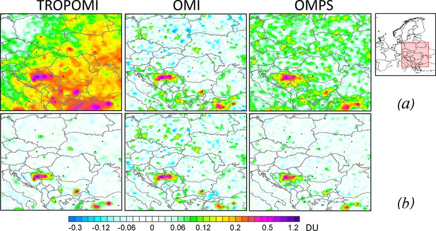
5592                                                 V. Fioletov et al.: Anthropogenic and volcanic point source SO2 emissions

   In the early 1980s, satellite measurements of backscattered        sults; however, the PCA-algorithm-based data show reduced
radiation by the Total Ozone Mapping Spectrometer (TOMS)              data scattering and smaller biases compared to the DOAS-
provided the first global estimates of SO2 from large volcanic        algorithm-based data (Fioletov et al., 2016).
eruptions (Krueger, 1983). The TOMS instrument was capa-                 The launch of the TROPOspheric Monitoring Instrument
ble of measuring backscattered solar ultraviolet (BUV) radi-          (TROPOMI) on board the Copernicus Sentinel-5 Precursor
ance at just several wavelengths. A hyperspectral instrument          in October 2017 made it possible to monitor atmospheric pol-
from the next generation (a UV–visible imaging spectrome-             lutants with an unprecedented spatial resolution, 3.5 km by
ter), the Global Ozone Monitoring Experiment (GOME) on                7 km (Veefkind et al., 2012), which is at least 12 times better
the Earth Research Satellite 2 (ERS-2), launched in 1995,             than the resolution of OMI. Since 6 August 2019, the spatial
was able to detect major anthropogenic sources (Eisinger              resolution has been further reduced in the flight direction; the
and Burrows, 1998; Khokhar et al., 2008). The launch of               TROPOMI ground pixel size is now 3.5 km by 5.5 km. It has
the Ozone Monitoring Instrument (OMI) on board NASA’s                 already been demonstrated that TROPOMI can successfully
Earth Observing System “Aura” satellite (Levelt et al., 2006,         monitor trace gases such as ozone (Garane et al., 2019), NO2
2018), with high spatial resolution of up to 13 km by 24 km           (Griffin et al., 2019), HCHO (De Smedt et al., 2018), CO
at nadir but lower at the swath edges (de Graaf et al., 2016),        (Borsdorff et al., 2019), CH4 (Hu et al., 2018), and even BrO
started a new era in satellite air-quality monitoring. Data           (Seo et al., 2019), as well as cloud properties (Loyola et al.,
from OMI, as well as from SCanning Imaging Absorp-                    2018). The operational TROPOMI SO2 retrieval algorithm
tion spectroMeter for Atmospheric CHartographY (SCIA-                 utilizes the DOAS approach (Theys et al., 2017), and early
MACHY) on the ENVISAT, the Global Ozone Monitoring                    observations demonstrated the benefits of high spatial reso-
Experiment-2 (GOME-2) on MetOp-A and MetOp-B (Cal-                    lution for monitoring volcanic plumes (Hedelt et al., 2019;
lies et al., 2000), and the Ozone Mapping and Profiler Suite          Theys et al., 2019; Queißer et al., 2019). However, these first
(OMPS) on board the NASA–NOAA Suomi National Polar-                   studies were focussed on relatively high volcanic SO2 levels.
orbiting Partnership (Suomi NPP), were used to track SO2              In this study, we perform an analysis of TROPOMI SO2 ob-
changes on the global and regional scales and estimate area           servations that include smaller anthropogenic and volcanic
and point source emissions (Carn et al., 2004, 2007; Fiole-           degassing sources. We applied a previously developed tech-
tov et al., 2013; de Foy et al., 2009; Koukouli et al., 2016a,        nique (Fioletov et al., 2015) to estimate SO2 emissions from
b; Krotkov et al., 2016; Lee et al., 2009; Li et al., 2017b;          TROPOMI observations. About 500 SO2 sources, previously
McLinden et al., 2012, 2014; Rix et al., 2012; Nowlan et              identified using OMI 2005–2015 data (Fioletov et al., 2016),
al., 2011; Thomas et al., 2005; Zhang et al., 2017). More-            were examined, and their emissions were estimated using
over, OMI measurements were used to evaluate the efficacy             TROPOMI data and then compared to emissions estimates
of cleantech solutions in reducing SO2 emissions from in-             from OMI and OMPS.
dustrial sources (Fioletov et al., 2013, 2016, 2017; Ialongo et
al., 2018; Song and Yang, 2014).
   There are two major types of UV–visible SO2 retrieval al-          2     Data sets
gorithms for nadir viewing instruments. The traditional dif-
ferential optical absorption spectroscopy (DOAS) scheme is            2.1    Satellite SO2 vertical column density data
based on the approach where absorption cross sections of rel-
evant atmospheric gases are adjusted by a non-linear least            The TROPOMI instrument on board the Sentinel-5 Precursor
squares fit procedure to the log ratio of a measured earthshine       (S5P) satellite was launched on 13 October 2017. TROPOMI
spectrum and a reference spectrum in a given wavelength in-           has the smallest spatial footprint, 3.5 km by 7 km (3.5 km
terval (Theys et al., 2015). The DOAS algorithm requires              by 5.5 km after August 2019), among the instruments of its
information about the absorption spectra of all trace gases,          class (Veefkind et al., 2012). TROPOMI measures spectra
non-elastic rotational Raman scattering (Ring effect), and in-        of backscattered solar light at 450 cross-track positions (or
strument characteristics. The uncertainties of the DOAS al-           pixels) and provides daily global coverage. TROPOMI SO2
gorithm arise from the inaccurate modelling of the various            Level 2 (/PRODUCT/sulfurdioxide_total_vertical_column)
physical processes in solar light absorption and scattering           data, processed with the S5P operational processing system
(e.g. Ring effect, surface properties), as well as artifacts in the   UPAS version 01.01.05 (Theys et al., 2017), were used in
radiance measurements (e.g. stray light, wavelength shift).           this study. In the first step of the algorithm, SO2 slant column
An alternative approach is used in the principal component            densities (SCDs), representing the effective optical-path in-
analysis (PCA) algorithm. Instead of attempting to model all          tegral of SO2 concentration, were retrieved using the DOAS
various factors other than SO2 , the PCA algorithm replaces           method. An additional background correction was applied to
them with characteristic features derived directly from the           remove possible biases in SCDs after the spectral retrieval
measurements over locations where no SO2 is expected (Li et           step. The spectral fitting was done using the 312–326 nm
al., 2013, 2017b, 2019a, b). When applied to OMI measure-             window, although two other spectral windows (325–335 nm
ments, both DOAS and PCA algorithms produce similar re-               and 360–390 nm) were used for retrievals in cases of very

Atmos. Chem. Phys., 20, 5591–5607, 2020                                                 www.atmos-chem-phys.net/20/5591/2020/

V. Fioletov et al.: Anthropogenic and volcanic point source SO2 emissions                                                      5593

high volcanic SO2 . The final product, the SO2 vertical col-        data are retrieved with the same PCA algorithm, and emis-
umn densities (VCDs), was calculated from SCDs using con-           sions estimates for the two satellite instruments are similar,
version factors (air mass factors). VCDs represent the num-         although OMPS tends to miss or underestimate emissions
ber of SO2 molecules (or total mass) in an atmospheric col-         from small sources (Zhang et al., 2017).
umn per unit area. VCDs are commonly reported in Dob-                  Suomi NPP and S5P are on the same orbit 3.5 min apart
son units (DU) where 1 DU = 2.69 × 10¹⁶ molecules cm−2 .            and cross the Equator at about 13:30 local time. Aura is on a
The standard TROPOMI SO2 data product additionally in-              similar polar orbit and crosses the Equator at about 13:45 lo-
cludes VCDs calculated for three volcanic scenarios: when           cal time. Therefore, we can assume that there is no difference
a 1 km-thick plum is located at ground level, at 7 km, and          in the measurements of the three satellite instruments related
at 15 km. In this study we focussed on anthropogenic and de-        to diurnal variations of SO2 . The TROPOMI operational SO2
gassing volcanic emissions and used only data corresponding         data record starts in April 2018. In order to have 1 full year
to ground-level plumes.                                             of data, we analyzed TROPOMI, OMI, and OMPS data for
   OMI, a Dutch–Finnish, UV–visible, wide-field-of-view,            the period from April 2018 to March 2019.
nadir-viewing spectrometer on board NASA’s Aura satellite              For emission estimates, we examined SO2 values within
was launched on 15 July 2004 (Schoeberl et al., 2006). Orig-        a 300 km radius from each emission source listed in the SO2
inally, it was able to provide daily global coverage with a         point source catalogue (Fioletov et al., 2016). There are about
resolution of up to 13 km by 24 km at nadir (de Graaf et al.,       500 sources in the catalogue; however, many sources emit-
2016; Levelt et al., 2006), but now about half of its pixels        ting SO2 in the first years of OMI operation were below the
are affected by a field-of-view blockage and stray light (the       OMI sensitivity level in 2018, either closed or now producing
so-called “row anomaly”), and SO2 cannot be retrieved suc-          substantially reduced emissions due to scrubber installation.
cessfully from those pixels. The OMI detector has 60 cross-         The most recent version of the SO2 emissions catalogue is
track positions. In our previous studies (Fioletov et al., 2016;    available from NASA’s public archive (Fioletov et al., 2019)
McLinden et al., 2016), we excluded data from the first 10          and at https://so2.gsfc.nasa.gov/measures.html (last access:
and last 10 cross-track positions from the analysis to limit        8 May 2020).
the across-track pixel width from 24 to about 40 km. How-
ever, due to row anomaly, this currently limits the number of       2.2   Air mass factors and data filtering
available pixels to 15–20. We found that excluding only the
first and the last five cross-track positions does not change the   Data filtering was applied to OMI, OMPS, and TROPOMI
emissions estimates noticeably but reduces their uncertain-         SO2 data before the analysis. The current retrieval algo-
ties, so only the first and last five pixels were excluded from     rithms are optimized for low (0.05) surface albedo; there-
the current analysis. NASA’s operational planetary bound-           fore, pixels that correspond to snow-covered high-albedo sur-
ary layer (PBL) SO2 Level 2 data product was used in this           faces were excluded from the analysis. Measurements taken
study (OMSO2; Li et al., 2019a). This data product is pro-          at high solar zenith angles (more than 70◦ ) were also ex-
duced with the principal component analysis (PCA) algo-             cluded. Only clear-sky data, defined as having a cloud radi-
rithm (Li et al., 2013, 2017). The 310.5–340 nm spectral win-       ance fraction (across each pixel) of less than 20 %, were used.
dow was used for SO2 retrievals. Detailed information on the        Negative SO2 values that were less than −3 DU were also
OMI PCA SO2 data sets and their characteristics are avail-          excluded. Values lower than the −3 DU threshold produced
able elsewhere (Krotkov et al., 2016; McLinden et al., 2015).       negative emission values in some rare cases, while higher
It should be noted that the OMI DOAS algorithm-based data           values affected the emissions estimates themselves. To elimi-
product is also available (Theys et al., 2015). While the re-       nate cases of transient volcanic SO2 , days with high volcanic
sults of the two algorithms are somewhat different, particu-        SO2 values were excluded from the analysis. If the highest
larly in large-scale biases, emissions estimates from the two       10 % of SO2 values near the analyzed site were above a cer-
algorithms demonstrate very similar results (Fioletov et al.,       tain limit on a particular day, all data from the entire day were
2016).                                                              excluded. The limit depended on the emission strength and
   The OMPS Nadir Mapper on board the Suomi National                varied from 6 DU for sources emitting less than 100 kt yr−1
Polar-orbiting Partnership (Suomi NPP) satellite operated by        to 15 DU for sources emitting > 1000 kt yr−1 (see Fioletov et
NASA and NOAA was launched in October 2011. The stan-               al., 2016, for details).
dard NASA OMPS SO2 data product (NMSO2-PCA-L2) is                      Information on air mass factors (AMFs) is required to con-
based on the same PCA algorithm as the NASA OMI data                vert TROPOMI SCDs to VCDs. AMFs depend on SO2 ver-
product (Li et al., 2019b; Zhang et al., 2017). OMPS has            tical profile shape, solar zenith angle, observation geome-
a lower spatial resolution than OMI, 50 km by 50 km, but            try, total ozone absorption, clouds, and surface reflectivity.
better signal-to-noise characteristics. OMPS SO2 VCD data           In the operational TROPOMI data set, TM5 model calcu-
are retrieved for 35 cross-track positions. Similar to OMI          lations were used to obtain a priori SO2 vertical profiles to
data analysis, large OMPS pixels at the edges of the swath          calculate AMF for each TROPOMI pixel. The model esti-
(rows < 2 or > 33) were excluded. Both OMI and OMPS SO2             mates rely on “bottom-up” emission inventories derived from

www.atmos-chem-phys.net/20/5591/2020/                                                Atmos. Chem. Phys., 20, 5591–5607, 2020
5594 V. Fioletov et al.: Anthropogenic and volcanic point source SO2 emissions
economic activity data and SO2 emissions factors for known 2.3 Wind and snow data
sources, so that in the case of a missing source in the inven-
tory, the model SO2 profile shape would be representative of The emission estimation algorithm requires wind data. As
clean background areas, causing calculated AMFs to be bi- in several previous studies (Fioletov et al., 2015; McLinden
ased high and VCDs underestimated over that source. et al., 2016), European Centre for Medium-Range Weather
The PCA algorithm uses spectrally dependent SO2 Jaco- Forecasts (ECMWF) reanalysis data (Dee et al., 2011) (http:
bians instead of AMFs. To make it consistent to the previous //apps.ecmwf.int/datasets/, last access: 8 May 2020) were ex-
operational OMI band residual difference (BRD) algorithm, tracted for every satellite pixel. Wind profiles are available
the present PCA algorithm assumes the same fixed condi- every 6 h on a 0.75◦ horizontal grid and are interpolated in
tions that correspond to typical summertime conditions in time and space to the location of each satellite pixel cen-
the eastern USA, and PCA retrievals can therefore be inter- tre. The u and v (west–east and south–north, respectively)
preted as having an effective AMF of 0.36 as in the BRD wind speed components were averaged for 1 km thick layers,
algorithm (Krotkov et al., 2006). However, a constant AMF and the winds for the layer that corresponds to the site al-
does not represent conditions such as high elevations or en- titude were used. The interactive multi-sensor snow and ice
hanced aerosol loading. As in our previous studies (Fiole- (IMS) mapping system data (Helfrich et al., 2007) were used
tov et al., 2016; McLinden et al., 2016) a single site-specific to screen out pixels over snow-covered surfaces with high
AMF was calculated for each source (McLinden et al., 2014) albedo.
and applied to both OMI/OMPS and TROPOMI estimated
emissions.
3 TROPOMI SO2
As one of the main goals of this study is to compare
TROPOMI SO2 data and emissions estimates to those from For brevity, from this point we refer to “SO2 VCD” as sim-
OMI and OMPS, we used a constant AMF of 0.36 for illus- ply “SO2 ”. It can be expected of TROPOMI that a smaller
tration maps, while for the emissions estimates we converted pixel size would yield a lower signal-to-noise level. Figure 1
TROPOMI SO2 SCDs to VCDs using the same site-specific shows the standard deviation of SO2 values at four sites, each
AMFs, thereby removing them as a potential source of vari- located at different latitudes, as a function of the TROPOMI
ability. It should be also noted that the spectral fitting win- cross-track position. The selected sites have relatively low
dow used in the TROPOMI algorithm is different from the SO2 emissions, so the standard deviations are determined
window in the PCA algorithm. However, we estimated that by the instrumental noise and possible retrieval uncertainties.
that effect is small (under 10 %) compared to other sources The standard deviations at the 20 cross-track positions at the
of uncertainties. edges of the swath are particularly high due to less across-
The SO2 absorption cross section has a moderate temper- track binning, which motivated our decision (in addition to a
ature dependence, with absorption increasing for higher tem- larger footprint) to exclude them from the analysis. There is
peratures, and there is a difference in how this dependence also a clear increase in the noise from low to high latitudes
was handled in TROPOMI and OMI/OMPS retrievals. In the with the noise standard deviations at a sub-polar site nearly
TROPOMI spectral fit, an SO2 cross section at 203 K was double compared to tropical sites. Outside the tropical belt,
used, and then the retrieved VCDs were adjusted by applying there is also some seasonality in the standard deviation val-
an AMF correction factor using temperatures from the Euro- ues, with higher values occurring in winter and lower values
pean Centre for Medium-Range Weather Forecast (ECMWF) in summer (not shown) due to weaker signals at low Sun.
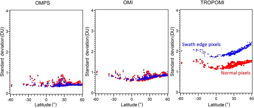
operational model (Theys et al., 2017). The OMI/OMPS The standard deviation of SO2 retrievals for the three satel-
retrieval algorithm uses the SO2 cross section at 293 K lite instruments as a function of latitude is shown in Fig. 2 for
(Krotkov et al., 2006) without any adjustment. In this work, the period from April 2018 to March 2019. The plot is based
for consistency, we used TROPOMI SO2 SCDs and con- on satellite measurements over clean areas (150–300 km dis-
verted them to VCDs using the same AMFs as we utilized tance from the catalogue source locations) and represents
for OMI and OMPS (without any temperature adjustment). background noise levels of SO2 . Large sources with annual
However, that meant that the obtained TROPOMI VCDs cor- SO2 emissions above 1000 kt yr−1 where the high standard
responded to 203 K as the original TROPOMI SCDs were deviations are likely to be influenced by the SO2 variability
calculated for that temperature. To remove the systematic itself were excluded from this analysis. Sources inside the
difference with OMI/OMPS data caused by the difference South Atlantic Anomaly (SAA) region were also excluded.
in cross-section temperature (203 K for TROPOMI vs. 293 K The standard deviations of TROPOMI data (about 1 DU over
for OMI/OMPS), we increased the TROPOMI SO2 VCDs by tropics and 1.5 DU over high latitudes) are larger than those
22 % (see Theys et al., 2017, their Fig. 6, for justification). of OMI (0.6–1 DU) and OMPS (0.3–0.4 DU) data. The stan-
dard deviations are particularly large (1.6–2.2 DU) for the
first and the last 20 pixels in the TROPOMI 450-pixels-wide
swath, which were excluded from further analysis.
Atmos. Chem. Phys., 20, 5591–5607, 2020 www.atmos-chem-phys.net/20/5591/2020/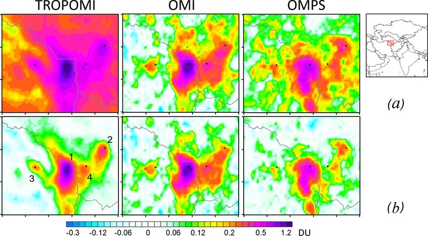
V. Fioletov et al.: Anthropogenic and volcanic point source SO2 emissions                                                            5595

Figure 1. The SO2 standard deviations as a function of the TROPOMI cross-track position (pixel number) at four sites illustrate a decline
from high to low latitudes for the period from April 2018 to March 2019. The four sites selected represent sources with very low SO2
emissions, and therefore the standard deviations represent the measurement uncertainties. The SO2 values retrieved at the first and last 20
pixels have noticeably higher standard deviations and are excluded from the analysis.

Figure 2. The OMPS, OMI, and TROPOMI SO2 standard deviation vs. latitude for “normal” (red) and “swath edge” (blue) pixels. Swath
edge pixels were defined as the first and the last 3, 5, and 20 pixels for OMPS, OMI, and TROPOMI, respectively. All other pixels were
considered normal. The plot is based on satellite measurements centred between 150 and 300 km around the sources from the catalogue. The
sources under the South Atlantic Anomaly (SAA) are excluded.

   As Fig. 2 shows, the standard deviations (σ ) for                    over the Persian Gulf, China, Mexico, and India, as well as
TROPOMI are roughly 1.5 time larger than OMI and 3 times                many anthropogenic “hotspots” such as Norilsk (Bauduin et
larger than OMPS, since the TROPOMI footprint is smaller                al., 2014; Khokhar et al., 2008) and a cluster of power plants
and each detector cell receives fewer photons than OMI and              in South Africa, and large volcanic sources such as Kilauea,
OMPS detector cells. However, the pixel size for TROPOMI                Hawai‘i, and Ambrym, Vanuatu. All three satellite data sets
is much smaller, and so the number of observations (n) over             shown in Fig. 3 do not demonstrate the large biases seen
the same area for TROPOMI is 12 and 96 times that of OMI                in the data of older versions of OMI, GOME-2, and SCIA-
and OMPS, respectively. Considering these two √   factors, and          MACHY (see Fioletov et al., 2013, their Fig. 1). Except for
assuming the standard error is proportional to σ/ n (assum-             the hotspot-affected areas, SO2 values from all three instru-
ing that the errors of individual pixels are not correlated),           ments are typically within the ±0.25 DU range. It is also in-
then the uncertainty of a TROPOMI average will be roughly               teresting to note that the South Atlantic Anomaly (SAA), an
a factor of 2 smaller than OMI and a factor of 3 smaller than           area of increased flux of energetic solar wind particles that
OMPS. In fact, due to the OMI row anomaly, the number of                may intercept instruments in low-Earth orbits such as these,
TROPOMI pixels over the same area is now a factor of 20                 significantly increases the uncertainties of OMI and OMPS
larger.                                                                 data (as well as data from GOME-2 and SCIAMACHY) but
   The global distribution of mean SO2 from TROPOMI                     has little effect on TROPOMI data.
(smoothed using oversampling techniques or pixel averaging                 There are, however, still some differences in the absolute
techniques with a 30 km radius; see e.g. Fioletov et al., 2011;         values between OMI, OMPS, and TROPOMI over some re-
Sun et al., 2018) is very similar to that from OMI and OMPS             gions. Zoomed-in plots of mean SO2 over four regions of el-
(Fig. 3). All three instruments clearly show elevated values            evated SO2 values – northern China, India, Mexico, and Iran

www.atmos-chem-phys.net/20/5591/2020/                                                     Atmos. Chem. Phys., 20, 5591–5607, 2020
5596 V. Fioletov et al.: Anthropogenic and volcanic point source SO2 emissions
different SO2 algorithms produce different biases. For exam-
ple, GOME-2 data processed with the original operational al-
gorithm (Valks and Loyola, 2009) had larger biases than the
SO2 data product based on the direct fitting method devel-
oped by the Harvard–Smithsonian Center for Astrophysics,
Cambridge, Massachusetts (Nowlan et al., 2011; see Fig. 1 in
Fioletov et al., 2013). The origin of such biases is not always
known, although an imperfect removal of the very strong
ozone absorption, which itself depends on stratospheric tem-
perature and the shape of the ozone profile, could be one of
the contributing factors.
OMI data processed with a DOAS algorithm (Theys et al.,
2015), which is similar to the present TROPOMI algorithm,
also had larger biases over some areas than those seen in the
PCA-based data (Fioletov et al., 2016). However, as was also
noted by Fioletov et al. (2016), both algorithms produce very
similar results if the large-scale biases are removed, for ex-
ample, by comparing up-wind and down-wind values around
an SO2 emissions source. In the case of large-scale biases
in an area with multiple sources, the bias can be accounted
for by introducing functions that change slowly with latitude
and longitude as suggested by Fioletov et al. (2017). This
multi-source algorithm accounts for the bias using Legen-
dre polynomials of latitude and longitude, their products, and
the emissions using functions that represent plumes from in-
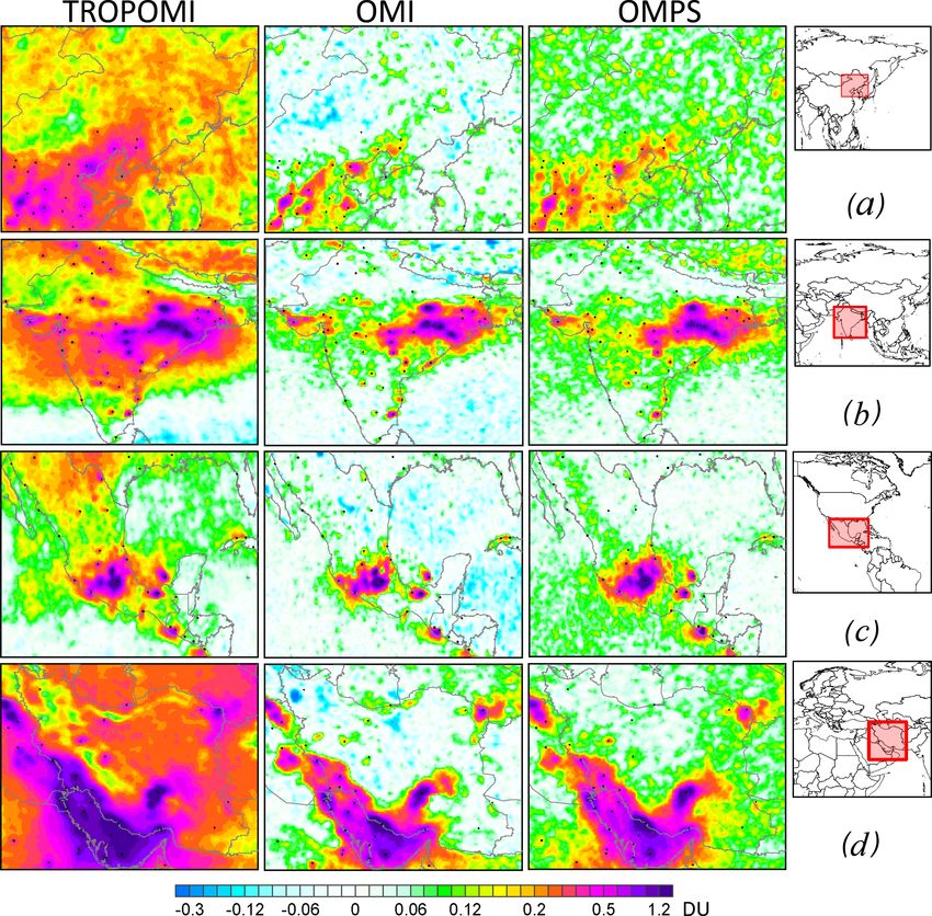
dividual sources. As an example, Fig. 5 shows original data
from TROPOMI, OMI, and OMPS over Europe and the same
data with the local biases removed using sixth-degree poly-
nomials (see Fioletov et al., 2017, for details). As Fig. 5 sug-
gests, large-scale biases seen in the original TROPOMI data
are removed by this statistical fitting procedure. Note that
OMPS data also show some large-scale biases over that re-
gion. The maps with the large-scale biases removed look very
Figure 3. Mean SO2 (DU) over the globe from TROPOMI, OMI, similar for all three satellite data sources, and all the major
and OMPS for the period from April 2018 to March 2019. Data are SO2 hotspots are clearly seen. Note that there is practically
smoothed by oversampling techniques with radius R = 30 km. The no bias in OMI data over southern Europe; hence, OMI data
area of the South Atlantic Anomaly (SAA) is left blank on the OMI with and without biases removed appear very similar.
and OMPS maps. The SAA greatly increases uncertainties of OMI
The problem of biases in TROPOMI data, as well as in the
and OMPS SO2 data but has a much smaller effect on TROPOMI
data from other satellites, requires further investigation and
SO2 data.
probably improvements of the SO2 algorithms. In the case
of TROPOMI, we saw such biases over many major areas of
interest: China, India, Europe, and the Persian Gulf. The bi-
– are shown in Fig. 4. TROPOMI SO2 means are, in gen- ases are often larger than the signals from emission sources,
eral, higher than OMI and OMPS values over these regions, which creates an impression that TROPOMI values over such
suggesting possible biases in TROPOMI data. The spatial sources are larger than those from OMI. It also appears that
scale of these biases (thousands of kilometres) is larger than the biases are larger in winter and fall than in summer and
the scale of elevated SO2 values from a typical industrial are also larger over water. It will be possible to investigate
source (100–200 km), so we will call them “large-scale bi- the time dependence of these biases as more TROPOMI data
ases”. Note that the biases are very small, only 0.1–0.2 DU; become available.
however, even such small biases could affect emissions es- As mentioned, the uncertainties of TROPOMI data aver-
timates since the SO2 enhancements from many sources are aged over a certain area are 2–3 times smaller than those of
really tiny, a few tenths of a DU. These large-scale biases OMI and OMPS. Due to its very high spatial resolution, in
are common in satellite SO2 retrievals. Their magnitude of- a single year TROPOMI can provide as much information
ten depends on the retrieval algorithm, and the same satellite on the SO2 distribution around hotspots as OMI or OMPS
measurements (i.e. calibrated Level 1B data) processed with can over several years. Figure 6 (top) shows the mean SO2
Atmos. Chem. Phys., 20, 5591–5607, 2020 www.atmos-chem-phys.net/20/5591/2020/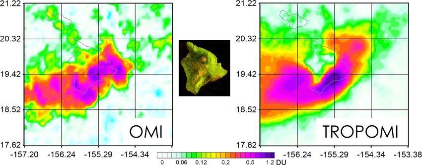
V. Fioletov et al.: Anthropogenic and volcanic point source SO2 emissions                                                          5597

Figure 4. Mean SO2 (DU) from TROPOMI, OMI, and OMPS over northern China (a), India (b), Mexico (c), and Iran (d) for the period
from April 2018 to March 2019. Large-scale biases make it difficult to interpret TROPOMI SO2 data and compare them to OMI and OMPS
data directly. Data are smoothed by oversampling techniques with R = 30 km. The black dots indicate the SO2 sources. Note that the colour
scale is different from the scale in Fig. 3.

Figure 5. TROPOMI, OMI, and OMPS mean SO2 over eastern and southern Europe for the period from April 2018 to March 2019 (a) and
the same data but with large-scale biases removed (b). Data are smoothed by oversampling/pixel averaging with R = 30 km. The black dots
indicate the SO2 emissions sources.

www.atmos-chem-phys.net/20/5591/2020/                                                    Atmos. Chem. Phys., 20, 5591–5607, 2020
5598 V. Fioletov et al.: Anthropogenic and volcanic point source SO2 emissions
over Bosnia & Herzegovina and Serbia in 2018 from OMI 4 Emissions estimates
and TROPOMI and over the 2014–2018 period from OMI,
using oversampling techniques (see Sun et al., 2018, and ref- A method developed to estimate emissions from point
erences therein). In these countries, SO2 emissions were not sources from OMI data (Fioletov et al., 2015) was applied
under the same strict emissions-cutting regulations as in EU here to TROPOMI, OMI, and OMPS data. The method is
countries. Emissions from the power plants shown in Fig. 6 based on a fit of satellite data to an empirical plume model
remained nearly constant between 2014 and 2018. A simple developed to describe the SO2 spatial distribution near emis-
version of the oversampling technique was applied, in which sion point sources. First, satellite measurements are merged
a geographical grid was established around the source and with wind data and the rotation technique is applied (Pom-
the mean value of all satellite pixels centred within a 30 km mier et al., 2013; Valin et al., 2013) so that the satellite data
radius from each grid point was calculated. As the mean is can be analyzed, assuming that the wind always has the same
calculated, the standard error of the mean can also be calcu- direction. Then, emissions and lifetimes were estimated us-
lated and used to evaluate the significance of that mean value ing the exponentially modified Gaussian fit (Beirle et al.,
by analyzing the ratio of the mean value to its standard er- 2014; Fioletov et al., 2015; de Foy et al., 2015) appropri-
ror. Figure 6 shows both the mean values (the top row) and ate for a near point source. The fitted plume model depends
the ratios (the bottom row). Although individual TROPOMI on three parameters: total mass (α) near the source; the life-
SO2 values are noisier than OMI values, the much larger vol- time or, more accurately, decay time (τ ); and the plume width
ume of TROPOMI data contributing to the mean makes it (σ ). Finally, the emission strength (E) is calculated from τ
appear less noisy than a 1-year OMI map, and only a 5-year by E = α/τ . For each source, all three parameters can be de-
OMI average demonstrates a TROPOMI-like level of noise. rived from a fit using a non-linear regression model, but when
This is further confirmed by the ratio maps (Fig. 6, bottom): doing so the uncertainties in the non-linear parameters (τ and
TROPOMI 1-year ratios are as high as 25, while OMI 1-year σ ) are often large. To minimize this uncertainty, all emissions
ratios are under 10 and only 5-year ratios are close to those were derived using a mean τ and σ , determined by averaging
for 1-year TROPOMI values. over values obtained from the non-linear fits. Thus, only one
Although averaging multiple years of OMI data can pro- parameter (α) is derived from the fit, which turns the algo-
duce the same or even higher signal-to-noise ratios as 1 year rithm into a simple linear regression model (Fioletov et al.,
of TROPOMI data, OMI cannot provide the same level of 2016).
detail as TROPOMI due to the difference in the instrument The three parameters for each of the three satellite instru-
spatial resolutions. The high spatial resolution of TROPOMI ments were estimated using April 2018–March 2019 data.
also makes it possible to see individual sources in areas It can be expected that the lifetime τ that characterizes the
where multiple sources are in close proximity. As an exam- plume decay is the same for all three instruments. Indeed,
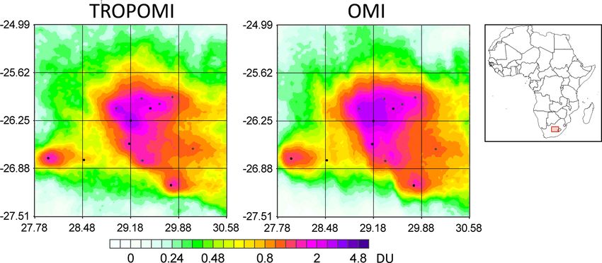
ple, Fig. 7 shows the mean SO2 over a cluster of power plants we found that the average value of τ is about 6 h for all three
in South Africa using 1 year of TROPOMI data and the en- of them. The plume width σ depends on the instrument pixel
tire (2005–2019) available record of OMI. For this plot, pixel size and is expected to be different. We estimated that, as in
averaging with a 10 km radius was used (smaller radii make the previous study (Fioletov et al., 2016), σ is about 20 km
the OMI map too noisy to see individual sources). Although for OMI. For OMPS with its larger pixels, the average σ
we used a very small radius for averaging, it is hard to distin- value is about 25 km. For TROPOMI, the average value of
guish individual sources in the OMI map, while on the 1-year σ is about 15 km. However, many SO2 sources are not re-
TROPOMI map they appear as local maxima or hotspots. ally point sources. Industrial sources are often comprised of
A high TROPOMI spatial resolution makes it possible in several individual facilities located a few kilometres apart.
some cases to resolve an individual, persistent SO2 plume. For example, in Norilsk, there are three major smelting fac-
As an example, the mean SO2 over Hawai‘i for the period tories located 8–10 km apart. For relatively large OMI pixels,
from April 2018 to March 2019 is shown in Fig. 8. The this typically does not affect σ calculations. For TROPOMI,
source, Kilauea volcano, is located at 1200 m above sea level, however, we can see that for real point sources σ is smaller,
while the mountains north and northwest of the volcano are about 10 km, than for sources with multiple facilities. Our
as high as 4000 m. The area is dominated by easterly winds. sensitivity study suggests that a change in sigma from 15
TROPOMI data demonstrate that, on average, elevated SO2 to 10 km reduces the emissions estimates by about 20 %. A
values are not observed above the volcano peak. This means better characterization of the emission sources will be re-
that the symmetrical, modified Gaussian plume model used quired in the future in order to improve emissions estimates
for emissions calculations may not describe the actual plume for sources with multiple facilities.
very well in this particular case. OMI data with their lower The calculations were performed in the same manner as
spatial resolution do not really show these features of the SO2 the original study for OMI data (Fioletov et al., 2016). The
distribution. parameter estimation was done using OMI pixels centred
within a rectangular area that spreads ±L km across the
wind direction, L km in the upwind direction and 3 · L km
Atmos. Chem. Phys., 20, 5591–5607, 2020 www.atmos-chem-phys.net/20/5591/2020/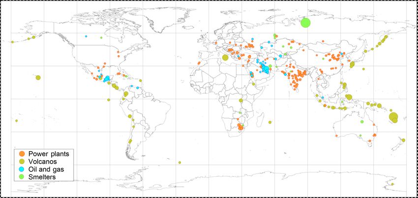
V. Fioletov et al.: Anthropogenic and volcanic point source SO2 emissions                                                        5599

Figure 6. SO2 hotspot over Serbia and Bosnia and Herzegovina: mean OMI values over a 5-year period (2014–2018) and mean OMI
and TROPOMI values over a 1-year period (from April 2018 to March 2019). Data are smoothed by oversampling/pixel averaging with
R = 30 km. The constant bias is removed. The black dots indicate the emission sources. Panels (a–c) show mean SO2 and panels (e–f) show
the ratios of the mean SO2 value to the standard error of the mean.

Figure 7. The mean TROPOMI SO2 over a cluster of power plants in South Africa for the period from April 2018 to March 2019 and
the mean 2005–2019 OMI SO2 over the same region. Data are smoothed by oversampling/pixel averaging with R = 10 km. The black dots
indicate the emission sources. Note that the colour scale is different from the scale in the previous figures.

in the downwind direction. As in the original study, the              ues have smaller uncertainties. Only pixels with associated
value of L was chosen to be 30 km for small sources (un-              wind speeds between 0.5 and 45 km h−1 were used for the
der 100 kt yr−1 ), 50 km for medium sources (between 100              fitting. The overall uncertainty of the method is about 50 %.
and 1000 kt yr−1 ), and 90 km for large sources (more than            There are several factors that contribute to the emission es-
1000 kt yr−1 ). For small sources, different L values have lit-       timate uncertainty; however, the major contributors, uncer-
tle effect on the estimated parameters, but smaller values of         tainties in AMFs and τ , appear as scaling factors that af-
L allow the separation of individual sources where multi-             fect TROPOMI-, OMI-, and OMPS-based estimates the same
ple sources are located in the same area. For larger sources,         way. To remove the local biases mentioned above, the aver-
pixels with elevated SO2 values are located over larger ar-           age SO2 VCD for the area located upwind from the source
eas, and therefore the parameters estimated for higher L val-         was calculated and then subtracted from the data. As the bi-

www.atmos-chem-phys.net/20/5591/2020/                                                  Atmos. Chem. Phys., 20, 5591–5607, 2020
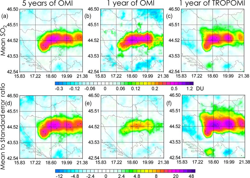
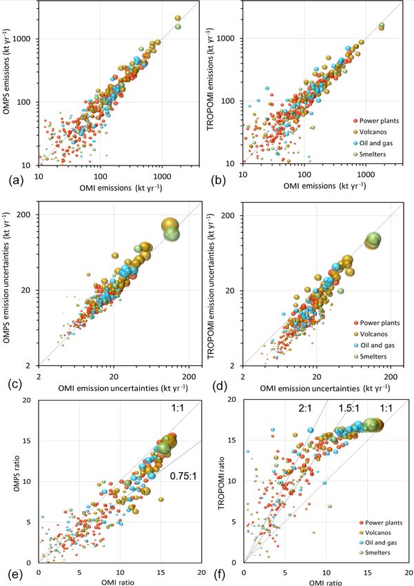
5600                                                   V. Fioletov et al.: Anthropogenic and volcanic point source SO2 emissions

Figure 8. Mean SO2 (DU) over Kilauea volcano, Hawai‘i, from OMI and TROPOMI data for the period from April 2018 to March 2019.
The volcano is in the centre of the map. The influence of orography on the SO2 distribution is clearly visible due to the high spatial resolution
of TROPOMI. A Sentinel-1 image from 23 May 2018 that illustrates the island’s orography is shown in the middle of the figure.

ases may be different from season to season, all calculations              from the three instruments). For them, the correlation coeffi-
were done for 3-month periods (seasons), and then the annual               cients are about 0.97 for both instruments. However, the cor-
emission rate was calculated by averaging seasonal emission                relation coefficient is only 0.3 if calculated just for sources
rates. Additional information about the algorithm and uncer-               that emit less than 60 kt yr−1 . There are practically no sys-
tainty analysis can be found in Fioletov et al. (2016).                    tematic biases between estimates from the three instruments.
   We examined all sources listed in the catalogue (Fioletov                  Not surprisingly, statistical uncertainties of the emissions
et al., 2016) and calculated emissions for the period from                 estimates from the three satellite instruments are also highly
April 2018 to March 2019 and their uncertainties using data                correlated (Fig. 10c and d). In general, the OMPS-based
from the three satellite instruments. It should be mentioned               emission uncertainties are slightly larger than those based on
that although the catalogue contains about 500 sources, many               OMI data. The OMI-based emission uncertainties are almost
were either closed or their emissions declined significantly               always larger than those from TROPOMI data.
due to several possible factors such as the installation of                   The relative TROPOMI emission uncertainties are lower
scrubbers and reduction in coal consumption. This includes                 than those from OMI. To illustrate that, Fig. 10e and f show
most of the sources in the USA and the European Union                      scatter plots of the ratios of their signal-to-uncertainty ra-
and many sources in China. Volcanic degassing emissions                    tios. For very large sources (> 1000 kt yr−1 ), the emission-to-
also vary with time (Carn et al., 2017), and some of the vol-              uncertainty ratio is dominated by SO2 variability and not by
canos that were active at the beginning of OMI operations                  the noise in satellite data. For example, SO2 emissions from
did not emit high amounts of SO2 in 2018–2019. Therefore,                  volcanic sources could be very different from day to day.
a decline in the number of catalogue sources detectable by                 Even if the emissions are fairly constant, different weather
TROPOMI is not entirely unexpected. The map of catalogue                   conditions (e.g. dry conditions vs. rain) affect the SO2 dis-
sources that are detectable from 1 year of TROPOMI data is                 persion patterns observed by satellites. For these very large
shown in Fig. 9. The following criteria were used to identify a            sources, such SO2 variability is larger than instrumental er-
source as detectable: (a) the source should have an emission-              rors, and the emission-to-uncertainty ratio is nearly the same
to-uncertainty ratio exceeding 5 or (b) a ratio between 3.6                for all three instruments. For smaller sources, however, mea-
and 5 but with a clear hotspot at the source with a down-                  surement uncertainties play a bigger role. For OMPS, the ra-
wind tail. There are only 20 sites in the (b) category, and                tios are mostly below the 1 : 1 line, meaning that the uncer-
we examined them on a case-by-case basis. A total of 274                   tainties of OMPS-based emissions estimates are higher than
sites – including 147 power plants, 19 smelters, 40 oil-and-               those based on OMI data. It is the opposite for TROPOMI,
gas-industry-related sources, and 68 volcanos – with annual                where the ratios are mostly above the 1 : 1 line. Moreover,
emissions from 10 to 2000 kt yr−1 that satisfy these condi-                for medium-size and small sources, the ratios group around
tions were detected. They are listed in the Supplement.                    the 1.5 : 1 and 2 : 1 lines, meaning that the TROPOMI emis-
   Scatter plots of TROPOMI-, OMI-, and OMPS-based                         sions estimate uncertainties are 1.5–2 times lower than those
emissions estimates for all SO2 catalogue sites are shown in               for OMI.
Fig. 10a and b. Emissions estimates from OMI are on the                       As all three satellite data sets can provide relatively inde-
horizontal axis of both panels. Both OMPS and TROPOMI                      pendent emissions estimates, the present satellite-based SO2
emissions estimates show a good agreement with OMI es-                     emissions inventory could be further improved by combining
timates for sources with estimated emissions above 50–                     emissions estimates from the three sources. Due to its high
60 kt yr−1 (calculated as an average of emissions estimates                resolution, and hence lower detection limit, TROPOMI can

Atmos. Chem. Phys., 20, 5591–5607, 2020                                                       www.atmos-chem-phys.net/20/5591/2020/
V. Fioletov et al.: Anthropogenic and volcanic point source SO2 emissions                                                              5601

Figure 9. SO2 emissions sources seen by TROPOMI in 2018. We checked ∼ 500 locations where OMI detected SO2 emissions between
2005 and 2014 (Fioletov et al., 2016). Note that some of them are not active now or have had their emissions significantly reduced. TROPOMI
can “see” 278 sites, including 150 power plants, 19 smelters, 41 oil-and-gas-industry-related sources, and 68 volcanos, with annual emissions
from 10 to 2000 kt. The size of the symbols is proportional to the annual emission values.

potentially identify many more sources than OMI and OMPS                 5   Summary and discussion
and then obtain emissions estimates for them. An exhaustive
analysis of this is beyond the scope of this paper. However, as
an example of the sizable advantage offered by TROPOMI,                  The first analysis of TROPOMI near-surface SO2 for the pe-
Fig. 11 shows the mean TROPOMI SO2 distribution (from                    riod from April 2018 to March 2019 reveals global distri-
April 2018 to March 2019) at the border between Iran and                 butions and features very similar to those seen from OMI
Turkmenistan. The biggest source is the Khangiran gas re-                and OMPS: elevated values over the Persian Gulf, India,
finery (1), an Iranian source that is included in the cata-              and China; major hotspots over Norilsk, Russia, and South
logue. The second largest source is located near Mary, Turk-             Africa; and major persistent volcanic sources such as Ki-
menistan (2), and is related to gas exploration. The LAND-               lauea, Hawai‘i, and Ambrym, Vanuatu. Outside the areas
SAT satellite images show that the source was built from                 affected by these hotspots, all three instruments typically
2012 to 2014. While 1 year of OMI data shows a signal                    demonstrate low background SO2 values within ±0.25 DU.
from that region, they can hardly point to the source location.             Over clean areas, the spatial standard deviations of
TROPOMI data clearly show a hotspot in both mean SO2 (as                 TROPOMI data (about 1 DU over tropics and 1.5 DU over
shown) and the high signal-to-noise ratio (not shown) right              high latitudes) are larger than those of OMI (0.6–1 DU) and
at the source location. Moreover, there are two other sources            OMPS (0.3–0.4 DU) data. However, despite higher uncer-
that can be resolved by TROPOMI. One of them, located east               tainties of individual TROPOMI pixels, spatially averaged
of Khangiran, could be related to two power plants (Toos                 TROPOMI data over respective field of views have uncer-
and Ferdosi (3)) that are 1 km apart. This source can also be            tainties that are 2–3 times smaller than those from OMI and
used as an illustration of the difference in emission uncertain-         OMPS data. As a result, annual mean SO2 maps smoothed
ties between TROPOMI and OMI/OMPS. TROPOMI-based                         by spatial filtering appear less noisy than corresponding
emissions estimates for this source are 14 kt yr−1 with the              OMI maps. In terms of the signal-to-noise ratio, 1 year of
standard error of 2.8 kt yr−1 , 5 times lower than the emis-             TROPOMI smoothed mean values has the same uncertain-
sion strength itself. The standard errors of OMI- and OMPS-              ties as 4–5 years of smoothed mean values based on OMI
based emissions estimates are 6.1 and 7.1 kt yr−1 , respec-              data.
tively, which is 2–3 times that of TROPOMI.                                 We tested about 500 SO2 sources previously detected
                                                                         from OMI data from 2005 to 2015; however, many of these
                                                                         sources emitted much less SO2 in 2018 and 2019 than at the
                                                                         beginning of OMI operation. That includes, for example, al-

www.atmos-chem-phys.net/20/5591/2020/                                                      Atmos. Chem. Phys., 20, 5591–5607, 2020
5602 V. Fioletov et al.: Anthropogenic and volcanic point source SO2 emissions Figure 10. (a) Estimated OMI-, OMPS-, and TROPOMI-based emissions in kilotons per year. The bubble area is proportional to the ratio of emission to uncertainty. The bigger the bubble, the more reliable the estimate. (b) Emission uncertainties in kilotons per year. The bubble area is proportional to the emission rate. The bigger the bubble, the higher the emissions. (c) Ratios between estimated emissions and their uncertainties. The bubble area is proportional to the emission rate. most all US sources and many sources in Europe and China. account that the number of useful TROPOMI pixels is about We were able to identify 274 sources where annual (from 20 times higher than that of OMI. If the statistical uncertain- April 2018 to March 2019) emissions can be estimated from ties are inversely proportional to the square root of the num- TROPOMI data. Their emissions are in the range from 10 to ber of averaged pixels and their uncertainties are the same, 2000 kt yr−1 . then it is expected that the standard errors for TROPOMI Currently TROPOMI is able to provide point source SO2 emissions estimates should be about 4–5 times lower than emissions estimates that have 1.5–2 times lower uncertainties those for OMI. Taking into account that the SO2 uncertain- than those from OMI, but it is less than expected, taking into ties of individual TROPOMI pixels are 1.5–2 times larger Atmos. Chem. Phys., 20, 5591–5607, 2020 www.atmos-chem-phys.net/20/5591/2020/
V. Fioletov et al.: Anthropogenic and volcanic point source SO2 emissions                                                              5603

Figure 11. TROPOMI, OMI and OMPS mean SO2 (DU) over the Khangiran region for the period from April 2018 to March 2019 (a). The
same data, but with large-scale biases removed (b). Data are smoothed by oversampling/pixels averaging with R = 20 km. The black dots
indicate the SO2 emissions sources: gas refinery at Khangiran, Iran (1); gas exploration sources at Mary (2) and Sovetabad (4), Turkmenistan;
Toos and Ferdosi power plants, Iran (3).

than those of OMI pixels, one can expect that TROPOMI                    with smaller biases and lower noise than the present opera-
emission uncertainties would be 2.5–3.3 times lower than                 tional algorithm. Such an improved algorithm is now under
OMI emission uncertainties, which is higher than the values              development. Preliminary TROPOMI SO2 retrieval tests ap-
of 1.5–2 that we derived directly from emissions estimates.              plying a PCA-based algorithm have shown some promise,
This may suggest that errors in individual TROPOMI pixels                and work is underway to better understand algorithmic dif-
are correlated, for example, due to large-scale biases.                  ferences between DOAS and PCA.
   There are larger-scale spatial biases in TROPOMI data
over some areas that appear to be larger than similar biases in
OMI and OMPS data. While the absolute magnitude of the                   Data availability. OMI and OMPS PCA SO2 data used in
biases is not very large (0.1–0.2 DU), it can be comparable              this study have been publicly released as part of the Aura
to the SO2 enhancements over large sources. Due to these                 OMI Sulfur Dioxide Data Product (OMSO2) and can be
biases, SO2 values over some sources may appear larger in                obtained free of charge from the Goddard Earth Sciences
                                                                         (GES) Data and Information Services Center (Li et al., 2019a,
TROPOMI data than in OMI and OMPS data. If, however,
                                                                         https://doi.org/10.5067/Aura/OMI/DATA2022; Li et al., 2019b,
such biases are removed by, for example, a statistical fit-              https://doi.org/10.5067/MEASURES/SO2/DATA203). TROPOMI
ting procedure, TROPOMI annual mean SO2 maps are very                    data are freely available from the European Union Copernicus
similar to OMI and OMPS maps. It also appears that these                 Sentinel-5P data hub (https://s5phub.copernicus.eu (ESA, 2020);
TROPOMI biases have a larger amplitude in winter and fall,               http://www.tropomi.eu, last access: 8 May 2020).
although it is hard to say that this is a repeatable seasonal
effect based on just 1 year of data.
   Biases are very common in early versions of all satellite             Supplement. The supplement related to this article is available on-
SO2 products, and currently their origin is still not com-               line at: https://doi.org/10.5194/acp-20-5591-2020-supplement.
pletely clear. The very small SO2 absorption signal in the
UV needs to be detected against a large contribution from
ozone absorption. The latter is a strong function of strato-             Author contributions. VF analyzed the data and prepared the paper
spheric temperature (and hence ozone profile). Any imper-                with substantial input from CM and critical feedback from all the
fection in any of these parameters may yield a bias in re-               co-authors. CM and DG generated the TROPOMI, OMPS, and OMI
trieved SO2 . This, however, does not explain biases in the              data subsets for the analysis. NT, DGL, and PH provided TROPOMI
                                                                         data products. CL and NK provided OMI and OMPS data products.
tropical region where ozone variability is low. Development
of a PCA-type algorithm for TROPOMI could help to re-
duce these biases and improve the overall quality of the data.
                                                                         Competing interests. The authors declare that they have no conflict
An improved version of the TROPOMI processing algorithm
                                                                         of interest.
that includes a PCA component may produce a data product

www.atmos-chem-phys.net/20/5591/2020/                                                      Atmos. Chem. Phys., 20, 5591–5607, 2020
5604 V. Fioletov et al.: Anthropogenic and volcanic point source SO2 emissions
Special issue statement. This article is part of the special is- Bauer, P., Bechtold, P., Beljaars, A. C. M., Berg, L. van de, Bid-
sue “TROPOMI on Sentinel-5 Precursor: first year in operation lot, J., Bormann, N., Delsol, C., Dragani, R., Fuentes, M., Geer,
(AMT/ACP inter-journal SI)”. It is not associated with a confer- A. J., Haimberger, L., Healy, S. B., Hersbach, H., Hólm, E. V.,
ence. Isaksen, L., Kållberg, P., Köhler, M., Matricardi, M., McNally,
A. P., Monge-Sanz, B. M., Morcrette, J.-J., Park, B.-K., Peubey,
C., Rosnay, P. de, Tavolato, C., Thépaut, J.-N., and Vitart, F.: The
Acknowledgements. We acknowledge the NASA Earth Science Di- ERA-Interim reanalysis: Configuration and performance of the
vision for funding OMI and OMPS SO2 product development and data assimilation system, Q. J. Roy. Meteorol. Soc., 137, 553–
analysis. The Dutch- and Finnish-built OMI instrument is part of 597, https://doi.org/10.1002/qj.828, 2011.
the NASA EOS Aura satellite payload. The OMI project is man- de Foy, B., Lu, Z., Streets, D. G., Lamsal, L. N., and Duncan,
aged by the Netherlands Royal Meteorological Institute (KNMI). B. N.: Estimates of power plant NOx emissions and lifetimes
The KNMI activities for OMI are funded by the Netherlands Space from OMI NO2 satellite retrievals, Atmos. Environ., 116, 1–11,
Office. This paper contains modified Copernicus Sentinel data. We https://doi.org/10.1016/j.atmosenv.2015.05.056, 2015.
acknowledge financial support from DLR programmatic (S5P KTR de Graaf, M., Sihler, H., Tilstra, L. G., and Stammes, P.: How
2472046) for the development of TROPOMI retrieval algorithms. big is an OMI pixel?, Atmos. Meas. Tech., 9, 3607–3618,
The Sentinel-5 Precursor TROPOMI Level 1 and Level 2 products https://doi.org/10.5194/amt-9-3607-2016, 2016.
are processed at DLR with funding from the European Union (EU) De Smedt, I., Theys, N., Yu, H., Danckaert, T., Lerot, C., Comper-
and the European Space Agency (ESA). Nicolas Theys acknowl- nolle, S., Van Roozendael, M., Richter, A., Hilboll, A., Peters,
edges financial support from the ESA S5P MPC (4000117151/16/I- E., Pedergnana, M., Loyola, D., Beirle, S., Wagner, T., Eskes, H.,
LG) and Belgium Prodex TRACE-S5P (PEA 4000105598) projects. van Geffen, J., Boersma, K. F., and Veefkind, P.: Algorithm theo-
retical baseline for formaldehyde retrievals from S5P TROPOMI
and from the QA4ECV project, Atmos. Meas. Tech., 11, 2395–
Review statement. This paper was edited by Ilse Aben and re- 2426, https://doi.org/10.5194/amt-11-2395-2018, 2018.
viewed by two anonymous referees. Eisinger, M. and Burrows, J. P.: Tropospheric sulfur dioxide ob-
served by the ERS-2 GOME instrument, Geophys. Res. Lett.,
25, 4177–4180, 1998.
ESA: TROPOMI SO2 data, available at: https://s5phub.copernicus.
References eu, last access: 8 May 2020.
Fioletov, V. E., McLinden, C. A., Krotkov, N., Moran, M.
Bauduin, S., Clarisse, L., Clerbaux, C., Hurtmans, , and Coheur, D., and Yang, K.: Estimation of SO2 emissions us-
P.-F., IASI observations of sulfur dioxide (SO2 ) in the bound- ing OMI retrievals, Geophys. Res. Lett., 38, L21811,
ary layer of Norilsk, J. Geophys. Res. Atmos., 119, 4253–4263, https://doi.org/10.1029/2011GL049402, 2011.
https://doi.org/10.1002/2013JD021405, 2014. Fioletov, V. E., McLinden, C. A., Krotkov, N., Yang, K., Loyola,
Beirle, S., Hörmann, C., Penning de Vries, M., Dörner, S., Kern, D. G., Valks, P., Theys, N., Van Roozendael, M., Nowlan, C. R.,
C., and Wagner, T.: Estimating the volcanic emission rate and Chance, K., Liu, X., Lee, C., and Martin, R. V.: Application of
atmospheric lifetime of SO2 from space: a case study for OMI, SCIAMACHY, and GOME-2 satellite SO2 retrievals for
Kı̄lauea volcano, Hawai‘i, Atmos. Chem. Phys., 14, 8309–8322, detection of large emission sources, J. Geophys. Res.-Atmos.,
https://doi.org/10.5194/acp-14-8309-2014, 2014. 118, 11399–11418, https://doi.org/10.1002/jgrd.50826, 2013.
Borsdorff, T., aan de Brugh, J., Pandey, S., Hasekamp, O., Aben, Fioletov, V. E., McLinden, C. A., Krotkov, N. A., and Li,
I., Houweling, S., and Landgraf, J.: Carbon monoxide air pollu- C.: Lifetimes and emissions of SO2 from point sources
tion on sub-city scales and along arterial roads detected by the estimated from OMI, Geophys. Res. Lett., 42, 1–8,
Tropospheric Monitoring Instrument, Atmos. Chem. Phys., 19, https://doi.org/10.1002/2015GL063148, 2015.
3579–3588, https://doi.org/10.5194/acp-19-3579-2019, 2019. Fioletov, V. E., McLinden, C. A., Krotkov, N., Li, C., Joiner, J.,
Callies, J., Corpaccioli, E., Eisinger, M., Hahne, A., and Lefebvre, Theys, N., Carn, S., and Moran, M. D.: A global catalogue
A.: GOME-2-Metop’s second-generation sensor for operational of large SO2 sources and emissions derived from the Ozone
ozone monitoring, ESA Bull., 102, 28–36, 2000. Monitoring Instrument, Atmos. Chem. Phys., 16, 11497–11519,
Carn, S. A., Krueger, A. J., Krotkov, N. A., and Gray, M. https://doi.org/10.5194/acp-16-11497-2016, 2016.
A.: Fire at Iraqi sulfur plant emits SO2 clouds detected Fioletov, V., McLinden, C. A., Kharol, S. K., Krotkov, N. A., Li,
by Earth Probe TOMS, Geophys. Res. Lett., 31, L19105, C., Joiner, J., Moran, M. D., Vet, R., Visschedijk, A. J. H., and
https://doi.org/10.1029/2004GL020719, 2004. Denier van der Gon, H. A. C.: Multi-source SO2 emission re-
Carn, S. A., Krueger, A. J., Krotkov, N. A., Yang, K., and Levelt, P. trievals and consistency of satellite and surface measurements
F.: Sulfur dioxide emissions from Peruvian copper smelters de- with reported emissions, Atmos. Chem. Phys., 17, 12597–12616,
tected by the Ozone Monitoring Instrument, Geophys. Res. Lett., https://doi.org/10.5194/acp-17-12597-2017, 2017.
34, L09801, https://doi.org/10.1029/2006GL029020, 2007. Fioletov, V., McLinden, C., Krotkov, N., Li, C., Leonard, P.,
Carn, S. A., Fioletov, V. E., McLinden, C. A., Li, C., Joiner, J., and Carn, S.: Multi-Satellite Air Quality Sulfur
and Krotkov, N. A.: A decade of global volcanic SO2 Dioxide (SO2 ) Database Long-Term L4 Global V1, edited
emissions measured from space, Sci. Rep.-UK, 7, 44095, by: Leonard, P., Greenbelt, MD, USA, Goddard Earth Sci-
https://doi.org/10.1038/srep44095, 2017. ence Data and Information Services Center (GES DISC),
Dee, D. P., Uppala, S. M., Simmons, A. J., Berrisford, Poli, P., https://doi.org/10.5067/MEASURES/SO2/DATA403, 2019.
Kobayashi, S., Andrae, U., Balmaseda, M. A., Balsamo, G.,
Atmos. Chem. Phys., 20, 5591–5607, 2020 www.atmos-chem-phys.net/20/5591/2020/You can also read