Financial Impacts of Road User Charges on Urban and Rural Households - EBP | US
←
→
Page content transcription
If your browser does not render page correctly, please read the page content below

f

            Financial Impacts of
          Road User Charges on
    Urban and Rural Households

         Prepared for:
         Western Road User Charge Consortium (RUC West)

         In cooperation with
         Oregon Department of Transportation
         355 Capitol Street NE, MS 11, Salem, OR 97301-3871

         Prepared by:
         Economic Development Research Group, Inc.
         155 Federal Street, Suite 600, Boston, MA 02110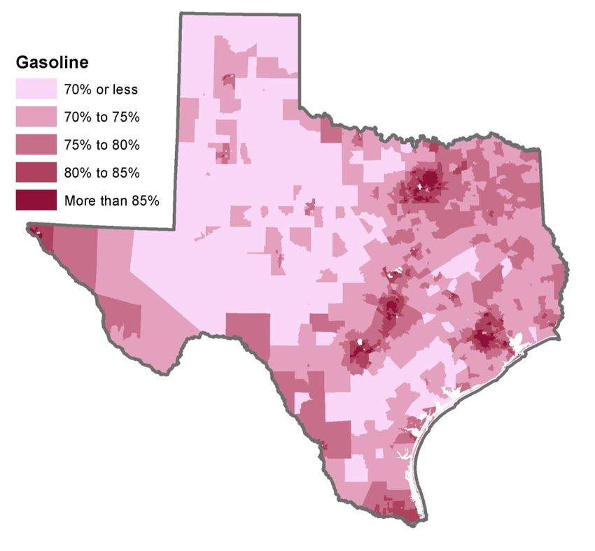
TABLE OF CONTENTS
Introduction ...................................................................................................................................... 1
Chapter 1: Estimates of Annual VMT by Non-gasoline-powered Vehicles (Task 3) ............................... 2
       VMT Estimates ................................................................................................................................. 3
       Comparisons to Other Data Sources................................................................................................ 4
       Fuel Mix Analysis.............................................................................................................................. 6
       Summary .......................................................................................................................................... 7
Chapter 2: Urban, Mixed, and Rural Data Analysis (Task 4) .................................................................. 8
       Travel Estimates to Be Used in Financial Analysis ........................................................................... 8
       Vehicle Characteristics for the Urban, Mixed, and Rural Portions of Project States ..................... 12
       Differences in Travel Patterns for Urban and Rural Households ................................................... 13
       Summary ........................................................................................................................................ 16
Chapter 3: Financial Impacts to Systems (Task 5)............................................................................... 17
Chapter 4: Documentation For Analysis (Task 6) and Tool (Task 8) .................................................... 20
       Workbook Tool Overview .............................................................................................................. 20
       Tool Description ............................................................................................................................. 21
       Structural Differences Between the Tool and Completed Study ................................................... 21
       Input Data ...................................................................................................................................... 22
       Data Sources .................................................................................................................................. 27
       Results Description ........................................................................................................................ 28
Appendix A: Task 2 Memo ................................................................................................................ 32
      Addendum to Task 2 Memo........................................................................................................... 36
Appendix B: Percentage of Annual Vehicle Miles Traveled by Fuel Type ............................................ 37
Appendix C: Changes in Household Costs Under a Revenue Neutral RUC ........................................... 51
      Arizona ........................................................................................................................................... 51
      California ........................................................................................................................................ 52
      Idaho .............................................................................................................................................. 53
      Montana......................................................................................................................................... 54
      Oregon ........................................................................................................................................... 55
      Texas .............................................................................................................................................. 56
      Utah ............................................................................................................................................... 57
      Washington .................................................................................................................................... 58
Appendix D: Vehicles ....................................................................................................................... 59
      The Importance of Prioritizing ....................................................................................................... 59
      Identifying Vehicle Types for Exclusion ......................................................................................... 60
      Standardizing and Leveraging Multiple Databases ........................................................................ 61
Appendix E: Code ............................................................................................................................. 62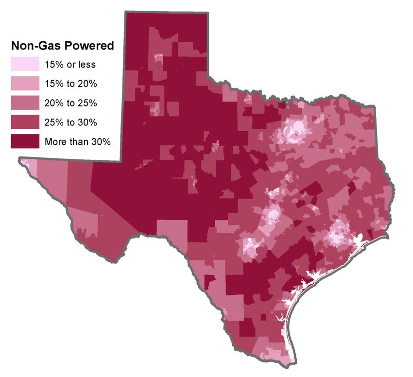
LIST OF TABLES
Table 1. Estimates of Total Annual VMT, Non-Gas VMT, and Non-Gas Percent of VMT for the Participating
States ............................................................................................................................................................ 2
Table 2. Annual VMT by Type of Non-Gasoline Fuel for the Participating States (in Millions) .................... 3
Table 3. Percent VMT by Type of Non-Gasoline Fuel for the Participating States ....................................... 3
Table 4. Daily Household Vehicle Miles Traveled Estimates for the Participating States ............................ 4
Table 5. Comparison of Statewide Total Daily Vehicle Miles Traveled for California Using Different Data
Sources .......................................................................................................................................................... 5
Table 6. Universe of Registration Records Used in Fuel Mix Analysis and Four Causes for Difference
between Vehicle Records Received and Vehicles Contained in Final Analysis Dataset ............................... 6
Table 7. Percent of Vehicles by Fuel Type for the Participating States ........................................................ 7
Table 8. Count of Vehicles by Fuel Type for the Participating States ........................................................... 7
Table 9. Estimate of Household Annual VMT in Millions Subject to the Gasoline Tax (Gasoline, Hybrid, 50%
of Flex/Biofuel).............................................................................................................................................. 8
Table 10. Estimate of Additional Household Annual VMT in Millions Subject to the Road Usage Charge
(Electric, Hydrogen, and 50% of Flex/Bio Fuel)............................................................................................. 9
Table 11. Percent Non-Gasoline-Powered VMT by Urban, Mixed, and Rural Portions of States, when
Classified by Census Tracts ......................................................................................................................... 12
Table 12. Average Fuel Efficiency for Vehicles in Urban, Mixed, and Rural Census Tracts of Project States –
Gas-Taxed Vehicles Only ............................................................................................................................. 12
Table 13. Average Vehicle Age for Vehicles in Urban, Mixed, and Rural Census Tracts of Project States . 13
Table 14. Analysis of Urban versus Rural Trip Frequency and Length for Various Purposes in the NHTS . 13
Table 15. Analysis of Urban versus Rural Trip Frequency and Length for Various Purposes in the OHAS . 13
Table 16. Daily Vehicle Miles of Travel (DVMT) from Household Travel Surveys....................................... 14
Table 17. Daily VMT per Household in Urban, Mixed, and Rural Tracts, based on EDR Group Estimates . 15
Table 18. Daily Trips per Household in Urban, Mixed, and Rural Tracts, based on EDR Group Estimates 15
Table 19. Average Trip Length for Residents of Urban, Mixed, and Rural Tracts, based on EDR Group
Estimates ..................................................................................................................................................... 16
Table 20. Reduction in Payments Under RUC Compared to a Gas Tax ...................................................... 17
Table 21. Gasoline Tax Paid Minus Road Usage Charge Paid by Urban-Mixed-Rural Regions ($)* ............ 18
Table 22. Comparisons of Gas Tax and Road Usage Charge Rates for Participating States ....................... 18
Table 23. Estimated Gas Tax Paid by In-Study Vehicles in Urban-Mixed-Rural Portions of States ............ 19
Table 24. Estimated Road Usage Charge Paid by In-Study Vehicles in Urban-Mixed-Rural Portions of States
at an Equivalent Rate .................................................................................................................................. 19
Table A-25. The 10 Primary RUCA Codes .................................................................................................... 32
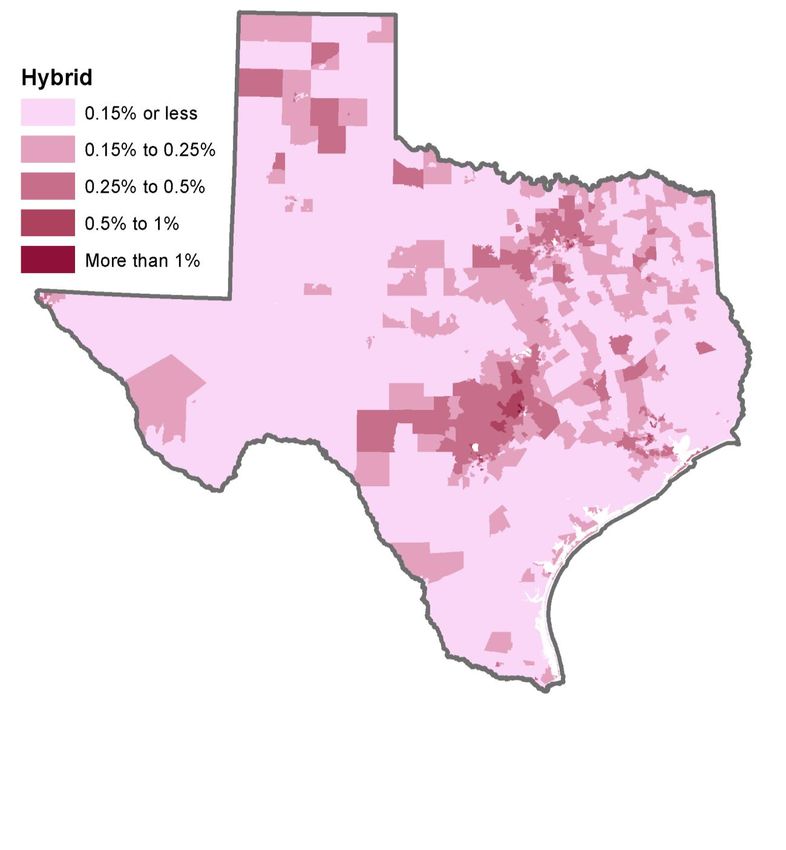
Table A-26. Adopted Aggregation to Urban-Mixed-Rural Classes with Summary Statistics for the Eight-
State Region ................................................................................................................................................ 33

LIST OF FIGURES
Figure 1. Selection of non-public streets longer than 200 meters in Oregon using the ESRI StreetsMap NA
Layer............................................................................................................................................................ 10
Figure 2. Selection of non-public streets longer than 200 meters in North-Central Utah using the ESRI
StreetsMap NA layer ................................................................................................................................... 11
Figure 3. Unequal Returns to Time and Effort ............................................................................................ 59
Figure 4. Vehicle Type Classes in Source Data ............................................................................................ 60
INTRODUCTION
This report provides a discussion, documentation and references to the sources of data used to develop
an analysis of the financial impacts of a revenue-neutral road user charge (RUC) for drivers in urban and
rural counties for eight states in the Western Road Usage Charge Consortium (WRUCC). The analysis
conducted for this study was applied uniformly to all eight participating states so that a clearer and more
comprehensive assessment of the impact of RUCs could be developed, and so that any differences in
financial impact on a state-by-state basis could be understood in the context of a consistent
methodological approach.
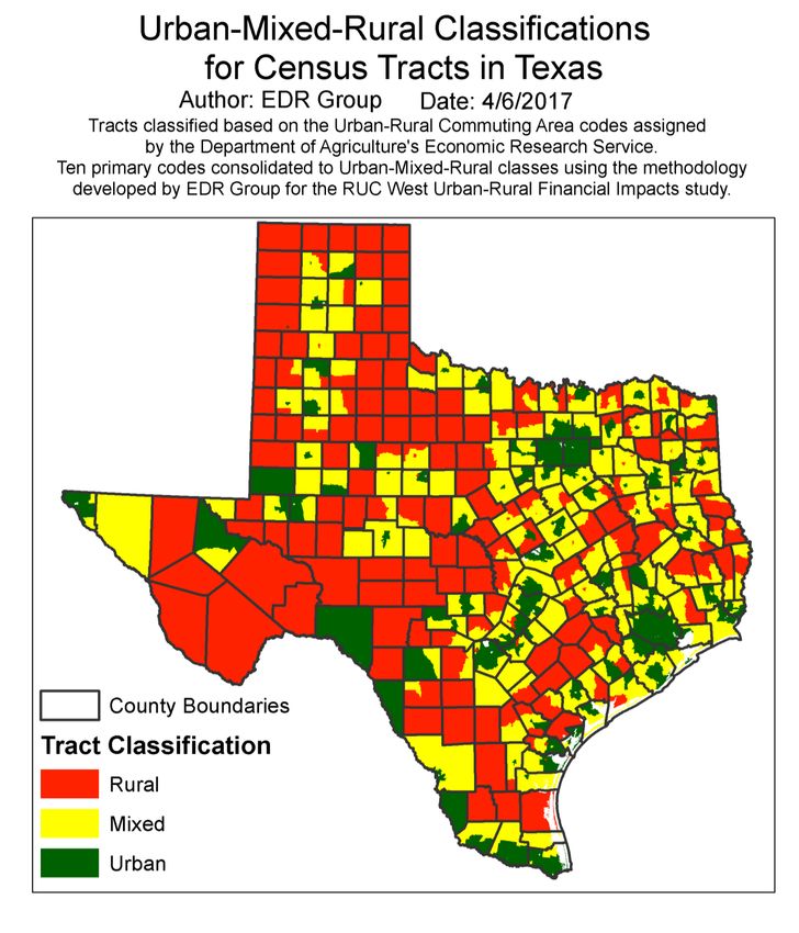
Initial criteria for categorizing counties into those with either urban or rural characteristics were
developed as part of a separate memorandum to the WRUCC’s Project Advisory Committee (PAC). In that
memorandum, the study team recommended that subsequent analysis be focused at the census tract
level and that census tracts be designated as urban, rural or mixed to fully reflect the variation in travel
characteristics for some of the larger, more diverse counties that characterize the member states. This
recommendation was accepted, and all subsequent analysis was conducted using census tract-based
information. Final tabulations in this report are provided on a state-wide basis with detailed information
displayed at the census tract level.
The report is organized so that the chapters correspond to each of the key tasks required for the study.
Chapter 1 presents the estimates of annual vehicle miles traveled (VMT) by non-gasoline powered vehicles
(Task 3), Chapter 2 identifies the costs borne by each urban, mixed and rural census tract in each of the
states (Task 4), and Chapter 3 provides an estimate of the financial impacts to households in urban, rural
and mixed census tracts in each of the states (Task 5). Chapter 4 documents the methods used for the
study and how they were incorporated in the tool (Tasks 6 and 8).
Key Assumptions of this Analysis
• Financial impacts are measured at the place of household residences, which are categories
as urban, mixed and rural at a census tract level of geography
• State vehicle registration data is a key component of this analysis
• Other data sources are from national, publicly-available sources to allow consistency across
all eight states and reproducibility.
• All relevant vehicles are registered at the place of household residence
• Only on-commercial household vehicles are included, with diesel and non-gasoline fossil
fuels excluded.
• RUC rate tested is revenue neutral on a statewide basis for studied population
There are five appendices included with this report. Appendix A documents the urban-rural classification
scheme developed for Task 2, via the memo delivered during that stage of the project. Appendix B shows
census tract detail on a state-by-state basis showing the percent of census tract VMT by state for each
fuel type assessed in the study. Appendix C shows the percentage increase or decrease in costs under a
revenue neutral RUC by census tract for each of the participating states. Appendix D discusses details of
the vehicle registration decoding, while Appendix E provides the VBA code used by the tool delivered.
Data on vehicle registration information used in this report was provided with the cooperation of the
participating states. A computer-based system to replicate this analysis is being provided as a separate
work product so that other members of the WRUCC can replicate the analysis. The study team sincerely
appreciates the cooperation and feedback from each of the participating states in developing the data
used in this report.
Financial Impacts of RUC Drivers in Rural and Urban Counties 1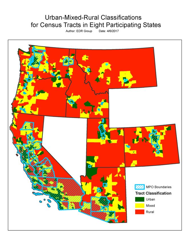
CHAPTER 1: ESTIMATES OF ANNUAL VMT BY NON-
GASOLINE-POWERED VEHICLES (TASK 3)

This section of the report describes the basis for estimates of the annual vehicle miles traveled (VMT) by
non-gasoline powered and hybrid passenger vehicles for each of the states that provided data for this
study. An estimate of annual non-gasoline-powered vehicle miles traveled (VMT) for each state is
necessary to calculate accurate per-vehicle expenditures based on the current gas tax and a Road User
Charge (RUC) alternative. This is important as some vehicles are currently paying little or no gas tax
(depending on the type of vehicle) and will begin to pay a full share of costs currently covered by the gas
tax under a RUC, while other vehicles (e.g., diesel-powered vehicles) will continue to pay a different type
of tax. EDR Group has developed estimates of VMT for gas and non-gas powered vehicles as shown in
Table 1. Appendix B shows the distribution of VMT associated with different fuel types across the
participating states, with separate maps for the initial seven states completed and for Texas.
Non-gasoline-powered VMT is estimated by combining two lines of analysis. First, VMT is estimated for
each census tract in the participating states using household characteristics. Second, fuel type mixes are
estimated at the lowest geographic level possible with the vehicle registration data provided by the states.
These estimates are combined to estimate fuel type shares of VMT in each tract. Vehicle use is assumed
to be independent of vehicle fuel type, such that a gasoline-powered car and an electric car travel the
same mileage per year. The following sections explain the estimation methodology and are designed to
be used to produce a similar analysis for non-participating states. Table 1 shows the total estimated VMT
in each participating state, the total estimated non-gasoline VMT, and the share of total VMTs attributable
to non-gasoline powered vehicles.

Table 1. Estimates of Total Annual VMT, Non-Gas VMT, and Non-Gas Percent of VMT for the
Participating States
                                       Total VMT                 Non-Gasoline VMT                Non-Gasoline
            State                       (Billions)                   (Billions)                 Percent of Total
    Arizona                                        26,771                        2,657                           9.9%
    California                                    155,826                        7,542                           4.8%
    Idaho                                           7,800                          643                           8.2%
    Montana                                         5,152                        1,046                          20.3%
    Oregon                                         17,329                        2,262                          13.1%
    Texas                                         130,396                       24,841                          19.1%
    Utah                                           12,633                        1,877                          14.9%
    Washington                                     32,205                        2,476                           7.7%
Montana and Texas show the highest non-gasoline-powered share of VMT in Table 1. Oregon and Utah
also show considerable penetration of other fuel technology. Table 2 and Table 3 provide VMT counts and
percentages, respectively, that are attributable to electric, hybrid, flex fuel and biofuel1, diesel, and
alternative fossil fuels categories of non-gasoline-powered VMT. This information helps understand the
nuances driving the results in Table 1. High shares of non-gasoline powered VMT in Montana are largely
driven by a much higher percent of diesel in the registration data. Texas has by far the highest flex/biofuel

1
 Flex fuel and biofuel vehicles are those which can operate some of the time or all of the time using biofuel mixes
that are unsuitable for standard vehicles. A significant portion of gasoline sold in the United States contains up to 10
percent ethanol and most gasoline combustion engines can safely operate with up to 15 percent ethanol content.
Financial Impacts of RUC Drivers in Rural and Urban Counties                                                            2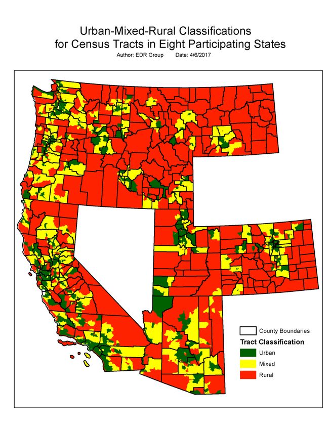
and other fossil fuel penetrations. Oregon has the highest penetration of hybrid vehicles. Oregon and
Utah also have higher than average diesel-powered VMT.

Table 2. Annual VMT by Type of Non-Gasoline Fuel for the Participating States (in Millions)
                            Electric/                          Flex fuel/                                             Total
          State            Hydrogen            Hybrid           Biofuel        Other Fossil         Diesel           Non-Gas
    Arizona                        20.3            514.0           1,794.9              3.9             323.7           2,656.7
    California                   605.5           3,216.4           1,937.1            117.2           1,665.9           7,542.0
    Idaho                           1.1             67.4             395.3              0.7             178.3             642.9
    Montana                         0.0             63.5             275.9              0.8             695.0           1,035.1
    Oregon                          0.1            489.2             778.6              1.1             992.7           2,261.7
    Texas                        197.5             287.1          17,038.0         3,250.2            4,068.0          24,840.9
    Utah                            9.9            211.3             918.4             17.4             719.9           1,876.9
    Washington                     40.6            735.2           1,027.3              1.2             671.5           2,475.8

Table 3. Percent VMT by Type of Non-Gasoline Fuel for the Participating States
                         Electric/                           Flex fuel/                                              Total
         State          Hydrogen            Hybrid            Biofuel        Other Fossil          Diesel           Non-Gas
    Arizona                   0.08%            1.92%               6.70%           0.01%               1.21%            9.92%
    California                0.39%            2.06%               1.24%           0.08%               1.07%            4.84%
    Idaho                     0.01%            0.86%               5.07%           0.01%               2.29%            8.24%
    Montana                   0.00%            1.23%               5.35%           0.02%              13.49%           20.09%
    Oregon                    0.00%            2.82%               4.49%           0.01%               5.73%           13.05%
    Texas                     0.15%            0.22%             13.07%            2.49%               3.12%           19.05%
    Utah                      0.08%            1.67%               7.27%           0.14%               5.70%           14.86%
    Washington                0.13%            2.28%               3.19%           0.00%               2.09%            7.69%

VMT ESTIMATES
To estimate VMT, we utilize regression equations developed for the Bureau of Transportation Statistics’
(BTS) 2009 National Household Transportation Survey (NHTS) Transferability Statistics report. These
equations are applied at the census tract level using data from the 2009-2013 American Community
Survey (ACS).2 This approach provides the basis for estimating travel characteristics in census tracts with
few or no NHTS samples (in some cases, whole counties lack any observations). The BTS equations use
the following socio-economic characteristics at the census tract level for VMT estimation:

    •     Average Household Income
    •     Average Number of Household Vehicles
    •     Average Number of Household Members
    •     Average Number of Workers
    •     Percent of Households who are Homeowners
    •     Percent of Households with Children
    •     Percent of Single Member Households

2       For more detail, see “Local Area Transportation Characteristics for Households” under the “Detailed Data heading at the
        BTS NHTS landing page:
        http://www.rita.dot.gov/bts/sites/rita.dot.gov.bts/files/subject_areas/national_household_travel_survey/index.html

Financial Impacts of RUC Drivers in Rural and Urban Counties                                                                      3
•     Percent of Multiple Member Households, No Members Over 65
    •     Percent of Multiple Member Households, at least One Member Over 65
BTS estimated equations for six regional groupings of states3, which are further divided into urban,
suburban, and rural areas.4 We utilize the Pacific and Mountain region equations.5 Urban, suburban, and
rural designations are based on an Urbanicity Index, which is calculated based on census tract location
within Census-Bureau-designated urban areas and tract population density.6 Using the Transferability
Statistics regressions, we estimate the household (non-commercial light-duty vehicle) daily VMT
presented in Table 4. The Transferability Statistics reports estimate weekday VMT. To annualize this daily
VMT value we use a factor of 294.1 based on analysis of weekend versus weekday travel in the NHTS.

Table 4. Daily Household Vehicle Miles Traveled Estimates for the Participating States
                                              State                           Daily HH VMT
                                 Arizona                                                 91,022,898
                                 California                                             529,820,872
                                 Colorado                                                85,835,723
                                 Idaho                                                   26,520,657
                                 Montana                                                 17,516,539
                                 Oregon                                                  58,921,026
                                 Texas                                                  443,356,784
                                 Utah                                                    42,952,381
                                 Washington                                             109,500,321
While these estimates are based on the most recent ACS data available at the time of the analysis (2009-
2013), they cannot capture any change in travel patterns since the 2009 NHTS. Using state-wide travel
surveys, with much higher sample rates across geographies, it might be possible to estimate equations
that better consider unique characteristics within states. U.S. DOT has just issued surveys for the 2016
NHTS, which will be available in several years. When these results become available, there may be some
new information reflecting more contemporary travel patterns.

COMPARISONS TO OTHER DATA SOURCES
We compared the results derived from the BTS estimates for California to other data sources provided by
California. Table 5 provides three different values of daily VMT (DVMT) that were considered. The

3       The groupings are based on Census Divisions, and this was the level of geographic resolution that BTS thought was
        appropriate considering the sample size within each state and the distribution of oversampled regions in the NHTS survey.
4       Urban, suburban, and rural designations do not correspond with the Urban-Mixed-Rural (UMR) designations that we have
        proposed for carrying out financial analysis, which are based on travel patterns. The urban, suburban, and rural designations
        are used for calculating VMT in order to be consistent with the BTS methodology, but will not be used elsewhere in the
        analysis or reporting. We believe proposed travel-based UMR designations will serve as a better reporting tool for the
        information of interest to this project.
5       California, Oregon and Washington fall in the Pacific Census Region. Arizona, Colorado, Idaho, Montana, and Utah belong
        to the Mountain Census Region.
6       The census-tract-level Urbanicity Index was developed by BTS for the Transferability Statistics report, and roughly
        approximates the Census-block-group-level Claritas variables from the NHTS. To by classifies as urban or suburban, census
        tracts must have at least 30 percent of their population within census blocks inside an urban area boundary. Less dense tracts
        are classified as suburban (NOTE _ Should this be rural?).

Financial Impacts of RUC Drivers in Rural and Urban Counties                                                                        4
California Household Travel Surveys (CHTS) only captures vehicles owned by households or rental vehicles.
The EMFAC7 figure for passenger vehicles includes additional vehicles such as taxis and for-hire vehicles,
as well as additional light truck uses. From Table 5, we can see that the regression estimations provide
reasonably consistent levels statewide and appear to be of the magnitude that should be expected, given
the types of vehicles included in the CHTS and the EMFAC.

Table 5. Comparison of Statewide Total Daily Vehicle Miles Traveled for California Using Different
Data Sources
                               CA Household                                                    EMFAC
                            Travel Survey (CHTS)         Regression Estimation            Passenger Vehicles
                                    2012                     2009/20138                         2012
    Total DVMT                  478,226,357                  529,820,872                     640,235,493
We also compared CHTS and the regression estimates on a county-by-county basis and find that for 47
percent of counties, the estimates based on NHTS-derived regression equations are within 10 percent of
the CHTS values.
We also compared the regression estimates with facility-based estimates that Montana provided for each
county using AADT estimates and network miles. The Montana data showed 20,080,00 miles of light
vehicle travel compared to the household estimates of 17,517,000 miles per day. Because Montana’s
network carries a significant amount of pass-through and tourist travel, this difference is expected. On a
county-by-county basis the differences between regression estimates and Montana data are greater than
the regressions computed for California, and show a greater variation that comparable estimates
developed in relationship to the CHTS. This is also expected because the Montana data measure where
travel occurs, while the BTS regression estimates attribute travel to the place of residence of the driver.
The counties with the greatest differences are those counties where we would expect these two measures
to differ.
The Washington State Transportation Commission’s Road Usage Charge Assessment,9 produced a DVMT
estimate of 124,500,000 compared to a regression estimate of 109,500,000, normalizing the county-by-
county results to matching statewide totals, the regression estimates fall within 10 percent for 49 percent
of counties and all counties are within 25 percent.
Based on analysis of the Oregon Household Activity Survey (OHAS) by the survey team, by EDR Group, and
by McMullen, et al., in the recently released Road Usage Charge Economic Analysis,10 our regression
estimates seem to closely match OHAS for more urban areas, but to underestimate travel for rural
households. The most complete solution for this issue would be to develop Oregon-specific, census-tract-
level regression equations based on OHAS to replace the BTS-derived equations for the Pacific Census
Region.

7     EMFAC is the EMission FACtors model of the CA Air Resources Board, used to calculate transportation-related air
      pollution emissions.
8     VMT generation estimated based on 2009 travel patterns in the NHTS and 2013 socioeconomic/demographic information in
      the 2009-2013 ACS, which includes income and population growth.
9     Washington State Transportation Commission, Road Usage Charge Assessment: Financial and Equity Implications for
      Urban and Rural Drivers, January 2015. https://waroadusagecharge.files.wordpress.com/2014/05/2015-
      0227_urbanruralreport.pdf
10    McMullen, B. S., H. Wang, Y. Ke, R. Vogt, and S. Dong, Road Usage Charge Economic Analysis, Final Report – SPR 774,
      Corvallis, OR: Oregon State University, April 2016.
      https://www.oregon.gov/ODOT/TD/TP_RES/docs/Reports/2016/SPR774_RoadUsageCharge_Final.pdf

Financial Impacts of RUC Drivers in Rural and Urban Counties                                                             5
We have not received data from other participating states that would allow a sub-state comparison or
even statewide light vehicle comparison of agency data and the regression estimates.

FUEL MIX ANALYSIS
The distribution of non-gasoline vehicles is determined based on the vehicle registration information
provided by each state. When states provided a fuel type data attribute, this was used to supplement data
decoded from registration records. Most states provided vehicle identification number (VIN) information,
which was decoded using the National Highway Traffic Safety Administration’s (NHTSA) Product
Information Catalog and Vehicle Listing (vPIC) Application Programming Interface (API).11 The vPIC API
provides tools for batch decoding full or partial VINs for a variety vehicle types. Our analysis focused only
on light duty cars and trucks identified in the state-provided data. Table 6 provides an overview of the
quantity of data received and used in this analysis. The number of attributes, level of pre-processing, and
general data quality varied from state to state, which resulted in disqualification of records at different
points in the data cleaning process for different states.

Table 6. Universe of Registration Records Used in Fuel Mix Analysis and Four Causes for Difference
between Vehicle Records Received and Vehicles Contained in Final Analysis Dataset
                                               Removed from Analysis because
                     Registration      Not Standard                             No Fuel                            Final Vehicle
                       Records          Passenger         No Fuel Type         Economy           Location            Count by
      State           Received          Vehicles13           ID’d14              ID’d15         Rebalance12            State
 Arizona                5,917,640                8%                 1%                 10%               2%           4,618,996
 California           27,559,122                17%                 3%                  0%               1%          21,588,525
 Idaho                  2,746,499               13%                 0%                  3%               4%           2,194,713
 Montana                  700,000               10%                 1%                  8%               5%              528,872
 Oregon                 3,782,748                0%                 0%                 33%               0%           2,524,951
 Texas                24,203,117                15%                 0%                  6%               4%          18,047,380
 Utah                   2,330,852                6%                 1%                  7%               1%           1,979,521
 Washington             5,130,387                1%                 0%                 15%               0%           4,315,254
The processed registration data was then summarized for different fuel types in each state as presented
in Table 7. This table provides insight into the differences in vehicle fuel types that appear in the final
dataset and is a major driver of the results presented in Table 2. Table 8 also provides the associated count
of vehicle registrations for each fuel type by state.

11   The vPIC platform includes several tools located at http://vpic.nhtsa.dot.gov/.
12   States lose vehicles that 1) had registration addresses in one of the 43 states or DC not included in these stages of this
     project, 2) were registered in census tracts with no households, or 3) were registered in zip codes with no spatial
     correspondence.
13   Registration databases included vehicle types such as mopeds, motorcycles, heavy trucks, trailers, motor homes and other
     vehicles that were excluded from this analysis. The emphasis was on household passenger vehicles that were feasible to
     match with NHTS and EPA datasets.
14   Most failures to identify fuel types are due to VIN records that were not decodable using vPIC either due to poor data
     quality or other unidentifiable reasons.
15   Major reasons for failure to decode fuel economy are 1) vehicles are too old for fuel economy records, 2) vehicles are too
     unusual to be contained in EPA’s fueleconomy.gov database, or 3) make, model and year are not decodable from VIN or
     provided by state, but fuel type is provided, so the previous step does not disqualify the record.

Financial Impacts of RUC Drivers in Rural and Urban Counties                                                                      6
Vehicle registrations and their fuel type were identified using the lowest geographic level possible given
the state provided data. For some records, geolocation coordinates were available from the state, in other
cases, addresses or zip code extensions were used to point-code records. Finally, some data was only
available at the zip code and/or county level. Zip-code data was down-allocated to tracts based on Census
Bureau crosswalk tables for the number of households in tract-zip intersection regions. If records were
not successfully located at one level of resolution, we next attempted to locate them at the next spatially
larger level of geography.
Table 7. Percent of Vehicles by Fuel Type for the Participating States
Electric/ Flex fuel/
State Gas Vehicles Hydrogen Hybrid Biofuel Other Fossil Diesel
Arizona 89.53% 0.07% 1.84% 7.36% 0.01% 1.19%
California 95.25% 0.39% 2.01% 1.24% 0.08% 1.04%
Idaho 92.08% 0.01% 0.82% 4.84% 0.01% 2.24%
Montana 79.60% 0.00% 1.21% 5.45% 0.02% 13.73%
Oregon 87.56% 0.00% 2.47% 4.45% 0.01% 5.52%
Texas 80.87% 0.15% 0.21% 13.13% 2.52% 3.11%
Utah 85.06% 0.08% 1.66% 7.32% 0.14% 5.76%
Washington 92.32% 0.12% 2.19% 3.25% 0.00% 2.12%
Table 8. Count of Vehicles by Fuel Type for the Participating States
Electric/ Flex fuel/
State Gas Vehicles Hydrogen Hybrid Biofuel Other Fossil Diesel
Arizona 4,135,600 3,233 84,880 339,843 675 54,765
California 20,563,578 83,213 433,851 267,871 16,508 223,504
Idaho 2,020,931 290 18,014 106,149 197 49,132
Montana 420,969 2 6,378 28,813 83 72,627
Oregon 2,210,772 14 62,342 112,388 160 139,275
Texas 14,594,896 27,018 38,190 2,370,422 455,099 561,590
Utah 1,683,707 1,506 32,797 144,812 2,758 113,941
Washington 3,983,716 5,084 94,684 140,127 167 91,476
For each census tract in the eight states, the percent of vehicles by non-gasoline fuel category was
determined based on points within the tract and larger geographies within which the tract fell. This
process produced census-tract-level estimates of non-gasoline fuel use that could be combined with the
VMT estimates described above.
SUMMARY
The information produced by the VMT analysis and the fuel type analysis are combined for each census
tract and then aggregated to provide the state level results discussed at the beginning of this memo.
Subsequent task memoranda will explore the differences in travel and vehicle characteristics in different
portions of each state. From the results presented here, among the participating states, there are
significant differences in fleet composition, which will affect distribution of financial impacts of a revenue-
neutral road usage charge.
Financial Impacts of RUC Drivers in Rural and Urban Counties 7CHAPTER 2: URBAN, MIXED, AND RURAL DATA
ANALYSIS (TASK 4)
The core focus of this section of the report was to identify differences between urban, mixed and rural
areas of each participating state, and describe the ways in which those differences may cause a road usage
change to affect households differently than the current gasoline tax. In compiling the data to carry out
this analysis, we have reviewed some of the literature on the topic and developed the methodological
pieces introduced in Tasks 2 and 3 and further described here.
The analysis focuses on identifying as much information at the census tract geography as possible before
incorporating higher levels of detail. The vehicle mileage traveled (VMT) and fuel type information
prepared for Task 3 is built up from census-tract-level data and will presented in further detail below in
the context of households living in urban, mixed, and rural portions of the states.
TRAVEL ESTIMATES TO BE USED IN FINANCIAL ANALYSIS
In estimating the revenue-neutral road usage charge rate needed to replace the fuel tax on gasoline, we
used the travel estimates derived from the household VMT estimates and vehicle fuel type mixes
presented in Task 3. The VMT for gasoline16, hybrid and part of the flex/biofuel17 fleet is presented in Table
9 for each state’s urban, mixed and rural portions and will be used to estimate current gas tax revenues.
Table 9. Estimate of Household Annual VMT in Millions Subject to the Gasoline Tax (Gasoline, Hybrid,
50% of Flex/Biofuel)
State Urban Mixed Rural
Arizona 21,102 3,074 1,349
California 141,583 7,683 3,203
Idaho 4,970 1,234 1,218
Montana 2,017 719 1,583
Oregon 12,515 2,280 1,151
Texas 93,168 15,133 6,059
Utah 10,178 492 756
Washington 25,164 4,105 1,709
16
Gasoline vehicles may utilize fuel with up to 15 percent ethanol content. A major portion of gasoline sold in the
United States has up to 10 percent ethanol content, but for the purpose of this study this fuel mix (sometimes
referred to as gasohol) is still considered “standard” gasoline and is used by vehicles classified as gasoline-only. Most
states tax pure gasoline and gasohol at the same rate.
17
For this study 50 percent of the fuel used by flex/biofuel vehicles is assumed to be standard gasoline purchased at
a retailer who collects fuel taxes. Between and within the eight states, there may be significant differences in the
availability of biofuels and the types of flex fuel and biofuel vehicles in the fleet. For some census tracts, all vehicles
in this category may be flex fuel vehicles that are always fueled with gasoline. For other tracts, the registered vehicles
always use biofuel from non-retail distribution channels. However, sufficient detail to differentiate these
circumstances was not available and is beyond the scope of this study. Researchers performed sensitivity tests based
on assumptions of 80 percent and 20 percent of flex/biofuel consumption being covered by the gasoline tax and
found only negligible impact on equivalent RUC rates and the geographic distribution of financial impacts.
Financial Impacts of RUC Drivers in Rural and Urban Counties 8Gasoline-only, electric, hydrogen, hybrid and all flex/biofuel vehicles are considered to be subject to the
road usage charge. This will result in including VMT that is not currently subject to any tax regime (shown
in Table 10).
Table 10. Estimate of Additional Household Annual VMT in Millions Subject to the Road Usage Charge
(Electric, Hydrogen, and 50% of Flex/Bio Fuel)
State Urban Mixed Rural
Arizona 736 118 64
California 1,459 81 33
Idaho 127 36 36
Montana 60 20 58
Oregon 287 66 36
Texas 6,502 1,488 726
Utah 403 24 42
Washington 433 84 37
These estimates have not been adjusted for travel on public roads versus private facilities or off-road
travel. VMT estimates are based on trips reported in the NHTS during each household’s travel day. Neither
the NHTS, nor any other surveys we have reviewed, address specifically whether a trip occurred on public
or non-public facilities. A question necessary to acquire that data would significantly increase the
complexity of an NHTS travel diary, since trips are probably not exclusively on public or non-public
facilities. Also, household trip-makers do not necessarily always know the ownership of the facility they
are using.
However, w did review data from several states using ESRI’s StreetsMap NA layers that allowed us to
identify private vs public road center-lane miles at the county level. In this data, public roads are only
those maintained by a public entity. Other definitions of “public” might refer to “public-use” rather than
“publicly-maintained” facilities. Future work that seeks to include adjustments for public roads must
explicitly define the relevant meaning of public in the policy context.
The ESRI data source allowed us to examine the issue of public vs private facilities in slightly greater detail,
but could not directly solve the issue of travel on such facilities, because it only includes information on
facility length and not on travel volumes. The existence of private facilities alone provides very little
information about the amount of travel on non-public roadways or who travels on them.
Financial Impacts of RUC Drivers in Rural and Urban Counties 9Figure 1. Selection of non-public streets longer than 200 meters in Oregon using the ESRI StreetsMap NA Layer As the purpose of this review was simply to understand the issue and not develop data that could be applied to the analysis, we did not review all states due to difficulty in manipulating the very large spatial files of detailed streets information. The initial observations in four states identified several interesting aspects of non-public road facility length. In the case of Oregon (shown in Figure 1), facilities longer than 200 meters and not maintained by a public entity (shown in bright blue) are just as prevalent, if not more prevalent, in heavily settled areas as in less densely populated regions. This was also the case for California, Montana and Utah. Without a minimum length restriction for non-public roads (e.g., the 200- meter cut-off), the ESRI layer shows even greater amounts of privately-owned roadways in urban areas. In Salt Lake County for example, the 2.66 percent of streets highlighted in Figure 2 increases to 11 percent when smaller roadway segments are included. Financial Impacts of RUC Drivers in Rural and Urban Counties 10
Figure 2. Selection of non-public streets longer than 200 meters in North-Central Utah using the ESRI
StreetsMap NA layer

Even increasing the minimum length threshold to 500 meters (greater than three-tenths of a mile) there
are still a significant number of privately maintained facilities in urban areas. This indicates that travel on
non-public facilities may be an important consideration not just for rural areas. Again, this source of data
does not contain any information on use patterns for these facilities. Urban households may use private
facilities outside the cities that are in rural areas, and rural residents may use private facilities within tracts
that are classified as urban.
New data sources, such as cellular or GPS data products for transportation planning, or data collected by
RUC pilots may offer the level of detail necessary to include consideration of VMT on public vs private
facilities in the analysis. However, for this analysis we did not consider the suitability of any of these data
sources for use at a statewide and multi-state level.

Financial Impacts of RUC Drivers in Rural and Urban Counties                                                    11
VEHICLE CHARACTERISTICS FOR THE URBAN, MIXED, AND RURAL
     PORTIONS OF PROJECT STATES
In addition to the statewide estimates of VMT using different fuel types, we can identify differences in
fuel use, fuel efficiency, and vehicle age for the fleets registered in each state’s urban, mixed and rural
portion using the registration data we have reviewed for the participating states. As discussed in the Task
3 memorandum, when possible all registrations were attributed to specific tracts or else allocated to tracts
based on the highest level of geography with which they could be associated.
State vehicle registrations show that non-gasoline-powered VMT as a share of total travel is higher in the
rural parts of states than mixed or urban areas. As can be seen in Table 11, urban areas in all eight states
for which we have analyzed registrations have the lowest share of non-gasoline powered VMT. In general,
this is because diesel and flex fuel or biofuel vehicles are more common in rural areas.

Table 11. Percent Non-Gasoline-Powered VMT by Urban, Mixed, and Rural Portions of States, when
Classified by Census Tracts
            State                     Urban                       Mixed                        Rural
 Arizona                                          10%                         11%                         12%
 California                                        5%                          5%                          5%
 Idaho                                             8%                          9%                          9%
 Montana                                          16%                         20%                         24%
 Oregon                                           12%                         17%                         18%
 Texas                                            17%                         25%                         28%
 Utah                                             14%                         20%                         23%
 Washington                                        7%                          9%                          9%
There is also a consistent pattern in fuel efficiency in urban, mixed, and rural states across all eight states,
with urban areas having the highest average fuel efficiency, decreasing across mixed areas, with its lowest
value in rural areas. This data is presented in Table 12.

Table 12. Average Fuel Efficiency for Vehicles in Urban, Mixed, and Rural Census Tracts of Project
States – Gas-Taxed Vehicles Only
            State                     Urban                       Mixed                        Rural
 Arizona                                          22.7                        22.1                        20.9
 California                                       27.0                        26.3                        25.2
 Idaho                                            21.7                        21.2                        20.8
 Montana                                          23.8                        23.6                        22.9
 Oregon                                           21.3                        20.3                        19.9
 Texas                                            21.6                        20.5                        19.9
 Utah                                             22.8                        21.8                        21.1
 Washington                                       22.6                        21.5                        21.2
Vehicle age also exhibits a strong trend as we compare urban to rural tracts. In Table 13, rural portions of
states have the oldest average age, although the magnitude of the difference varies from state to state.
In Arizona, vehicles registered in rural tracts average 4.1 years older than vehicles registered in urban
tracts, while the average difference is only 0.3 years in Montana.

Financial Impacts of RUC Drivers in Rural and Urban Counties                                                 12
Table 13. Average Vehicle Age for Vehicles in Urban, Mixed, and Rural Census Tracts of Project States
State Urban Mixed Rural
Arizona 9.2 9.8 10.7
California 9.5 10.0 11.0
Idaho 13.6 14.2 14.7
Montana 13.0 13.3 13.2
Oregon 10.7 12.9 13.6
Texas 9.1 9.5 9.9
Utah 9.5 10.2 10.7
Washington 12.2 13.0 13.6
DIFFERENCES IN TRAVEL PATTERNS FOR URBAN AND RURAL
HOUSEHOLDS
To evaluate and compare driving patterns in urban versus rural areas, we reviewed several statewide
household travel surveys for WRUCC members in addition to the National Household Travel Survey
(NHTS).
We investigated how trip distance and frequency vary based on different trip purposes in the NHTS (see
Table 14) and the Oregon Household Activity Survey (OHAS) (see Table 15). Based on the NHTS Urban-
Rural classification using Census Urban Area boundaries, there is little difference between urban and
rural households nationally in trip frequencies, but the NHTS shows much longer trip lengths for rural
households, including nearly than twice as much travel for shopping trips.
Table 14. Analysis of Urban versus Rural Trip Frequency and Length for Various Purposes in the NHTS
Home-based Trips
NHTS Area Work Shopping Recreation Other Non-HB All Trips
Rural 1.00 1.27 0.57 1.13 2.06 6.02
Frequency
Urban 0.89 1.26 0.54 1.08 1.69 5.46
Distance Rural 15.9 10.4 14.6 12.7 11.7 12.6
per Trip Urban 11.8 5.6 12.2 7.8 9.0 8.7
When using the OHAS data, we calculate rural measures using a household-weighted average of “Rural”
and “Rural Near” location types, and urban measures as a household-weighted average of “IsoCity”,
“CityNear” and “MPO” location types. The OHAS data also shows rural households taking longer trips, but
traveling quite a bit less frequently. This reflects findings in other studies such as the Mineta
Transportation institute (MTI) report based on the California Household Travel Survey (CHTS) and
Washington State RUC study, which find that although some factors lead to increased fuel consumption
for rural drivers, other factors push travel patterns and fuel consumption in the other direction.
Table 15. Analysis of Urban versus Rural Trip Frequency and Length for Various Purposes in the OHAS
Home-based Trips Non-home Based
Non- All
OHAS Area Work Recreation School Shopping Other Work Work Trips
Rural 1.08 0.24 0.38 0.38 1.24 0.60 0.29 3.91
Frequency
Urban 1.13 0.28 0.52 0.52 1.52 1.59 0.38 5.53
Distance Rural 13.1 15.2 14.8 10.5 10.2 12.2 14.0 12.0
per Trip Urban 8.7 8.1 8.0 4.0 5.5 9.0 6.5 6.5
Financial Impacts of RUC Drivers in Rural and Urban Counties 13In Table 16, we summarize findings from two other regional studies in Washington and California. CHTS
data shows that on average rural and urban drivers travel the same distance per day. 18 However, rural
households with less than $25,000 of annual income drive less than low-income urban households, and
all higher-income categories of rural households drive more than their urban counterparts. Washington
State conducted a survey in 2014 using the Voice of Washington State (VOWS) web panel that found
significant differences between daily VMT for self-designated urban and rural residents.19
Table 16. Daily Vehicle Miles of Travel (DVMT) from Household Travel Surveys
Urban Rural
Mineta Transportation Institute Analysis of the
California Household Transportation Survey 31.7 31.7
Voice of Washington State Survey for the WA Road
Usage Charge Assessment 35.8 60.2
While it is interesting to compare tabulations between the various surveys, both definitions of trip
purpose and urban/rural location vary, which could affect mean trip distances as well as frequency
calculations. Although trip purpose is often summarized to home-based and non-home-based categories,
these vary from survey to survey, and more and more surveys are focusing on much more varied activity
codes, such as the 39 California Household Travel Survey activities. These differences in definition
highlight the need for a common definition and consensus among WRUCC members in addition to
standard survey sampling approaches that establish ranges of confidence levels necessary for
interpretation.
For the states within the project region, our estimates provide some additional insight into a subset of the
NHTS data summarized above. Use of the urban, mixed and rural designations, as prepared for Task 2,
adds an additional level of detail relative to the various urban-rural definitions others have used. In Table
17, we see significantly higher estimated VMT in the mixed tracts, where residents live outside Census
Urban Areas but travel into them for work, than in the tracts with more rural travel patterns. This
difference is mostly driven by the socioeconomic differences, since most of the mixed and rural tracts are
governed by the same set of regression equations. For many of the states the difference between urban
and rural tracts, once mixed tracts have been segregated, is not unusually large.
18 In 2015, the Mineta Transportation Institute (MTI) published a report “Household Income & Fuel Economy in California”
that reviewed the fiscal implications of implementing a road user charge (RUC) tax system. The study is based on recent
California Household Travel Survey Data, which defines the top 10 counties by population as Urban and the other 48
counties as rural (See http://www.dot.ca.gov/hq/tpp/offices/omsp/statewide_travel_analysis/files/CHTS_Appendix.pdf,
pages 15-18)
19 From the Washington State Transportation Commission Road Usage Charge Assessment Household Inventory of Vehicles
in Washington State. June & November 2014 Report. DVMT derived from annual total household VMT based on 365 days
per year. Urban and Rural are self-designated classifications from survey panel respondents. Survey respondents could also
choose Suburban. These respondents have average DVMT of 50.8 miles.
Financial Impacts of RUC Drivers in Rural and Urban Counties 14Table 17. Daily VMT per Household in Urban, Mixed, and Rural Tracts, based on EDR Group Estimates
Daily VMT Per Household
Urban Mixed Rural
Arizona 37.3 45.8 41.4
California 42.1 46.0 39.4
Colorado 41.8 57.7 46.0
Idaho 44.5 52.6 44.8
Montana 41.0 51.6 42.8
Oregon 38.2 42.6 38.6
Texas 47.4 54.1 44.0
Utah 47.7 59.9 52.6
Washington 41.1 46.3 39.7
Using the regression equations from the Transferability Statistics report, we also see that households in
mixed tracts are predicted to travel the most, while households in rural tracts are predicted to take the
fewest daily trips. This pattern can be seen for most of the eight states in Table 18.
Table 18. Daily Trips per Household in Urban, Mixed, and Rural Tracts, based on EDR Group Estimates
Daily Trips Per Household
Urban Mixed Rural
Arizona 5.4 5.8 5.4
California 5.6 5.9 5.2
Colorado 5.7 6.5 5.8
Idaho 5.8 6.2 5.6
Montana 5.5 6.1 5.5
Oregon 5.1 5.5 5.1
Texas 6.1 5.8 5.6
Utah 6.3 6.7 6.2
Washington 5.4 5.8 5.2
Based on the above two estimates, households in mixed tracts drive the farthest on average for each of
their trips. Table 19 shows that in some states, rural is a close second, and that in the coastal states
urban trips are estimated to be nearly as long as rural trips.
Financial Impacts of RUC Drivers in Rural and Urban Counties 15Table 19. Average Trip Length for Residents of Urban, Mixed, and Rural Tracts, based on EDR Group
Estimates
Average Trip Length
Urban Mixed Rural
Arizona 6.9 7.9 7.7
California 7.6 7.8 7.6
Colorado 7.4 8.9 8.0
Idaho 7.7 8.5 8.0
Montana 7.4 8.4 7.8
Oregon 7.5 7.8 7.6
Texas 7.8 9.3 8.1
Utah 7.5 8.9 8.4
Washington 7.6 7.9 7.7
SUMMARY
For the states in this study, we see that both vehicle characteristics and predictions of travel behavior vary
markedly between urban, mixed, and rural portions of states. An important observation of this work, is
that residents of mixed tracts are expected to travel more frequently and longer distances than rural
residents. Rural households in most states only drive slightly longer distances per day than urban
residents, but are driving in older, less fuel-efficient vehicles, which is expected to lead to higher incidence
of the gasoline tax for rural households.
Financial Impacts of RUC Drivers in Rural and Urban Counties 16CHAPTER 3: FINANCIAL IMPACTS TO SYSTEMS (TASK 5)
Analysis of the financial impacts of replacing the gasoline tax with a revenue-neutral road user charge
(RUC) show that households in rural census tracts will generally pay less under a road user charge than
they are currently paying in gasoline taxes. In most states, households in mixed census tracts will also pay
less under a RUC. Households in urban residents in all states see a slight increase in payments. Table 20
shows the estimated percent reduction in payments for each state’s urban, mixed, or rural areas under a
revenue-neutral RUC. Negative reductions represent an increase in payments.
Across the eight states, urban areas are likely to pay between three tenths of a percent and 1.4 percent
more under a RUC than the current gas tax. Payments for rural residents are reduced by between 1.9
percent and 6.3 percent, varying by state. These figures are averages for all census tracts within an urban,
mixed, or rural category in each state with individual census tracts seeing larger or smaller increases and
reductions. These results are attributable to the fact that urban areas account for the greatest portion of
total VMT in all states; the increase in their payments under a RUC represents a smaller percentage of
their current estimated gasoline tax payments than the reductions for mixed and rural residents.
Table 20. Reduction in Payments Under RUC Compared to a Gas Tax
State Urban Mixed Rural
AZ -0.7% 1.7% 6.1%
CA -0.3% 2.4% 6.3%
ID -1.0% 0.9% 3.1%
MT -1.4% -0.4% 1.9%
OR -1.0% 2.9% 4.8%
TX -0.5% 1.6% 3.1%
UT -0.6% 3.4% 5.5%
WA -1.0% 3.6% 4.8%
The census tracts designated as mixed generally pay less when moving to a RUC. As shown in Table 21,
the only state that may collect more revenue from mixed areas is Montana, where the difference is almost
negligible. The reductions in payments under a RUC for mixed areas are greater than rural areas in some
states and less in others, depending on the number of households in mixed tracks and their travel patterns
and vehicle type characteristics.
Financial Impacts of RUC Drivers in Rural and Urban Counties 17Table 21. Gasoline Tax Paid Minus Road Usage Charge Paid by Urban-Mixed-Rural Regions ($)*
State Urban Mixed Rural
AZ -1,123,000 417,000 706,000
CA -4,504,000 2,103,000 2,401,000
ID -754,000 171,000 583,000
MT -331,000 -33,000 364,000
OR -1,813,000 985,000 828,000
TX -4,276,000 2,415,000 1,861,000
UT -806,000 223,000 583,000
WA -4,768,000 3,047,000 1,721,000
(*Negative values indicate that households will pay more under a RUC.)
The changes in revenue for different Urban-Mixed-Rural portions of states are based on the fuel tax rates
that were provided by states and the equivalent RUC, which was calculated to be revenue neutral. Both
are presented in Table 22. Calculation of the revenue neutral rate includes additional VMT attributable to
electric, flex fuel and biofuel vehicles, which were assumed to not be previously paying any gasoline tax.20
The analysis does not assume any changes in travel demand by household in response to changing costs
of travel. Several previous studies have examined dynamic VMT modeling and determined that there is
negligible impact on results despite significant increases in model complexity.
Table 22. Comparisons of Gas Tax and Road Usage Charge Rates for Participating States
Fuel Tax RUC
State $ Per Gal $ Per Mile
AZ 0.180 0.0077
CA 0.300 0.0110
ID 0.320 0.0145
MT 0.270 0.0112
OR 0.300 0.0139
TX 0.200 0.0087
UT 0.294 0.0125
WA 0.445 0.0195
Total gasoline tax paid by in-study vehicles was estimated based on the fuel consumption derived from
the VMT and fuel efficiency estimates discussed in Memo 4. Table 23 shows what these estimates are for
each state and their Urban-Mixed-Rural census tracts. Total statewide gasoline tax estimates in this study
20 For this study, fifty percent of flex- and biofuel vehicles are assumed to pay gasoline taxes with the other 50 percent using
alternative fuels. This latter share of flex- and biofueled vehicles will be captured by a RUC and are included in the RUC
equivalent charge calculations. If more flex- and biofuel vehicles are assumed to be covered by the current gasoline tax,
savings attributable to a RUC would tend to decrease slightly for mixed and rural tract residents. The amount of the savings
depends on gasoline consumption rates by flex fueled vehicles and the percentage of these vehicles operating in each census
tract. For states with low flex fuel vehicle penetration, the effect on equivalent RUC rates of changing the 50/50 assumption
would be small, and for states with high levels of flex fuel vehicle penetration, the effects on savings shifts in payments
between urban, mixed and rural areas for all households would be larger. Across a full range of assumptions, from high to
low shares of gas use by flex-fuel vehicles, payment increases for urban areas remain small.
Financial Impacts of RUC Drivers in Rural and Urban Counties 18are not expected to be equivalent to actual gasoline tax revenues for each state because this study does
not include purchases of gasoline by commercial fleets, medium and heavy duty trucks, and household
uses of gasoline for non-transportation purposes.
Table 23. Estimated Gas Tax Paid by In-Study Vehicles in Urban-Mixed-Rural Portions of States
State Urban Mixed Rural Total
AZ 167,425,000 25,052,000 11,612,000 204,089,000
CA 1,572,400,000 87,694,000 38,082,000 1,698,176,000
ID 73,177,000 18,600,000 18,766,000 110,543,000
MT 22,837,000 8,209,000 18,673,000 49,719,000
OR 176,391,000 33,642,000 17,357,000 227,390,000
TX 864,562,000 147,308,000 61,012,000 1,072,882,000
UT 131,008,000 6,649,000 10,524,000 148,181,000
WA 495,607,000 84,921,000 35,865,000 616,393,000
Estimated statewide gasoline tax revenues were then divided by the estimated statewide VMT subject to
a road usage charge to establish an equivalent and revenue neutral rate of gas tax revenues per statewide
VMT. This rate was then applied to the portion of VMT occurring in each region to determine total
payments under a road usage charge as presented in Table 24. Comparison of estimated payments under
the current gasoline tax and a road usage charge allows derivation of the impacts presented in Table 20
and Table 21.
Table 24. Estimated Road Usage Charge Paid by In-Study Vehicles in Urban-Mixed-Rural Portions of
States at an Equivalent Rate
State Urban Mixed Rural Total
AZ 168,548,000 24,635,000 10,906,000 204,089,000
CA 1,576,904,000 85,591,000 35,681,000 1,698,176,000
ID 73,931,000 18,429,000 18,183,000 110,543,000
MT 23,168,000 8,242,000 18,309,000 49,719,000
OR 178,204,000 32,657,000 16,529,000 227,390,000
TX 868,838,000 144,893,000 59,151,000 1,072,882,000
UT 131,814,000 6,426,000 9,941,000 148,181,000
WA 500,375,000 81,874,000 34,144,000 616,393,000
There can be significant variation in the impacts within the urban, mixed and rural census tracts of each
state. The impact on any specific census tract depends on that tract’s VMT estimates based on the
socioeconomic characteristics, fuel type and fuel efficiency estimated using vehicle registration data. To
show the variation between tracts, this memo includes maps of the percent change in payments for each
state.
Financial Impacts of RUC Drivers in Rural and Urban Counties 19You can also read