Consistency and structural uncertainty of multi-mission GPS radio occultation records
←
→
Page content transcription
If your browser does not render page correctly, please read the page content below
Atmos. Meas. Tech., 13, 2547–2575, 2020
https://doi.org/10.5194/amt-13-2547-2020
© Author(s) 2020. This work is distributed under
the Creative Commons Attribution 4.0 License.

Consistency and structural uncertainty of multi-mission
GPS radio occultation records
Andrea K. Steiner1,2 , Florian Ladstädter1,2 , Chi O. Ao3 , Hans Gleisner4 , Shu-Peng Ho5 , Doug Hunt6 ,
Torsten Schmidt7 , Ulrich Foelsche2,1 , Gottfried Kirchengast1,2 , Ying-Hwa Kuo6 , Kent B. Lauritsen4 ,
Anthony J. Mannucci3 , Johannes K. Nielsen4 , William Schreiner6 , Marc Schwärz1,2 , Sergey Sokolovskiy6 ,
Stig Syndergaard4 , and Jens Wickert7,8
1 Wegener   Center for Climate and Global Change (WEGC), University of Graz, Graz, Austria
2 Institutefor Geophysics, Astrophysics, and Meteorology/Institute of Physics, University of Graz, Graz, Austria
3 Jet Propulsion Laboratory (JPL), California Institute of Technology, Pasadena, CA, USA
4 Danish Meteorological Institute (DMI), Copenhagen, Denmark
5 NESDIS/STAR/SMCD, Center for Weather and Climate Prediction, College Park, MD, USA
6 COSMIC Project Office, University Corporation for Atmospheric Research (UCAR), Boulder, CO, USA
7 German Research Centre for Geosciences (GFZ), Potsdam, Germany
8 Technische Universität Berlin, Berlin, Germany

Correspondence: Andrea K. Steiner (andi.steiner@uni-graz.at)

Received: 28 September 2019 – Discussion started: 25 November 2019
Revised: 7 April 2020 – Accepted: 17 April 2020 – Published: 20 May 2020

Abstract. Atmospheric climate monitoring requires obser-          refractivity to 40 km, and bending angle to 50 km. Larger dif-
vations of high quality that conform to the criteria of the       ferences in RO data at high altitudes and latitudes are mainly
Global Climate Observing System (GCOS). Radio occulta-            due to different implementation choices in the retrievals. The
tion (RO) data based on Global Positioning System (GPS)           intercomparison helped to further enhance the maturity of the
signals are available since 2001 from several satellite mis-      RO record and confirms the climate quality of multi-satellite
sions with global coverage, high accuracy, and high vertical      RO observations towards establishing a GCOS climate data
resolution in the troposphere and lower stratosphere. We as-      record.
sess the consistency and long-term stability of multi-satellite
RO observations for use as climate data records. As a mea-
sure of long-term stability, we quantify the structural uncer-    1   Introduction
tainty of RO data products arising from different process-
ing schemes. We analyze atmospheric variables from bend-          Consistent and long-term stable observations are critically
ing angle to temperature for four RO missions, CHAMP,             important for monitoring the Earth’s changing climate. In
Formosat-3/COSMIC, GRACE, and Metop, provided by five             the free atmosphere above the boundary layer, uncertainties
data centers. The comparisons are based on profile-to-profile     across data sets can be substantial, and observations of ther-
differences aggregated to monthly medians. Structural uncer-      modynamic variables are sparse, especially when consider-
tainty in trends is found to be lowest from 8 to 25 km of al-     ing measurements capable of detecting changes in the cli-
titude globally for all inspected RO variables and missions.      mate state. This was identified as a key issue in the Fifth As-
For temperature, it is < 0.05 K per decade in the global mean     sessment Report of the Intergovernmental Panel on Climate
and < 0.1 K per decade at all latitudes. Above 25 km, the un-     Change (IPCC), stating the need for data with better accuracy
certainty increases for CHAMP, while data from the other          for monitoring and detecting atmospheric climate change,
missions – based on advanced receivers – are usable to higher     particularly in the upper troposphere and in the stratosphere
altitudes for climate trend studies: dry temperature to 35 km,    (Hartmann et al., 2013).

Published by Copernicus Publications on behalf of the European Geosciences Union.
2548                                       A. K. Steiner et al.: Consistency of multi-mission GPS radio occultation records

   In order to ensure global homogenous and accurate mea-          small uncertainties. Therefore, a seamless observation record
surements, the Global Climate Observing System (GCOS)              can be formed using data from different missions without
program defined basic monitoring principles for climate data       the need for intercalibration or temporal overlap (Foelsche
generation (GCOS, 2010a, b), and requirements for climate          et al., 2011; Angerer et al., 2017). Observations are available
data records (CDRs) of essential climate variables (ECVs),         in nearly all weather conditions as signals in the L-band mi-
such as air temperature (GCOS, 2016). A CDR is based on            crowave range are not affected by clouds.
a series of instruments with sufficient calibration and qual-         GNSS RO provides high-vertical-resolution profiles of at-
ity control for the generation of homogeneous products. This       mospheric bending angle and refractive index that relate di-
means that separate data sets from different platforms must        rectly to temperature under dry atmospheric conditions, in
be directly comparable to give reliable long-term records,         which water vapor influence is negligible. For moist atmo-
as well as accurate and stable enough for climate monitor-         spheric conditions, in the troposphere, a priori information
ing (GCOS, 2010a), which requires that the observations are        is needed in the retrieval. The vertical resolution is typically
traceable to standards of the international system of units (SI)   about 100 m in the lower troposphere to about 1 km in the
(Ohring, 2007).                                                    stratosphere (Kursinski et al., 1997; Gorbunov et al., 2004).
   For climate observations, the accuracy requirement is           Zeng et al. (2019) established the vertical resolution as 100–
much more stringent than for weather observations (Tren-           200 m near the tropopause, about 500 m in the lower strato-
berth et al., 2013). However, the key attribute is long-term       sphere at low to midlatitudes, and about 1.4 km at 22–27 km
stability, defined as the extent to which the uncertainty of       at high latitudes.
measurement remains constant with time (GCOS, 2016). The              Data products comprise profiles and gridded fields of
uncertainty of the measurement must be smaller than the sig-       bending angle, refractivity, pressure, geopotential height,
nal expected for decadal change (Ohring et al., 2005; Bojin-       temperature, and specific humidity for use in atmosphere
ski et al., 2014). Accordingly, ECV product requirements for       and climate studies (see the reviews of Anthes et al., 2011;
air temperature include global coverage, a vertical resolution     Steiner et al., 2011; Ho et al., 2019a). Various derived
of 1–2 km in the troposphere and the stratosphere, a horizon-      quantities include planetary boundary layer height (e.g.,
tal resolution of 100 km, a measurement uncertainty of 0.5 K,      Sokolovskiy et al., 2006; Xie et al., 2006; Guo et al., 2011;
and a stability of 0.05 K per decade (GCOS, 2016). For a def-      Ao et al., 2012; Ho et al., 2015), tropopause parameters (e.g.,
inition of the metrological quantities we refer to Annex B of      Randel et al., 2003; Schmidt et al., 2005, 2008; Rieckh et
GCOS (2016) and to JCGM (2012).                                    al., 2014), and geostrophic wind (e.g., Verkhoglyadova et
   Global Navigation Satellite System (GNSS) radio occul-          al., 2014; Scherllin-Pirscher et al., 2014). RO provides at-
tation (RO) has been identified as a key component for the         mospheric profiles with essentially independent information
GCOS due to its potential as a climate benchmark record            on altitude and pressure. This unique property ensures equiv-
(GCOS, 2011). Efforts of the RO community have been on-            alent data quality on different vertical coordinates, i.e., mean
going since the pioneering GPS/MET proof-of-concept mis-           sea level (m.s.l.) altitude, geopotential height, pressure lev-
sion in 1995 (Ware et al., 1996; Kursinski et al., 1997;           els, or potential temperature coordinates (Scherllin-Pirscher
Rocken et al., 1997; Steiner et al., 1999, 2001) to establish      et al., 2017).
GNSS RO as an observing system for Earth’s atmosphere and             RO observations improve weather prediction (Healy et al.,
climate. Since 2001, continuous observations are available         2005; Aparicio and Deblonde, 2008; Cardinali, 2009; Cucu-
from several RO satellite missions with beneficial properties      rull, 2010; Cardinali and Healy, 2014) and hurricane fore-
for climate use. Most missions have used only GPS signals          casts (e.g., Huang et al., 2005; Kuo et al., 2008; Liu et al.,
so far, including the ones analyzed in this study; multi-GNSS      2012; Chen et al., 2015; Ho et al., 2019b). The RO data an-
use started with the Chinese FY-3C RO mission that also ex-        chor atmospheric (re)analyses (Poli et al., 2010; Bauer et
ploits BeiDou system (BDS) signals (Bai et al., 2018; Sun et       al., 2014; Simmons et al., 2017) and are useful for validat-
al., 2018).                                                        ing other types of observations (e.g., Steiner et al., 2007; He
   RO is a limb-sounding technique based on GNSS radio             et al., 2009; Ladstädter et al., 2011, 2015; Ho et al., 2009a,
signals, which are refracted and retarded by the atmospheric       2010, 2017, 2018) and climate models (Ao et al., 2015; Pin-
refractivity field during their propagation to a receiver on a     cus et al., 2017; Steiner et al., 2018). The importance of the
low-Earth orbit (LEO) satellite. An occultation event occurs       RO record for climate monitoring grows with its increasing
when a GNSS satellite sets behind (or rises from behind) the       length (e.g., Steiner et al., 2009; Schmidt et al., 2010; Lack-
horizon. Its signals are then occulted by the Earth’s limb from    ner et al., 2011; Steiner et al., 2011; Gleisner et al., 2015;
the viewpoint of the receiver. The atmosphere is scanned ver-      Khaykin et al., 2017; Leroy et al., 2018).
tically through the relative movements of the satellites, pro-        An important prerequisite for CDRs is information on the
viding a good vertical resolution. RO accurately measures          uncertainties of the provided variables. For individual RO
the Doppler shifts of the refracted signals by relying on pre-     temperature profiles, the observational uncertainty estimate
cise atomic clocks, which enables traceability to the SI unit      is 0.7 K in the tropopause region, slightly decreasing into the
of the second (Leroy et al., 2006), long-term stability, and       troposphere and gradually increasing into the stratosphere

Atmos. Meas. Tech., 13, 2547–2575, 2020                                             https://doi.org/10.5194/amt-13-2547-2020
A. K. Steiner et al.: Consistency of multi-mission GPS radio occultation records                                            2549

(Scherllin-Pirscher et al., 2011a, 2017). For monthly zonal-        property of a climate benchmark data type is regarded as an
averaged temperature fields, the total uncertainty estimate is      essential advance towards a multiyear RO climate record.
smaller than 0.15 K in the upper troposphere–lower strato-             In this respect, our study contributes to enhancing the ma-
sphere (UTLS) and up to 0.6 K at higher latitudes in win-           turity of RO data (Bates and Privette, 2012; Merchant et al.,
tertime (Scherllin-Pirscher et al., 2011b). Overall, the uncer-     2017), which is a goal of the RO-CLIM project (http://www.
tainties of RO climatological fields are small compared to          scope-cm.org/projects/scm-08/, last access: 14 May 2020)
any other UTLS observing system for thermodynamic atmo-             within the initiative on Sustained and COordinated Pro-
spheric variables. An overview of the main properties of RO         cessing of Environmental satellite data for Climate Mon-
is given in Steiner et al. (2011).                                  itoring (SCOPE-CM). SCOPE-CM supports the coordina-
    The systematic assessment of the accuracy and quality of        tion of international activities to generate CDRs. It is also
RO records is the focus of joint studies by the RO Trends           a recommendation of the WMO/CGMS International RO
intercomparison working group, an international collabora-          Working Group (IROWG; http://www.irowg.org, last access:
tion of RO processing centers since 2006 (http://irowg.org/         14 May 2020) to establish RO-based CDRs at the qual-
projects/rotrends/, last access: 14 May 2020). The aim is to        ity standards of the GCOS climate monitoring principles
validate RO as a climate benchmark by comparing trends in           (IROWG, 2018).
RO products determined by different retrieval centers. This            In the following, we give a concise description of the RO
is assessed by quantifying the structural uncertainty in RO         data sets and the data processing in Sect. 2. In Sect. 3 we
products arising from different processing schemes.                 describe the study setup and analysis method. We present and
    Structural uncertainty in an observational record arises due    discuss results on the consistency and structural uncertainty
to different choices in processing and methodological ap-           of multi-satellite RO products in Sect. 3. Section 4 closes
proaches for constructing a data set from the same raw data         with a summary and conclusions.
(Thorne, 2005). The challenge is thus to quantify the true
spread of physically possible solutions from a limited num-
ber of data sets. At least three independently processed data       2     Radio occultation data and processing description
sets are regarded as necessary for an estimate of the structural
uncertainty, but the more data sets the better. Thus, multiple      2.1    RO missions and data
independent efforts should be undertaken to create climate
records.                                                            The first continuous RO measurements were provided by the
    In the first intercomparison studies, we have so far quanti-    German mission CHAMP from May 2001 to October 2008,
fied the structural uncertainty of RO data from the CHAMP           tracking about 250 RO events per day with a BlackJack
mission (CHAllenging Minisatellite Payload for geoscien-            GPS receiver (Wickert et al., 2004, 2009). The US–German
tific research) provided by different RO data centers. Profile-     GRACE (Gravity Recovery and Climate Experiment) twin
to-profile intercomparisons (Ho et al., 2009b, 2012) were           satellites (GRACE-A and GRACE-B) were launched in 2002
based on exactly the same set of profiles from each data            (Wickert et al., 2005; Beyerle et al., 2005). RO measurements
center. Complementarily, we compared RO gridded climate             have been provided since 2006, when the BlackJack receivers
records based on the full set of profiles provided by each cen-     onboard GRACE were switched on. As the first constella-
ter and accounted for the different sampling (Steiner et al.,       tion mission, the Taiwan–US Formosat-3/COSMIC (Con-
2013). The results for gridded CHAMP records were consis-           stellation Observing System for Meteorology, Ionosphere,
tent with those for individual profiles. The structural uncer-      and Climate/Formosa Satellite Mission 3; denoted F3C here-
tainty in the CHAMP RO record was found to be lowest in             after) mission consists of six satellites for RO observations
the tropics and midlatitudes at 8–25 km and to increase above       (Anthes et al., 2008). Launched in 2006, the Integrated GPS
and at high latitudes due to different choices in the retrievals.   Occultation Receiver (IGOR) tracked both setting and rising
    Here we present an advanced assessment of the consis-           occultations, resulting in about 500 RO events per day. The
tency of multiyear RO records for multiple satellite missions       Metop series (Luntama et al., 2008) is operated by the Eu-
and for the full set of dry and moist atmospheric variables.        ropean Organisation for the Exploitation of Meteorological
We systematically intercompare RO data products provided            Satellites (EUMETSAT). Metop-A has delivered data since
by five international RO centers that are processing several        the end of 2007 and Metop-B since spring 2013; Metop-
or all available RO missions and that provide RO data for           C only started data delivery in early 2019. All three Metop
long-term records (from CHAMP to current RO missions).              satellites carry a GNSS receiver for Atmospheric Sounding
We quantify the structural uncertainty for nine RO climate          (GRAS) with four dual-frequency channels for the simulta-
variables from bending angle to temperature and specific hu-        neous tracking of two rising and two setting events, yielding
midity. The comparisons are based on profile-to-profile dif-        about 700 observed RO events per day.
ferences aggregated to monthly medians. We discuss the re-             Data from these four satellite missions have been deliv-
sults with respect to GCOS stability requirements for climate       ered for the assessment of the consistency of multi-satellite
variables. The quantification of structural uncertainty as one      RO records. The following processing centers provided re-

https://doi.org/10.5194/amt-13-2547-2020                                              Atmos. Meas. Tech., 13, 2547–2575, 2020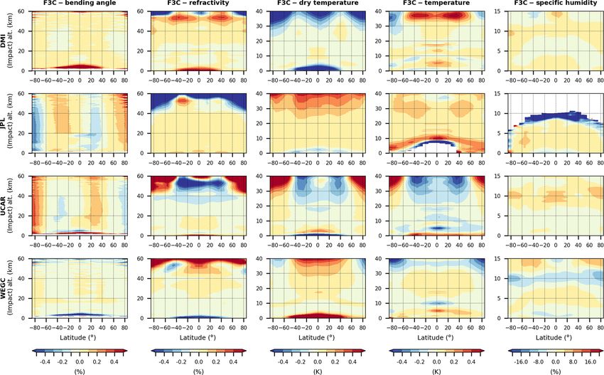
2550                                        A. K. Steiner et al.: Consistency of multi-mission GPS radio occultation records

processed RO data products from bending angle to temper-            2002; Jensen et al., 2003, 2004; Gorbunov et al., 2004;
ature for this study: Danish Meteorological Institute (DMI),        Sokolovskiy et al., 2007). The ionospheric contribution to the
Copenhagen, Denmark; German Research Centre for Geo-                signal is largely removed by differencing the dual-frequency
sciences (GFZ), Potsdam, Germany; Jet Propulsion Labo-              GNSS signals, typically at bending angle level (Vorob’ev and
ratory (JPL), Pasadena, CA, USA; University Corporation             Krasil’nikova, 1994). Current research aims at further min-
for Atmospheric Research (UCAR), Boulder, CO USA; and               imization of the residual ionospheric error (Danzer et al.,
Wegener Center/University of Graz (WEGC), Graz, Aus-                2015). The ionosphere-corrected bending angle represents
tria. Each center has implemented an independently devel-           the cumulative signal refraction due to atmospheric density
oped processing system for the retrieval of RO data products.       gradients.
While the basic steps in the retrieval (Kursinski et al., 1997)        The next retrieval step is the computation of refractivity
are essentially the same, different implementation options are      from bending angle by an Abel transform (Fjeldbo et al.,
chosen by the centers for specific processing steps.                1971). This involves an integral with an upper bound of in-
                                                                    finity. Also, the signal-to-noise ratio of the bending angle de-
2.2    General RO data processing description                       creases with increasing altitude (above about 50 km depend-
                                                                    ing on the thermal noise of the receiver). Therefore, an ini-
Here, we briefly describe the basic retrieval steps from            tialization of bending angle profiles with background infor-
the phase measurements to atmospheric variables for dry             mation is performed at high altitudes. The optimized bending
and moist atmospheric conditions. Table 1 gives a concise           angle profiles are then converted to refractivity profiles.
overview of the retrieval steps and the implementation at              Refractivity at microwave wavelengths in the neutral at-
each center.                                                        mosphere mainly depends on the thermodynamic conditions
   The fundamental measurement is the GNSS signal phase             of the dry and the moist atmosphere and is given by the
change as a function of time, which varies according to the         Smith–Weintraub formula (Smith and Weintraub, 1953) or
optical path length between the transmitter satellite and the       updated formulations (Aparicio and Laroche, 2011; Healy,
LEO receiver satellite. Highly accurate atomic clocks are           2011; Cucurull et al., 2013). Dry density profiles are cal-
the heart of the system, ensuring long-term frequency stabil-       culated from atmospheric refractivity by neglecting the wet
ity. Two coherent carrier signals are transmitted, in the case      term in the formula. Dry pressure profiles are retrieved using
of the US Global Positioning System (GPS) at wavelengths            the hydrostatic equation and dry temperature profiles using
of 0.19 m (L1 signal) and 0.24 m (L2 signal) (Hofmann-              the equation of state for dry air conditions in the upper tro-
Wellenhof et al., 2008; Teunissen and Montenbruck, 2017),           posphere and lower stratosphere. In the lower to middle tro-
which enables removing contributions due to Earth’s iono-           posphere, the retrieval of (physical) atmospheric temperature
sphere in a later retrieval step.                                   or humidity requires additional background information in
   In the retrieval, the Doppler shift, i.e., the time derivative   order to resolve the wet–dry ambiguity information inherent
of the phase, is propagated further (e.g., Melbourne et al.,        in refractivity (e.g., Kursinski et al., 1996; Healy and Eyre,
1994; Kursinski et al., 1997). The kinematic contribution to        2000; Kursinski and Gebhard, 2014). Different methods are
the Doppler shift due to the relative motion of the GNSS            applied for moist air retrievals, including a priori knowledge
and LEO satellites is determined from precise position and          of the state of the atmosphere. Finally, quality control (QC)
velocity information, i.e., precise orbit determination (POD)       is implemented at several processing steps.
(Bertiger et al., 1994; König et al., 2006). Removing it yields        Atmospheric profiles are provided as a function of mean
the Doppler shift due to the Earth’s refractivity field. Errors     sea level (m.s.l.) altitude due to accurate knowledge of trans-
in the receiver clock are removed by single differencing with       mitter and receiver positions (and the assumption of local
a second reference satellite link or with double differencing       spherical symmetry), referred to a reference coordinate sys-
by using additional ground clock information (Wickert et al.,       tem and the Earth’s geoid (see Table 1). The vertical inte-
2002). No differencing is needed, i.e., zero differencing, if       gration of density also provides pressure as a function of
there are ultra-stable clocks aboard the LEO satellites and         altitude. Geopotential height can be computed without the
clock errors are very small, such as for GRACE or Metop             need for information on surface pressure or any other infor-
(e.g., Wickert et al., 2002; Schreiner et al., 2010, 2011; Bai      mation except gravity potential. Further details on vertical
et al., 2018). Geodetic processing systems are used to esti-        coordinates and the geolocation of RO are given in Scherllin-
mate errors in the GNSS transmitter clocks.                         Pirscher et al. (2017).
   For microwave refraction, geometric optics retrieval is
applied to convert Doppler shift to bending angle profiles,         2.3   Center-specific RO processing steps and
assuming local spherical symmetry of the atmosphere. In                   comparison
the lower troposphere, multipath and diffraction effects be-
come important due to atmospheric humidity. Here, wave              Table 1 provides an overview of current state-of-the-art re-
optics methods are applied for the retrieval of bending an-         trieval versions and the processing steps implemented at each
gle using phase and amplitude information (e.g., Gorbunov,          center as well as information on data description and avail-

Atmos. Meas. Tech., 13, 2547–2575, 2020                                              https://doi.org/10.5194/amt-13-2547-2020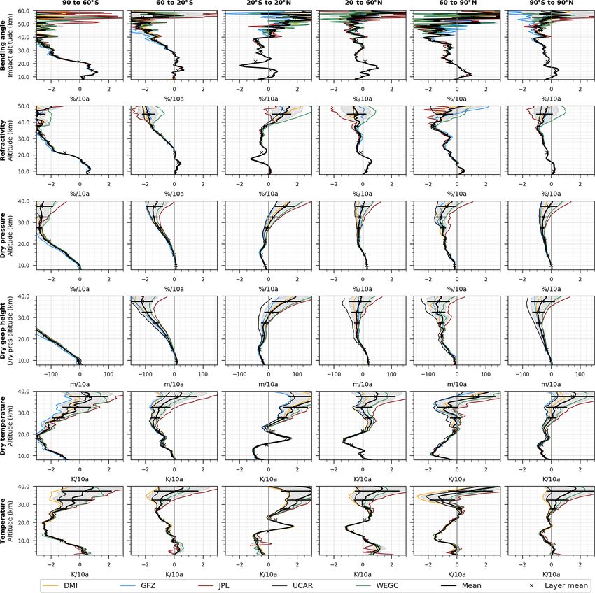
A. K. Steiner et al.: Consistency of multi-mission GPS radio occultation records                                                   2551

Table 1. Overview of processing steps for RO dry and moist air retrieval at DMI, GFZ, JPL, UCAR, and WEGC.

   Processing step       Center   Implementations of each center
   URL                   DMI      http://www.romsaf.org (last access: 14 May 2020)
                         GFZ      http://www.gfz-potsdam.de/en/section/space-geodetic-techniques/topics/gnss-radio-occultation/
                                  (last access: 14 May 2020)
                         JPL      https://genesis.jpl.nasa.gov/genesis/ (last access: 14 May 2020)
                         UCAR     http://cdaac-www.cosmic.ucar.edu (last access: 14 May 2020)
                         WEGC     http://www.wegcenter.at (last access: 14 May 2020)
   Processing version;   DMI      GPAC-2.3.0/ROPP software; orbit as well as excess phase and amplitude data from UCAR
   POD orbit             GFZ      Version POCS ATM version 006; GPS and LEO POD: EPOS-OC, RSO orbit products
   data version                   (König et al., 2006); excess phase: CHAMP, single differencing,
   and phase                      reference link smoothing; GRACE: zero differencing
                         JPL      Version 2.7 processing (single differencing, cubic phase smoothing); POD: GPS orbits from
                                  JPL FLINN products; LEOs with reduced dynamic strategy
                                  using GIPSY software (Bertiger et al., 1994)
                         UCAR     CDAAC version 4.6; GPS final-orbit products from CODE (for CHAMP, METOP) and
                                  IGS (for COSMIC), LEO reduced-dynamic orbits using Bernese v5.2
                         WEGC     OPSv5.6; UCAR/CDAAC orbit, phase, and amplitude data (Angerer et al., 2017; Table 1)
   Calculation of        DMI      Canonical transform (CT2) inversion < 20 km (Gorbunov and Lauritsen, 2004), transition to
   bending angle                  geometric optics (GO) inversion at 20–25 km, GO > 25 km
   (BA)                  GFZ      Full spectrum inversion (FSI) < 15 km (Jensen et al., 2003), smooth transition between
                                  11 and 15 km to GO, GO > 15 km
                         JPL      Canonical transform (CT) after Gorbunov (2002) applied to L1 at impact height < 30 km;
                                  GO for L1 > 30 km and L2 at all heights
                         UCAR     Phase matching < 20 km (Jensen et al., 2004), GO > 20 km
                         WEGC     CT2 inversion (Gorbunov and Lauritsen, 2004) with a Gaussian transition of 4.5 km width
                                  and variable center height between 7 and 13 km, GO above
   Ionospheric           All      Linear combination of L1 and L2 BA (Vorob’ev and Krasil’nikova, 1994)
   correction            DMI      Linear combination, ionospheric correction extrapolated with constant L1–L2 BA below
                                  dynamic L2 height – transition over 2 km
                         GFZ      Linear combination, ionospheric correction extrapolated with constant L1–L2
                                  BA below 12 km
                         JPL      Linear combination, ionospheric corr. term extrapolation < 10 km when L2 1 s SNR < 30 V/V
                         UCAR     Above 20 km: correction of L1 BA by L1–L2 BA smoothed with window determined
                                  individually for each occultation to minimize combined noise (Sokolovskiy et al., 2009);
                                  below 20 km: L1 BA corrected by a three-parameter function fitted to observational
                                  L1–L2 BA at 20–80 km (Zeng et al., 2016)
                         WEGC     Linear combination, ionospheric correction term extrapolated with linear L1–L2 BA < 15 km
   Initialization        DMI      Optimization with dynamic estimation of observation errors (Gorbunov, 2002) and background
   of BA                          errors fixed at 50 %, background based on BAROCLIM (best
                                  global fit to data between 40 and 60 km, scaled using two-parameter
                                  regression) (Scherllin-Pirscher et al., 2015)
                         GFZ      Optimization after Sokolovskiy and Hunt (1996) with MSISE-90 (> 40 km), observation error
                                  variance estimated as 25 % of mean observation–background
                                  deviation between 60 and 70 km
                         JPL      Exponential function fit at 50–60 km and extrapolation > 60 km impact height
                         UCAR     Static optimization (independent of the observational noise), two-parameter fitting of NCAR BA
                                  climatology (Randel et al., 2002) to observational BA in 35–60 km interval, transition to fitted
                                  BA climatology in the same interval, transition to unfitted BA climatology in the 55–65 km interval
                         WEGC     Optimization > 30 km with ECMWF short-range forecasts (24 or 30 h) and above with MSISE-90
                                  to 120 km, dynamic estimation of observation errors and inverse covariance weighting
                                  (Schwärz et al., 2016; Appendix A.4)

https://doi.org/10.5194/amt-13-2547-2020                                                Atmos. Meas. Tech., 13, 2547–2575, 2020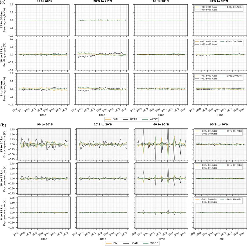
2552                                        A. K. Steiner et al.: Consistency of multi-mission GPS radio occultation records

Table 1. Continued.

  Processing step          Center   Implementations of each center
  Refractivity retrieval   All      Abel inversion (Fjeldbo et al., 1971) of optimized bending angle profile
                           DMI      Abel inversion below 150 km
                           GFZ      Abel Inversion below 150 km
                           JPL      Abel Inversion below 120 km
                           UCAR     Abel inversion below 150 km
                           WEGC     Abel inversion below 120 km
  Dry air retrieval        All      Refractivity (N) is directly proportional to air density (ideal gas equation)
                           DMI      Pressure integration, hydrostatic integral initialization at 150 km, upper boundary condition
                                    from refractivity gradient, geopotential height relative to EGM-96 geoid
                           GFZ      Hydrostatic integral initialization at 100 km with MSISE-90 pressure,
                                    geopotential height relative to EGM-96
                           JPL      Hydrostatic integral initialization at 40 km using ECMWF analysis,
                                    geopotential height relative to JGM-3
                           UCAR     Hydrostatic integral initialization at 150 km with zero boundary condition
                           WEGC     Hydrostatic integral initialization at 120 km with MSISE-90 pressure,
                                    geopotential height relative to EGM-96
                           All      Dry temperature (Td ) is obtained using the Smith–Weintraub formula for dry air
                                    (Smith and Weintraub, 1953) and the equation of state (ideal gas)
  Moist air retrieval      DMI      1D-Var using ERA-Interim as background and refractivity observations as input
                           GFZ      Not included, but relevant data products can be provided on demand
                           JPL      Direct method using temperature and specific humidity from ECMWF analysis when T > 250 K
                                    (Kursinski et al., 1996)
                           UCAR     1D-Var using ERA-Interim as background and refractivity observations (Wee, 2005)
                           WEGC     Above 16 km: calculation of physical temperature T and pressure p using a first-order
                                    approximation for the ratio between p and dry pressure pd .
                                    Below 14 km: with half-sine transition between 16 and 14 km, simplified 1D-Var.
                                    – retrieval of T and p using ECMWF short-range forecast specific humidity qB
                                    – retrieval of q and p using ECMWF short-range forecast temperature TB
                                    – statistical optimization of T and q with TB and qB , background standard errors from ROPPv6.0
                                    (Culverwell and Healy, 2011), RO observational standard error (Scherllin-Pirscher et al., 2011a)
  Quality control (QC)     DMI      Provider QC (reject if phase data are flagged);
                                    QC of L2 quality from impact parameters (reject if noise is too large);
                                    QC of BA using ERA-Interim forecasts (reject if > 90 % in 10–40 km);
                                    QC of regression parameters (reject if too far from 1.0);
                                    QC of optimized BA using background (reject if > 5 µrad above 60 km);
                                    QC of background weight in optimization (reject if > 10% below 40 km);
                                    QC of refractivity using ERA-Interim forecasts (reject if > 10 % in 10–35 km);
                                    QC of dry temperature using ERA-Interim forecasts (reject if > 20 K in 30–40 km);
                                    QC of 1D-Var cost function (reject if too large) and convergence (reject if too many iterations)
                           GFZ      Minimum duration of occultation event: 20 s
                                    Quotient L1/L2 excess phase forward differences between 0.97 and 1.03 for at least 650 connected
                                    data samples; QC of refractivity N using MSISE-90: reject if 1N > 22.5 % between 8 and 31 km
                           JPL      Refractivity difference with ECMWF < 10 % between 0 and 40 km and temperature difference with
                                    ECMWF < 10 K below 40 km
                           UCAR     Multiple QC checks including the following.
                                    – Comparison of retrieved N and N from NCAR climatology (Randel et al., 2002);
                                    – Comparison of maximum relative BA difference between RO and NCAR climatology;
                                    – BA error check of local spectral width;
                                    – SNR too low;
                                    – Check of L2 data quality by comparison of maximum L1–L2 Doppler;
                                    – Checks of mean and standard deviation of difference in retrieved and climatological BA
                                    between 60 and 80 km

Atmos. Meas. Tech., 13, 2547–2575, 2020                                                   https://doi.org/10.5194/amt-13-2547-2020
A. K. Steiner et al.: Consistency of multi-mission GPS radio occultation records                                                             2553

Table 1. Continued.

    Processing step    Center    Implementations of each center
                       WEGC      Raw QC check: straight line tangent point altitude (SLTA) range at least between 65 and 20 km;
                                 GO only QC of BA:
                                 – cut off < 15 km impact height if gradient is too large;
                                 – reject if BA < 0 rad below 50 km;
                                 – reject if bias relative to MSIS-90 > 10−5 rad;
                                 – reject if standard deviation relative to MSIS-90 > 5 × 10⁻⁵ rad
                                 WO only QC: cut off data at bottom of measurement if
                                 – amplitude of CA signal is lower than 10 % of max amplitude;
                                 – smoothed GO BA (over 3 km) exceeds 0.05 rad;
                                 – smoothed impact parameter (over 3 km) < 0 m;
                                 – SLTA < −250 km
                                 QC of BA, N, T using ECMWF analyses: reject if
                                 1BA > 20 %, 1N > 10 % in 5–35 km, or 1T > 20 K in 8–25 km (Angerer et al., 2017)
    Reference frame    DMI       Earth figure: WGS-84 ellipsoid; vertical coordinate: mean sea level (m.s.l.) altitude;
    vertical                     conversion of ellipsoidal height to m.s.l. altitude (at SLTA = 0 TP location) via EGM-96 geoid
    coordinate                   smoothed to 1◦ × 1◦ resolution
                       GFZ       Earth figure: WGS-84 ellipsoid, EGM-96 geoid used for altitude above m.s.l. calculation
                       JPL       Earth figure: IERS Standards 1989 ellipsoid; vertical coordinate: m.s.l. altitude computed
                                 using the JGM3/OSU91A geoid truncation at spherical harmonic degree 36
                       UCAR      Earth figure: WGS-84 ellipsoid; the occultation point is determined using BA for CIRA+Q climatology
                                 (Kirchengast et al., 1999) and 500 m observed excess phase; the center of the reference frame is in the
                                 local center of curvature of the reference ellipsoid at the occultation point (Syndergaard, 1998)
                                 in the direction of the occultation plane; JGM2 geoid undulation is used to calculate m.s.l. altitude
                       WEGC      Earth figure: WGS-84 ellipsoid; vertical coordinate: m.s.l. altitude; conversion of ellipsoidal height to
                                 m.s.l. altitude (at SLTA = 0 TP location) via EGM96 smoothed to 2◦ × 2◦ resolution
                       All       Bending angle is given as a function of impact altitude, i.e., impact parameter minus radius of curvature
                                 minus the undulation of the geoid; the impact parameter is defined as the perpendicular distance
                                 between the local center of curvature and the ray path from the GPS satellite
    Reference and/     DMI       ROM SAF ATBD documents: http://www.romsaf.org/product_archive.php (last access: 14 May 2020)
    or publication     GFZ       ftp://isdcftp.gfz-potsdam.de/ (last access: 14 May 2020)
                       JPL       Hajj et al. (2002)
                       UCAR      CDAAC website documentation area:
                                 http://cdaac-www.cosmic.ucar.edu/cdaac/doc/overview.html (last access: 14 May 2020)
                       WEGC      https://doi.org/10.25364/WEGC/OPS5.6:2019.1; Schwärz et al. (2016), Angerer et al. (2017)

ability (Steiner et al., 2013; Table 1 updated for current pro-          a background bending angle. Each center uses different back-
cessing versions and extended for moist air processing steps).           ground information: atmosphere model climatologies (GFZ,
Three of the RO centers (GFZ, JPL, UCAR) have the full pro-              UCAR), observation-based climatologies (DMI), or short-
cessing chain implemented, going from the raw data level to              range forecasts (WEGC). Handling of observational and
atmospheric variables. Two centers (DMI and WEGC) start                  background errors affects the amount of information from
their processing at the phase data level in this study by using          observations and from the background included in the re-
phase data and orbit data from UCAR/CDAAC (COSMIC                        trieved optimized bending angle. Observational error is typ-
Data Analysis and Archive Center). Thus, as some centers                 ically smaller in data from RO systems with improved per-
start with the same phase and orbit data (from UCAR), the                formance, i.e., lower thermal noise or higher-gain antennas
products from raw data to atmospheric parameters are not                 enabling a higher signal-to-noise ratio up to higher altitudes.
strictly independent for these centers.                                  In the different moist air retrieval implementations, a priori
   The main differences between the centers’ processing                  information is also included, stemming either from atmo-
steps include the initialization of the Abel integral that trans-        spheric analyses or forecasts (JPL, WEGC), model forecasts
forms bending angles to refractivity, moist air retrieval, and           produced with reanalysis (DMI), or reanalyses (UCAR).
quality control. For the bending angle vertical profiles, JPL               Figure 1 shows the number of profiles per month deliv-
performs an extrapolation of the bending angle to higher al-             ered by each center for each RO mission. Also indicated is
titudes, while the other centers apply statistical optimization          the number of profiles in the common subsets, which we
methods that combine the bending angle measurements with                 used in the profile-to-profile intercomparison for quantify-

https://doi.org/10.5194/amt-13-2547-2020                                                     Atmos. Meas. Tech., 13, 2547–2575, 2020
2554                                      A. K. Steiner et al.: Consistency of multi-mission GPS radio occultation records

Figure 1. Number of RO profiles per month delivered by each processing center, DMI (yellow), GFZ (blue), JPL (red), UCAR (black),
and WEGC (green), and the maximum subset of profiles (gray), shown for the respective time periods of the four missions CHAMP, F3C,
GRACE, and Metop.

ing structural uncertainty. For CHAMP, GFZ delivered the            3   Study setup and analysis method
largest number of data, followed by UCAR, DMI, WEGC,
and JPL. There is a data gap in July 2006 when CHAMP had
very few measurements. The common subset of profiles for            We investigated the structural uncertainty of the following
CHAMP summed up on average to about 1500 profiles per               RO variables: bending angle (α), optimized bending angle
month.                                                              (αopt ), refractivity (N ), dry pressure (pdry ), dry temperature
   For F3C, DMI, UCAR, and WEGC delivered nearly the                (Tdry ), dry geopotential height (Zdry ), pressure (p), temper-
same number of data, and only JPL provided a smaller                ature (T ), and specific humidity (q). The atmospheric pro-
amount. GFZ did not process F3C data. The number of F3C             files were provided on a 100 m m.s.l. altitude grid except
measurements was highest from 2007 to 2010, with more               bending angle, which was given on impact altitude, and
than 70 000 profiles per month, and decreased over time             geopotential height, which was related to dry pressure levels,
as the satellites successively ceased achieving full function.      i.e., “dry pressure altitude” defined as zp (m) = (7000 m)·
The mission design life was 2 years. Only two of the six            ln(1013.25 hPa / pdry ; hPa).
F3C satellites still produced data in 2018. For this study,            Table 2 summarizes the data delivered for this study by
UCAR provided a reprocessed F3C data set until April 2014.          each center and gives information on satellite missions, time
The common subset of F3C data ranged from 20 000 up to              periods, and atmospheric variables. Not all of the centers pro-
50 000 profiles per month over time.                                vided data for each satellite and each variable. UCAR did not
   Data for GRACE were provided by three centers, DMI,              provide optimized bending angle profiles. GFZ did not pro-
GFZ, WEGC, delivering nearly the same number of profiles            vide moist air variables. This was adequately considered in
with a common subset of about 3000 profiles per month.              the computations.
Metop data were provided by DMI, UCAR, and WEGC,                       The study was based on the intercomparison of collocated
with a common subset of about 15 000 profiles increasing            profiles between the centers for each satellite mission and
to 25 000 per month when the second Metop satellite started         atmospheric variable. The profiles were collocated based on
measuring.                                                          a unique event identifier (ID) including information on re-
   The number of common profiles is noticeably smaller than         ceiver ID, GPS satellite ID, date, and time of the observa-
the number of profiles delivered by any of the centers, which       tion. The common subset of data was analyzed further. This
is mainly due to the different quality control handling. This       means that only the common time periods can be intercom-
means that each center does not deliver the same set of pro-        pared for which each center provided data continuously. The
files.                                                              investigated periods are September 2001–September 2008
                                                                    for CHAMP (five centers), March 2007–December 2016 for
                                                                    GRACE (three centers), August 2006–April 2014 for F3C
                                                                    (four centers), and March 2008–December 2015 for Metop
                                                                    (three centers).

Atmos. Meas. Tech., 13, 2547–2575, 2020                                              https://doi.org/10.5194/amt-13-2547-2020
A. K. Steiner et al.: Consistency of multi-mission GPS radio occultation records                                                                        2555

Table 2. Overview of RO data delivered by the different processing centers and the common time periods used in this study: processing
center, satellite mission, time period, and variables.

                                Center                      Satellites         Period                Variables
                                All centers’                CHAMP              09/2001–09/2008
                                common periods              COSMIC             08/2006–04/2014
                                (used in this study)        GRACE              03/2007–12/2016
                                                            METOP              03/2008–12/2015
                                DMI                         CHAMP              09/2001–09/2008       All variables∗
                                                            COSMIC             05/2006–12/2016       All variables
                                                            GRACE              03/2007–12/2016       All variables
                                                            METOP              02/2008–12/2016       All variables
                                GFZ                         CHAMP              05/2001–09/2008       All except: p, T , q
                                                            GRACE              02/2006–11/2017       All except: p, T , q
                                JPL                         CHAMP              04/2001–09/2008       All variables
                                                            COSMIC             05/2006–12/2016       All variables
                                UCAR                        CHAMP              05/2001–09/2008       All except: αopt
                                                            COSMIC             05/2006–04/2014       All except: αopt
                                                            METOP              02/2008–12/2015       All except: αopt
                                WEGC                        CHAMP              05/2001–09/2008       All variables
                                                            COSMIC             08/2006–12/2018       All variables
                                                            GRACE              03/2007–11/2017       All variables
                                                            METOP              02/2008–12/2018       All variables
                              ∗ All variables include α , α , N , p , T , Z , p , T , and q .
                                                           opt     dry dry dry

   We first calculated the differences (1Xi ) of each center (c)                      We performed the calculations for each atmospheric pa-
to the all-center mean (i.e., mean of all centers) (Xiall ) over                   rameter (X) for each satellite mission (s) of each center (c)
time based on individual profiles of atmospheric parameters                        given at monthly resolution (t) for latitude bands (φ) and al-
(Xi ), with i denoting the index of matched profiles and ncenter                   titude levels (z), i.e., nine parameters, four satellite missions,
denoting the number of centers, using Eqs. (1) and (2):                            and five centers, for 18 latitude bands and up to 600 altitude
                                                                                   levels as well as for six large latitude bands and up to eight
          1   Xncenter                                                             altitude layers (after Steiner et al., 2013; Mochart, 2018).
Xiall =          c=1
                         Xi (c) ,                                        (1)          The mean difference of each center to the all-center mean
     ncenter
             all
                                                                                   was computed by averaging over the satellite-dependent pe-
1Xi = Xi − Xi .                                                          (2)       riod, with ntime as the number of time steps (months), using
                                                                                   Eq. (3):
The profiles (Xi , 1Xi , Xiall ) were then binned into 10◦ zonal                                                1 Xntime
bands and averaged to monthly medians (X, 1X, Xall ). By

                                                                                   1X ci , φj , zk , sm =               l=1
                                                                                                                               1X ci , φj , zk , tl , sm . (3)
                                                                                                             ntime
using difference time series we remove the climate variabil-
ity that is common in the data sets. Anomaly difference time                       Results from these computations are discussed in Sect. 4.1.
series were then computed by subtracting the mean annual                              The annual cycle for the differences to the all-center mean
cycle for the respective time period (see Table 2) to reduce                       was computed using Eq. (4). The number of years over which
the natural variability in the differences. Percentage anomaly                     the annual cycle was calculated is denoted nyr , the index l 0
difference time series were computed for variables that de-                        takes the values 1 to 12, and τl 0 denotes one of the 12 months
crease exponentially with altitude.                                                of a year:
   The spread of the anomaly difference trends and the spread
of the center trends were used for estimating the structural
                                                                                                                            1 Xnyr
                                                                                   1X AnnCycle ci , φj , zk , τl 0 , sm =             l 00 =1
uncertainty (Wigley, 2006) of RO records. For each atmo-                                                                  nyr
spheric variable and satellite mission, we computed the lin-

                                                                                              1X ci , φj , zk , tl 0 +12·(l 00 −1) , sm .                 (4)
ear trend over the respective time period for the all-center
mean and for each center. The standard deviation of the cen-                       Subtracting the annual cycle provided the de-seasonalized
ter trends was finally used as a measure of the spread.                            anomaly differences for each center c and satellite mission

https://doi.org/10.5194/amt-13-2547-2020                                                                 Atmos. Meas. Tech., 13, 2547–2575, 2020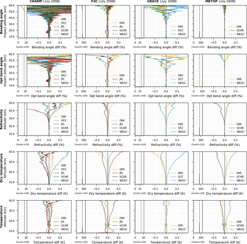
2556                                            A. K. Steiner et al.: Consistency of multi-mission GPS radio occultation records

s, obtained according to Eq. (5):                                         ber of data available. For CHAMP, the bending angle be-
                                                                        comes noisy near 35–40 and above 40–50 km for the other
1XDeseasAnomDiff ci , φj , zk , tl , sm = 1X ci , φj , zk , tl , sm       RO missions. The optimization of the bending angle reduces

  − 1X AnnCycle ci , φj , zk , τ1+(l−1) mod 12 , sm .               (5)   the noise and stabilizes the retrieval at high altitudes above
                                                                          50 km. The noise reduction is visible in the optimized bend-
Fractional (percentage) de-seasonalized anomaly differences               ing angle differences, specifically for F3C, GRACE, and
were computed analogously.                                                Metop. The bending angle differences are < 0.1 % from a 10–
   Linear trends were then computed with standard linear re-              40 to 50 km impact altitude, depending on the mission.
gression for the de-seasonalized anomaly difference time se-                 In the RO retrieval chain of further derived parameters,
ries and, analogously, for the de-seasonalized time series of             such as refractivity, pressure, or dry temperature, the impact
each center. Results from these computations are discussed                of background information propagates further downward in
in Sect. 4.2 and 4.3. For better comparison, the trends are               altitude for each retrieved parameter. Refractivity, which is
stated per 10 years. However, we do not discuss climato-                  proportional to atmospheric density, shows differences of
logical trends here as the time periods are different for each            < 0.05 % at 10–30 km for all satellites in July 2008. Dry tem-
RO mission. We are interested in the structural uncertainty               perature differences are small from 8–25 to 30 km depending
of trends represented by the standard deviation of the ncenter            on the mission. Physical temperatures, usually derived with a
individual center trends. This measure gives us an indication             priori information, show similar differences, with JPL show-
of the stability of the multi-satellite RO records.                       ing larger deviations due to cutoff artifacts below 15 km (see
   We performed the computations for 10◦ zonal medians,                   below).
averaging the collocated individual RO profiles on the given                 Next, we give an overview of mean differences with re-
vertical grid on a monthly median basis. We then averaged                 spect to the all-center mean, averaged over the full time
to larger latitudinal domains and altitude layers, in which               period of a mission, which we exemplarily show for the
RO data show similar behavior and similar structural un-                  F3C mission. Figure 3 presents averaged anomaly differ-
certainty. We defined six latitude bands: the tropics (TRO;               ences for bending angle, refractivity, dry temperature, tem-
20◦ N–20◦ S), northern and southern midlatitudes (NML and                 perature, and specific humidity for 10◦ zonal means at a
SML; 20–60◦ N and 20–60◦ S), northern and southern high                   100 m vertical grid. The mean differences for bending an-
latitudes (NHL and SHL; 60–90◦ N and 60–90◦ S), and a                     gle are found to be very small (0.1 %–0.2 %) at all lati-
global band (GLOB; 90◦ N–90◦ S). We defined (up to) eight                 tudes, except at high latitudes where differences are larger
altitude layers. The uppermost altitude levels are 60 km for              for JPL and UCAR bending angles. Different choices for the
bending angle, 50 km for refractivity, and 40 km for the other            bending angle initialization by the centers are reflected in
variables except humidity (15 km). The inspected vertical                 larger refractivity differences above about 40 km, while be-
layers include 8–18, 18–25, 25–30, 30–35, 35–40, 40–50,                   low the mean differences are very small (< 0.1 %). For subse-
and 50–60 km. Structural uncertainty in trends is finally pre-            quent derived variables, the differences become larger above
sented at the full 100 m altitude grid.                                   30 km as seen for dry temperature. There, some latitude-
                                                                          dependent features appear that might stem from high-altitude
4     Results and discussion                                              initialization in the retrieval, specifically at high latitudes.
                                                                          At 5–30 km, mean differences for dry temperature are found
4.1    Comparison of differences in multi-satellite RO                    to be < 0.2 K for all latitude bands. Physical temperature
       profiles for one exemplary month and for the total                 shows similar differences of < 0.2 K at 2–30 km of altitude.
       mean                                                               JPL provides physical temperature products only down to
                                                                          a certain altitude. RO temperature is cut off when it rises
As a first overview, we present comparison results for one                above 240 K in their moist air retrieval, for which back-
exemplary month, July 2008, for selected atmospheric RO                   ground temperature information from ECMWF (European
variables in order to introduce several characteristic features.          Centre for Medium-Range Weather Forecasts) analyses is
Figure 2 shows the global mean difference of profiles from                used to derive specific humidity. DMI and UCAR use a one-
each center with respect to the all-center mean for the mis-              dimensional variational (1D-Var) method to derive tempera-
sions CHAMP, F3C, GRACE, and Metop. Differences for the                   ture with ERA-Interim (ECMWF Reanalysis-Interim) prod-
variables bending angle, optimized bending angle, refractiv-              ucts as background. WEGC applies a simplified 1D-Var re-
ity, dry temperature, and physical temperature are presented.             trieval method using ECMWF forecasts as background be-
Note that deviations of one center are counterbalanced by                 low about 16 km of altitude. Above this altitude, WEGC dry
other centers due to referencing to the all-center mean.                  and physical temperatures are the same. However, in Fig. 3,
   The mean difference profiles for non-optimized bending                 differences are shown with respect to the all-center mean,
angle and bending angle are smaller at upper altitudes for                and the latter is different for dry and physical temperature.
F3C, GRACE, and Metop compared to CHAMP due to en-                        For specific humidity we find mean differences of each cen-
hanced receiver quality and smoother due to the larger num-               ter to the all-center mean of < 15 %. JPL provides specific hu-

Atmos. Meas. Tech., 13, 2547–2575, 2020                                                    https://doi.org/10.5194/amt-13-2547-2020
A. K. Steiner et al.: Consistency of multi-mission GPS radio occultation records 2557 Figure 2. Global mean difference of atmospheric profiles from each center to the all-center mean for one exemplary month (July 2008) based on 10◦ zonal medians and shown for the satellite missions CHAMP, F3C, GRACE, and Metop (left to right) for bending angle, optimized bending angle, refractivity, dry temperature, and temperature (top to bottom). The number of data points is shown in the left sub-panels. midity data up to 10 km of altitude only in synergy with the Comparison of mean differences with data from the other temperature cutoff, and the number of data decreases above satellite missions CHAMP, GRACE, and Metop shows good 8 km. The larger differences at this altitude are artifacts and consistency over the same regions; however, differences can be removed with a more rigid cutoff. Only a few centers are found to be smaller at higher altitudes, specifically for delivered humidity and the data have different height avail- Metop. Commonalities and differences are further investi- ability, which hampers a rigorous statistical intercomparison gated in the full difference time series and revealed in the of humidity in this study. We thus do not show further com- structural uncertainty estimates. parisons here. https://doi.org/10.5194/amt-13-2547-2020 Atmos. Meas. Tech., 13, 2547–2575, 2020
2558 A. K. Steiner et al.: Consistency of multi-mission GPS radio occultation records
Figure 3. Mean difference of each center, DMI, JPL, UCAR, and WEGC (top to bottom), to the all-center mean for F3C data averaged over
August 2006–April 2014 based on 10◦ zonal medians and shown for bending angle, refractivity, dry temperature, temperature, and specific
humidity (left to right).
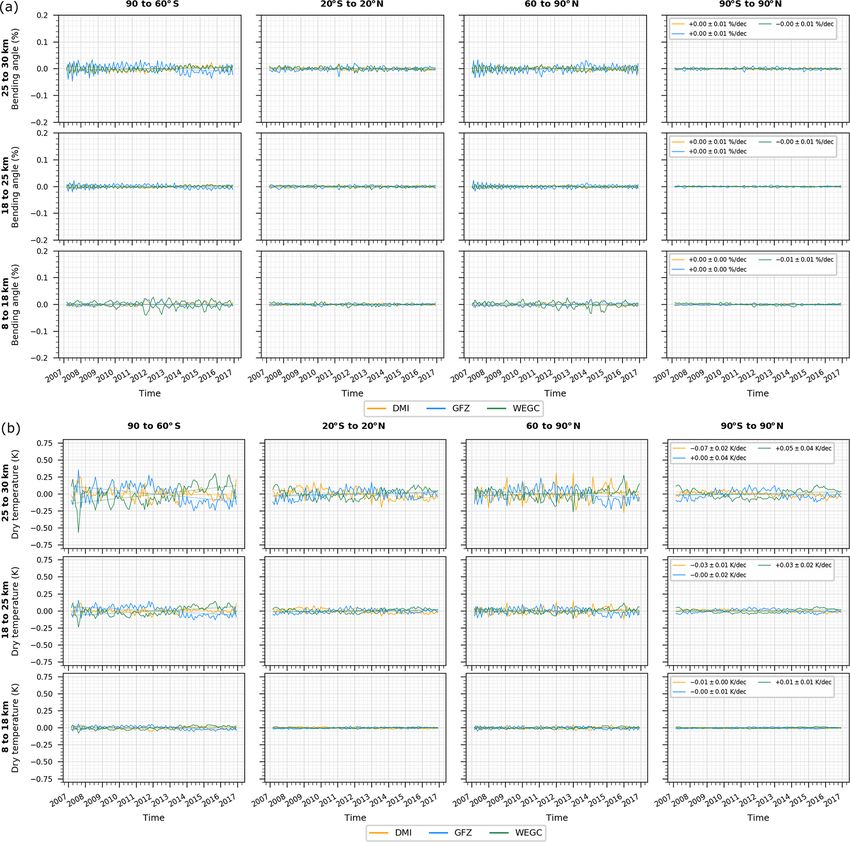
4.2 Comparison of anomaly difference time series about ±0.05 % per decade below 25 km, increasing to about
±0.1 % per decade above. At SHL, a larger difference trend
is seen for GFZ at 25–30 km. Larger variability in bending
Here, we investigate anomaly difference time series (see angle is found for JPL over the investigated period. The dif-
Eq. 5) for each satellite mission (CHAMP, F3C, GRACE, ference time series in CHAMP bending angle show similar
Metop) over the respective time periods as presented in behavior at high latitudes and in the tropics. The global mean
Figs. 4 to 7. We show monthly median differences to the difference trends (90◦ S–90◦ N) for CHAMP are ±0.04 % per
all-center mean for two selected variables, bending angle decade at 8–18 km and ±0.02 % per decade above.
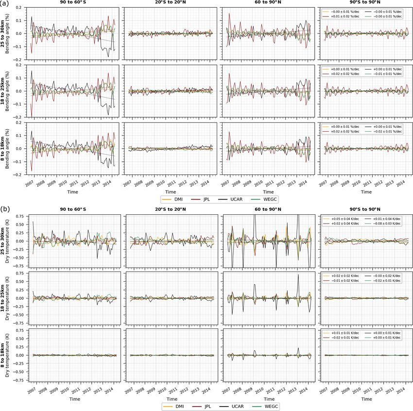
and dry temperature. Bending angle is at the beginning of For F3C, the spread of mean anomaly difference trends
the processing chain (after phase data processing), while dry (Fig. 5a) is found to be larger at high latitudes than in the
temperature is one of the final RO products commonly used tropics. The largest difference trends are found at SHL, with
in climate studies. We present results for the global mean a spread of −0.17 % to 0.1 % per decade in all altitude layers.
(GLO) and for selected zonal means, the tropics (TRO), and This is due to a small shift in UCAR bending angle in 2013,
high latitudes (SHL, NHL). We do not show results for the which is currently under investigation. In the tropics, the dif-
midlatitude bands (NML, SML) as the results are similar to ferences are small. In the global mean, the spread in differ-
those in the tropics. We investigate consistencies and devia- ence trends is ±0.02 % per decade at 18–25 km and ±0.01 %
tions in the anomaly difference time series of individual cen- per decade at 25–30 km, which is smaller than for CHAMP.
ters from the all-center mean. GRACE shows highly consistent anomaly differences
For all satellite missions we find that bending angle dif- (Fig. 6a) and similar behavior at all latitudes. An interest-
ferences are overall very small and consistent below 30 km ing feature in GFZ bending angle is an oscillating variability
at all latitudes. However, there are some differences that over time for GRACE data. However, the spread in differ-
we discuss in the following. For CHAMP, the spread of ence trends is very small at ±0.01 % in all altitude layers.
mean anomaly difference trends in bending angle (Fig. 4a) is Globally it is zero. Also, for Metop we find high consistency
larger than for the other missions. For the zonal means, it is
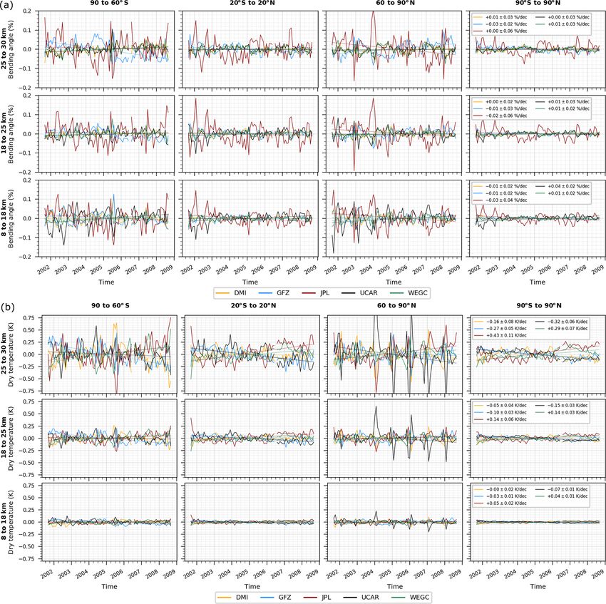
Atmos. Meas. Tech., 13, 2547–2575, 2020 https://doi.org/10.5194/amt-13-2547-2020A. K. Steiner et al.: Consistency of multi-mission GPS radio occultation records 2559 Figure 4. CHAMP bending angle (a) and dry temperature (b) de-seasonalized anomaly difference time series based on 10◦ zonal medians of each center to the all-center mean for latitude bands 90 to 60◦ S, 20◦ S to 20◦ N, 60 to 90◦ N, and globally 90◦ S to 90◦ N (left to right) for altitude layers 8–18, 18–25, and 25–30 km (bottom to top). Time series from DMI (orange), GFZ (blue), JPL (red), UCAR (black), and WEGC (green) are shown. in anomaly differences (Fig. 7a), with a spread in difference ±0.01 % to ±0.02 % per decade at all latitudes at 8–30 km trends of ±0.02 % per decade for bending angle except in for F3C, GRACE, and Metop and near zero globally. For the tropical band. There, differences are slightly larger at CHAMP, it is within ±0.02 % to ±0.03 % per decade, and ±0.05 % per decade at 18–25 km. larger differences only occur for GFZ time series at high lat- For refractivity, we find high consistency in the difference itudes. trends (not shown here for the time series but shown later For dry temperature, the difference time series show some in Sect. 4.3). The spread of the difference trends is about common features for all satellites. We find that the spread in https://doi.org/10.5194/amt-13-2547-2020 Atmos. Meas. Tech., 13, 2547–2575, 2020
2560                                          A. K. Steiner et al.: Consistency of multi-mission GPS radio occultation records

Figure 5. F3C bending angle (a) and dry temperature (b) de-seasonalized anomaly difference time series based on 10◦ zonal medians of
each center to the all-center mean for latitude bands 90 to 60◦ S, 20◦ S to 20◦ N, 60 to 90◦ N, and globally 90◦ S to 90◦ N (left to right) for
altitude layers 8–18, 18–25, and 25–30 km (bottom to top). Time series from DMI (orange), JPL (red), UCAR (black), and WEGC (green)
are shown.

anomaly difference trends for dry temperature is smallest in                 The global mean difference trends for CHAMP range from
the troposphere layer (8–18 km), larger in the lower strato-              about ±0.06 K per decade at 8–18 km to ±0.15 K per decade
sphere layer (18–25 km), and further increases above. The                 at 18–25 km and to about ±0.4 K per decade at 25–30 km.
spread in difference trends is found to be largest for CHAMP              For F3C, the global spread is only ±0.02 K per decade at
(Fig. 4b), followed by F3C (Fig. 5b), GRACE (Fig. 6b), and                8–25 km to ±0.08 K per decade at 25–30 km. For GRACE,
Metop (Fig. 7b).                                                          it is even smaller at ±0.01 K per decade at lower altitudes,
                                                                          increasing to ±0.06 K per decade at 25–30 km. For Metop,

Atmos. Meas. Tech., 13, 2547–2575, 2020                                                      https://doi.org/10.5194/amt-13-2547-2020
A. K. Steiner et al.: Consistency of multi-mission GPS radio occultation records 2561
Figure 6. GRACE bending angle (a) and dry temperature (b) de-seasonalized anomaly difference time series based on 10◦ zonal medians of
each center to the all-center mean for latitude bands 90 to 60◦ S, 20◦ S to 20◦ N, 60 to 90◦ N, and globally 90◦ S to 90◦ N (left to right) for
altitude layers 8–18, 18–25, and 25–30 km (bottom to top). Time series from DMI (orange), GFZ (blue), and WEGC (green) are shown.
it is near zero in the troposphere, ±0.02 K per decade in the peaks can be explained by high-altitude initialization with the
lower stratosphere, and −0.07 to +0.02 K per decade above. NCAR climatology, which does not capture the extraordinary
For CHAMP dry temperature, some larger differences oc- large temperature changes at high latitudes during sudden
cur in the tropics. There, the JPL time series show a slight stratospheric warmings. For GRACE, a peak in WEGC data
shift, which is most prominent at upper altitude levels. Some is seen at the beginning of the time series at upper height lev-
deviations occur in the UCAR time series for some win- els. However, in the global average, the anomaly differences
ter months at NHL. These peaks are only visible for a few are found to be very small despite some larger deviations
months when sudden stratospheric warmings occurred. The in some NHL winter months. Also, the results for physical
https://doi.org/10.5194/amt-13-2547-2020 Atmos. Meas. Tech., 13, 2547–2575, 2020You can also read