Analysing port and shipping operations using big data - Christopher Bonham, Alex Noyvirt, Ioannis Tsalamanis and Sonia Williams

Analysing port and shipping
 operations using big data

Christopher Bonham, Alex Noyvirt, Ioannis Tsalamanis and Sonia Williams

 Data Science Campus, ONS, Christopher.bonham@ons.gov.uk
 18 June 2018

Executive summary
The maritime freight industry is of critical importance to the economic output of the UK, with almost half a billion
tonnes of freight being handled by UK ports in 2016. The Freight Transportation Association estimate that delays on
both side of the Channel cost the UK logistics industry £750,000 a day1. As the demands upon shipping freight are
likely to increase in the future, a more in-depth understanding of the UK maritime shipping industry becomes
increasingly more important.

This report outlines the work undertaken by the Data Science Campus to explore the operation, use and relationships
between ports in the UK at a macro level and the behaviour and operational characteristics of ships at a micro level,
specifically:
• national and international relationships
• traffic at ports and related factors
• inbound delays
• capacity utilisation

Two sources of data are utilised:
• Automatic Identification System (AIS). AIS data records the position, speed, heading, bearing and rate of turn for
 each ship, at frequent time intervals throughout its voyage
• Consolidated European Reporting System (CERS). CERS data is collected at a higher level and records details such
 as destination port and expected time of arrival for the voyage of each ship

A means of storing, decoding and processing AIS data is proposed. A means by which AIS and CERS data can be merged
is presented, allowing a more comprehensive analysis to be undertaken when compared with exploring each dataset
in isolation. Exploratory analysis of both datasets uncovers several insights for ships using the largest UK ports and
Felixstowe in particular. These insights include:
• port traffic and utilisation
• shipping movements
• port network analysis
• movement of hazardous materials
• delays at port

A novel unsupervised machine learning approach using K-means clustering is applied to AIS data aggregated over a
time-based window. This is used to classify the behaviour of a ship into one of six unique groups at every point
throughout its voyage. These classifications give a more meaningful and interpretable representation of ship
behaviour and intention over time when compared with raw positional AIS data.

This classification along with a series of additional non-AIS related features are used to explore the feasibility of using
supervised machine learning techniques to predict the likelihood that a ship will be delayed arriving at port. Random
Forests, AdaBoost, Gradient Boosting and XGBoost algorithms are applied to shipping data taken from in and around
the port of Felixstowe. Results are promising with the XGBoost algorithm being able to correctly identify a ship delay
in nearly 70% of test cases.

These initial results suggest that additional focus should be placed on further development of both the classification
and delays models. A means by which these predictions can be used to explore, simulate and optimise the operational
efficiency ports throughout the UK is also discussed. The report concludes by discussing how the tools and technique
used in the project may be applied to a broader set of applications lying outside of the maritime field.

1
 https://fta.co.uk/press-releases/20150724-port-delays-cost-freight-industry-750000-a-day-says-fta

 2

Contents
1. Introduction ............................................................................................................................................................. 4
2. Background Research .............................................................................................................................................. 5
3. Data Exploration ...................................................................................................................................................... 7
 3.1. Consolidated European Reporting System (CERS) .......................................................................................... 7
 3.2. CERS Insights.................................................................................................................................................... 8
 3.3. Automatic Identification System (AIS)........................................................................................................... 17
 3.4. Processing AIS data........................................................................................................................................ 19
 3.5. Decoding AIS data.......................................................................................................................................... 20
 3.6. Visualising AIS data ........................................................................................................................................ 22
4. Classifying AIS data ................................................................................................................................................ 26
 4.1. Voyage Classification ..................................................................................................................................... 34
5. Predicting delays.................................................................................................................................................... 36
6. Future work ........................................................................................................................................................... 42
7. Potential applications outside the maritime industry ........................................................................................... 45
8. Summary................................................................................................................................................................ 46

All relevant code relating to this project is available in the Github repository.

 3

1. Introduction
The maritime freight industry is of critical importance to the economic output of the UK. In 2016, 484 million tonnes
of freight were handled by UK ports with 303 million tonnes being imported and 181 tonnes exported (UK Port Freight
Statistics 2016, Department for Transport). Of the 120 commercial ports in the UK, 51 are classified as being “major”,
handling over one million tonnes annually and almost 98% of the total imported and exported freight. The European
Union receives 66% of all UK outbound traffic with 16% being transported to the Asian continent, of which China
accounted for 6%. Liquid bulk such as Liquified Natural Gas (LNG), crude oil and other oil-based products constituted
40% of all handled freight with dry bulk such as coal, ores and agricultural products making up another 20%. In 2016,
10.2 million TEUs2 of container-based traffic passed through UK major ports.

It is therefore unsurprising that in recent years the amount of work that has focused on this area has increased
dramatically. This report adds to this knowledge base by detailing the work undertaken by the Data Science Campus
(Campus) at the Office for National Statistics (ONS). The DSC explored the operation, utilisation and relationships
between ports in the UK at a macro level and the behaviour and operational characteristics of ships at a micro level,
specifically:

• national and international relationships
• traffic at ports and related factors
• inbound delays
• capacity utilisation

This was done by understanding and analysing major UK port operation and utilisation using available ship geolocated
big data and port itinerary reports provided by the Maritime and Coastguard Agency (MCA). This report begins by
reviewing the latest research in the application of AIS data within these research areas. Section three explores the
data sources used through the project, specifically CERS and AIS. Data issues encountered during the project are
discussed and addressed with high-level actionable insights being drawn from both data sources. The report
continues in section four by proposing an unsupervised learning approach to classify the behaviour of a ship into one
of six segments, allowing the user to explore the behaviour of a ship at a more meaningful and insightful level. Section
five presents a supervised machine learning technique that predicts the likelihood that a ship will be delayed arriving
at its destination, these predictions can be used to predict port loading at a point in time and can support subsequent
operational port planning. Model performance is explored, the most significant model features identified and their
effect upon the likelihood of delays outlined. Weaknesses within the model are then discussed and areas of
development are suggested. The report concludes by discussing potential areas of future work and exploring areas
outside of the maritime industry where the work and findings discussed in this report may be applied.

2
 The twenty-foot equivalent unit (TEU) is a unit of cargo capacity used to describe the capacity of container ships. It is based on
the volume of a standard sized individual 20-foot-long container that can be easily transferred between different modes of
transportation, such as ships, trains and trucks.

 4

2. Background research
This work is primarily using the AIS and CERS datasets provided by the Maritime and Coastguard Agency (MCA) for
this study. The latest version of the CERS reporting system and dataset are used to fulfil MCA’s reporting obligations
under European legislation but, however this rich source of data has not been widely used to support additional
research. Previously, AIS has been primarily used as an automatic tracking system, widely adopted to identify and
locate vessels by electronically exchanging data with other nearby ships. In recent years, with the increase in the
affordability of on-board data acquisition, storage and processing infrastructure and the development of modern
distributed systems, AIS data has been used as a valid source of important information about vessel movement
around the world. As Cabrera and others (2015) describes, AIS has often been used in the industry for numerous
different types of applications like real-time statistics on ship traffic and congestion, operational management at
ports, sustainable solutions on goods transport, route optimisation and many more. More specifically, there is a lot
of work around the use of statistical methodologies on large numbers of trip trajectories to obtain motion patterns
and route definitions around the globe. Real-time and historical AIS data can be used to forecast trajectories based
on historical routes and allow for anomaly detection, collision prediction and route planning.

Anomaly detection
Real-time anomaly detection can identify potential security and navigation hazards and therefore is a useful feature
not only for an on-board intelligent navigation system like AIS but also for the port authorities. It is based on creating
motion patterns from historical data and using them to identify cases that deviate significantly. The normal ship
motion is usually predictable as it follows a pattern, but the irregular movement characteristics of a ship are less
predictable and a bigger challenge to identify. These vessels increase the risk of accidents or collisions in busy areas
like ports and traffic lanes.

The anomalies in ship behaviour can be grouped in three main categories: position, speed and time. Different
algorithms can detect different types of anomalies and Tu and others (2016) categorises the anomaly detection
algorithms in two categories based on the learning characteristics of the models: geographical model-based and
parametrical model-based methods. Geographical model-based methods are area specific models that are trained on
local traffic data and are superimposed on a geographical map of the locale to detect anomalies. The following are
examples of geographical model-based methods:
• Normalcy box described by Rhodes and others (2005)
• fuzzy ARTMAP described by Bomberger and others (2006)
• Holst model explained by Holst and Ekman (2003) and Laxhammar (2008)
• potential field method mentioned in Osekowska and others (2013)

Parametrical model-based methods are based on the development of parametric models of normalcy that are
independent of training region maps. Some examples are:
• Trajectory Cluster Modelling (TCM) applied by Kraiman and others (2002)
• Gaussian Processes (GP) explained by Rasmussen (2006)
• Bayesian Networks (BN) used by Johansson and Falkman (2007)
• Support Vector Machines (SVM) applied in Handayani and others (2013)

Route estimation
Route estimation involves the development of models that can capture the motion characteristics of a moving vessel
and accurately estimate the position and path of the vessel from that model. This information can be then used as an
indicator of possible delays in the ship’s arrival times or predictor variable in prediction models to forecast actual
arrival delays. In general, the methods used to define the trajectory of a ship can be categorised in three main classes:
physical model-based methods, learning model-based methods and hybrid model-based methods. In the physical
model-based methods the motion characteristics of the vessels are calculated by using physical laws and
mathematical equations that represent all possible factors that can influence the movement of the vessel. The

 5

curvilinear model described by Best and Norton (1997) is a common general motion model that covers linear, circular
and parabolic motion. The ship model proposed by Pershitz (1973) and Li and Jilkov (2003) is a dynamic model that
considers the physical characteristics of the vessel and can describe and predict its motion.

In the learning based-model methods, the ship’s motion is modelled by a learning model that is trained using historical
data, in this case AIS historical location points and movement characteristics. The ship’s manoeuvring system is being
treated as an entire system and the model is being trained to mimic the system’s function using the historical data.
Neural networks presented in Haykin (2004), can fit complex functions and perform regression, making them the
most common such models. They have been studied extensively throughout the years, they offer a stable and good
performance, but their training process can take significant periods of time. Gaussian processes, as mentioned before
for anomaly detection, are also very powerful on predicting the trajectory of a vessel. Extended Kalman filtering, as
described by Hamilton (1994) and Grewal (2011), is a recursive estimator that consists of the prediction and update
phases. Finally, Minor Principal Component Analysis has proven to be an accurate route estimation algorithm, as
described by Bartelmaos and others (2005) and Peng and Yi (2006). It is a similar method to the Principal Component
Analysis (PCA), simple to implement but might have limited ability to model nonlinear behaviour.

The hybrid model-based methods for estimating the trajectory of a vessel are combinations of physical and learning
model-based methods to achieve better performance. An example of this is the combination of a curvilinear model
to describe the common ship movement patterns and used as the motion model in the extended Kalman filtering, as
described in Tu and others (2016). Another example is the combination of two different learning algorithms to achieve
even more accurate estimation of the route, one to learn the characteristics of the ship’s movement and the other
to optimise the overall model performance. Such examples can include the combination of least square support
vector machine (LS-SVM) and particle swarm optimisation (PSO) described by Zhou and Shi (2010), the combination
of Kalman filtering and neural networks described by Guo and others (2009) and Stateczny and others (2011) and the
combination of neural networks and genetic optimisation described by Khan and others 2005.

Path planning
In cases where high risk of collision is detected or alternative routes need to be found by the ship navigators, AIS can
be used to provide the necessary information. Path planning is the process of finding a new safer route with the
minimum cost with respect to time, distance, changes to the route and delays. In the past experienced navigators did
this, but nowadays intelligent path-planning algorithms can take into consideration many factors and provide optimal
alternative routes, as described by Cummings and others (2010). There are several path planning methods in the
literature, like the shortest graph path method, evolutionary algorithm method and evolutionary set method, as
described by Hornauer and others (2015), Lazarowska (2014) and Szlapczynska (2013).

The work around vessel behavioural segmentation presented later in this report is directly related to anomaly
detection and route estimation, and might prove useful in enhancing the performance of some of the techniques
described in this section. By detecting unexpected changepoints in the ship’s behaviour segmentation, one can
identify anomalies in the position, speed or time characteristics of the ship’s voyage and feed these to the anomaly
detection algorithms. Also, by analysing the historical behavioural segmentations of a specific ship or ships that travel
through popular shipping lanes, new features can be engineered and used to estimate the future path of a ship.
Finally, the study around delays prediction based on the motion behaviour of the vessels and other external
parameters like weather can be linked to path planning and provide a more accurate target field for the planning
algorithms. By accurately defining arrival delays and managing to detect them in a timely manner and quantify them,
more efficient route planning might be achieved and delays avoided.

 6

3. Data exploration
The data used in this project was provided by the Maritime and Coastguard Agency (MCA) who authorised access to
the CERS platform and provided an extract of AIS data covering UK waters for land-based AIS transmitters. These data
sources are discussed in the following subsections.

3.1. Consolidated European Reporting System (CERS)
The Consolidated European Reporting System (CERS) was originally created in 2006 to ensure the UK met its reporting
obligations under European legislation. It is used by masters, shipping agents and port authorities to provide
mandatory reportable information when a vessel arrives at a port in the UK. It captures ship arrival and departure
notifications, dangerous or polluting goods notifications and notifications of port waste and bulk carrier
infringements, for all the ports within UK waters. The information stored within CERS is forwarded onto SafeSeaNet
(SSN), the central European data collection system in accordance with the EU Vessel Traffic Monitoring and
Information System Directive (2002/59/EC)

A CERS report must be made at least 24 hours in advance of arrival or departure by the following:
• all ships of 300 gross tonnage and above
• all recreational craft of 45 metres length and over
• all ships regardless of size, when carrying dangerous or polluting goods, either departing from or bound to a UK
 port

The CERS system is not a dataset, but rather a tool that can be used to create records of voyages using a Windows-
based user interface. Once complete and verified, records are passed in XML format to SSN. The MCA has more
information relating to the CERS system.

The user interface consists of the following three sections.
• Port level information (one row per port), fields include:
 o port identifier and name
 o port address
 o port authority
 o port size
 o number of voyages

• Vessel level information (one row per ship), fields include:
 o Maritime Mobile Service Identity (MMSI), the unique ship identifier
 o name
 o callsign
 o gross tonnage
 o certification details

• Voyage level information (one row per ship, per voyage), fields include:
 o Maritime Mobile Service Identity (MMSI), the unique ship identifier
 o current, previous and next port of call
 o actual, estimated time of arrival and departure at current port
 o inbound and outbound hazardous material flags

All historical records can be downloaded for offline processing. Additional information including detailed waste and
hazmat manifests was extracted (with permission) by creating an automated process to directly retrieve data from
the relevant dialog screens within CERS.

 7

3.2. CERS exploratory analysis
An extract of CERS data covering the 2017 calendar year was taken. This contained information relating to 120,000
voyages into and out of 172 UK ports. A high-level analysis of this data gives several headline insights relating to the
operation, utilisation and relationships between ports in the UK at a macro level.

 60
 50
 40
 30
 20
 10
 0

 Figure 1: Average number of visits (call to port) per day
 Orkney Islands (530), Gills Bay (209.4) and Penzance (207) omitted for clarity

Port loading
Port loading can be explored by plotting the average number of visits per day (Figure 1) and the average vessel size
per visit (Figure 2). Here it can be seen that there are a handful of ports that receive very large volumes of visits per
day. The Orkney and Gills Bay ports are major links in the oil and gas network and are also linked by frequently running
ferries. The large number of daily visits to both Portsmouth and Southampton ports reflect their status amongst the
largest passenger ports in the UK; this is further reflected in the relatively low average vessel size per visit. Surprisingly
Felixstowe, the largest freight container port in the UK, has a comparatively low number of daily visits.

Turning to the average vessel size per visit (Figure 2). The first fours ports (Shetland, Hound Point, Tetney and Orkney)
are all ports that predominantly serve the gas and petrochemical industries and are therefore most likely to be visited
by the very large super tankers. Of the non-petrol chemical related ports, Felixstowe receives the largest ships by
gross tonnage.

 120k

 80k

 40k

 0k

 Figure 2: Average vessel size per visit (tonnes)

 8

Focusing on Felixstowe3, arrivals of ships into port broken down by month, day and time of the day are shown (Figure
3 to Figure 5). The figures are expressed as indices relative to the expected average for that time window. For instance,
a daily value of 1.2 indicates arrivals that are 20% higher than the expected daily average. The indices for monthly
arrivals are very small and caution must be exercised; however, they suggest there may be a small seasonal trend
with fewer than expected ships docking at Felixstowe over the winter months (September to February) and larger
volumes over the summer months (May to August). Turning to the daily breakdown, arrivals into port are lower over
the weekend and higher during the working week. One exception to this is Monday where arrivals are almost 20%
lower than the expected daily average. A stronger message can be seen when arrivals are broken down by time of
the day; here Felixstowe has at least 20% fewer than average arrivals between early morning and lunchtime hours
(0400 to 1300), with the quietest period generally being between 0800-0900 where arrivals are over 40% less than
expected. Afternoons and evenings (1300-2200) are generally much busier with arrivals being up to 30% more than
average.
 1.3 1.3

 1.2 1.2

 1.1 1.1

 1.0 1.0

 0.9 0.9

 0.8 0.8

 0.7 0.7

 0.6 0.6
 Figure 3: Monthly arrivals at Felixstowe Figure 4: Daily arrivals at Felixstowe
 Figures are expressed as an index relative to the Figures are expressed as an index relative to
 monthly average the daily average

 1.3

 1.2

 1.1

 1.0
 22-04 04-08 08-09 09-11 11-13 13-17 17-22
 0.9

 0.8

 0.7

 0.6
 Figure 5: Arrivals at Felixstowe throughout the day
 Figures are expressed as an index relative to the average for that time window

3
 The charts may be recreated for any port within CERS, however this section focuses on the port of Felixstowe reflecting its status
as the predominant container port in the UK

 9

Shipping movements and port links
The relationship between shipping movements for the ports of Belfast, Felixstowe and Milford Haven are shown below
(Figure 6 to

Figure 8). These show common port links for outbound journeys (as a percentage of total voyages). All three ports serve
very different geographic regions. The ships leaving the port of Belfast predominantly sail to destinations within UK
waters, with 60% of ships sailing to the ports of Loch Ryan, Birkenhead and Heysham. Ships leaving the port of Felixstowe
generally travel to ports within the continental mainland with nearly 70% terminating at the ports of Rotterdam,
Antwerp, Hamburg, Bremerhaven and Amsterdam. Milford Haven almost exclusively serves international destinations,
with 88% of ships sailing to unspecified international ports, New York and Ras Laffan in Qatar.

 Loch Ryan 35%
 Birkenhead 15%
 Heysham 10%
 Unknow Int. 6%
 Greenock 2%

 Figure 6: Port of Belfast. National port links
 (percentages give proportion of voyages from Belfast terminating at each port)

 Rotterdam 51%
 Antwerp 10%
 Hamburg 8%
 Bremerhaven 5%
 Amsterdam 4%

 Figure 7: Port of Felixstowe. Mainland continental port links
 (percentages give proportion of voyages from Felixstowe terminating at each port)

 10

Unknown Int4. 86%
 Rotterdam 4%
 New York 1%
 Ras Laffan 1%
 Moerdijk 1%

 Figure 8: Port of Milford Haven. International port links
 (percentages give proportion of voyages from Milford Haven terminating at each port)

Further insight relating to the operational links between ports may be explored by applying network analysis.

Network analysis
Applying network analysis to the outbound and inbound voyages at ports allows for visualisation of the most
important routes for Great Britain. Figure 9 shows the voyages from Great Britain to countries within 3,500km,
highlighting the Netherlands, Belgium and Germany as the most important neighbours. Figure 10 shows the voyages
to Great Britain from countries within 3,500km, also highlighting the Netherlands, Belgium and Germany as the most
important neighbours plus Spain. For all inbound and outbound voyages, 37% are between ports within Great Britain,
with 19% between Great Britain and the Netherlands, 8% between Belgium and Great Britain and 7% between
Germany and Great Britain.

4
 Unknown Int. is a catch all destination classification that relates to all unknown or unspecified international ports

 11

More than 1,000 voyages from Great Britain
 More than 500 voyages from Great Britain
 More than 10 voyages from Great Britain

Figure 9: Voyages from Great Britain to countries within 3,500km

 More than 1,000 voyages to Great Britain
 More than 500 voyages to Great Britain
 More than 10 voyages to Great Britain

Figure 10: Voyages to Great Britain from countries within 3,500km

 12

Focusing on Felixstowe emphasises the importance of Felixstowe as a port to Great Britain, with Felixstowe’s most
important neighbours aligning with those for Great Britain. Of all Felixstowe voyages, 25% are between Felixstowe
and the Netherlands, 17% between Germany and Felixstowe and 10% between Belgium and Felixstowe.

 More than 300 voyages in and out of Felixstowe
 More than 100 voyages in and out of Felixstowe
 More than 10 voyages in and out of Felixstowe

 Figure 11: Voyages from countries within 3,500km in and out of Felixstowe

Hazardous materials
The movement of hazardous materials (hazmat) within UK ports is of particular interest. There are two fields within
the CERS database that specify whether a ship enters and leaves a port carrying hazardous materials. These data were
used to identify ports where a large proportion of ships either load or unload all or some of their hazmat cargo. In
most cases, there are no significant differences between the proportions of ships entering and leaving a port carrying
hazmat. However, in a few cases a difference is noted. Figure 12 shows that in Belfast 28% of ships enter port carrying
hazmat and 48% leave carrying it, for Holyhead these figures are 25% and 80% respectively, which suggests that both
ports send hazmat to other ports. Conversely, 37% of ships entering the port of Hull carry hazmat whilst only 31%
leave Hull carrying it, suggesting that Hull accepts hazmat from other ports.

 13

Figure 12: Moment of hazardous material in and out of port

Exploring these differences further, CERS data can be used to understand where the hazmat leaving Belfast and
Holyhead goes to and where the hazmat unloaded at Hull comes from. In the case of Belfast (see Figure 13) the
majority travels to Birkenhead, Heysham and Loch Ryan ports. In the case of Holyhead, almost all travels to the ports
of Dublin (see Figure 14). Turning to imported hazardous material and the port of Hull: large proportions are imported
from ports outside the UK, specifically Rotterdam, Antwerp, Oxelösund in Sweden and Luanda in Angola (see Figure
15).

 40% 100%

 30% 75%

 20% 50%

 10% 25%

 0% 0%

 Figure 13: Destination of hazardous material loaded at Figure 14: Destination of hazardous material loaded at
 Belfast as a percentage of all voyages Holyhead as a percentage of all voyages

 14

40%

 30%

 20%

 10%

 0%

 Figure 15: Source of hazardous material unloaded at Hull as a percentage of all voyages

Delays
Delays resulting from the late arrival of ships at port can have a significant operational and economic impact. Figure
16 gives the distribution of all arrival delays5 within UK ports. As expected, delays are broadly normally distributed
with the median value being located around zero. Just over 43% of ships are subjected to a delay, with 24% of all
ships being delayed by an hour or more. This proportion drops to 17%, 12%, 8% and 6% for delays of two, three, four
and five hours respectively.

 Figure 16: Distribution of arrival delay (measured in hours) for all ports
 A positive value indicates a delay, whilst a negative value indicates early arrival

5
 For a full definition of delays see the ‘Predicting delays’ section of this report.

 15

When the distribution of arrival delays is plotted for each day (Figure 17) the distribution changes little, suggesting
that arrival delay is independent of the day of arrival. However, the charts suggest that an effect is evident when
broken down by time of the day (Figure 18) and more notably seasonality (Figure 19). In the former example fewer
ships are delayed at night time and in the early hours of the day whilst more ships are delayed during the start of the
working day. In the latter case, fewer ships are delayed in the spring and summer seasons.

 Figure 17: Distribution of arrival delay (measured in hours) for all ports, broken down by day of arrival
 A positive value indicates a delay, whilst a negative value indicates early arrival

 Figure 18: Distribution of arrival delay (measured in hours) for all ports, broken down by time of arrival
 A positive value indicates a delay, whilst a negative value indicates early arrival

 16

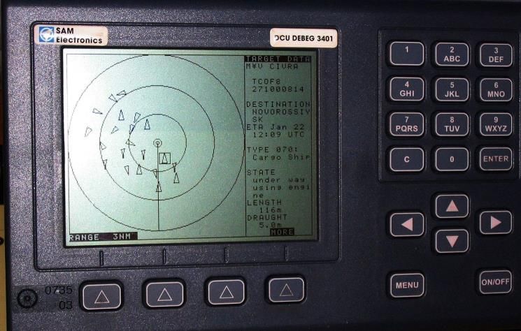
Figure 19: Distribution of arrival delay (measured in hours) for all ports, broken down by season of arrival
 A positive value indicates a delay, whilst a negative value indicates early arrival

3.3. Automatic Identification System (AIS)
AIS was first developed in the 1990s for use as a short-range identification and tracking system used on ships and
other marine traffic. On board AIS equipment (see Figure 20) allows ships to view traffic in their local area (10 to 20
nautical miles) and to simultaneously be seen by that traffic.

 Figure 20: On-board AIS equipment and typical graphical display

More recently the AIS system has been used to support:
• collision avoidance, notably amongst vessels outside the range of shore-based systems
• fishing fleet monitoring and control
• vessel traffic services, used to augment existing systems such as local vessel traffic service (VTS)

 17

• maritime security, to identify and monitor suspicious activity patterns
• aids to navigation, which may support or replace information generated by radar beacons currently used for
 electronic navigation aids
• search and rescue., coordinating on-scene resources of a marine search and rescue (SAR) operation
• accident investigation, AIS information is more accurate and comprehensive than transitional systems such as
 radar
• ocean current estimates
• fleet and cargo tracking

There are 27 types of AIS message. Of these, two are relevant to this report as they relate to ship position and
dynamics. Class A messages are sent by large ships typically over 300 tonnes and those carrying passengers. Class B
messages are used by lighter commercial and leisure craft. In both cases, an AIS transmitter will send the following
information every 2 to 10 seconds when underway and every three minutes when stationary or at anchor:
• Maritime Mobile Service Identity (MMSI) the unique ship identifier
• navigation status, at anchor, under way using engine(s), not under command an so on
• rate of turn, right or left, from 0 to 720 degrees per minute
• speed over ground, 0.1 knot resolution from 0 to 102 knots
• longitude, accurate to 0.0001 minutes
• latitude, accurate to 0.0001 minutes
• course over ground, relative to true north to 0.1 degrees
• true heading, 0 to 359 degrees
• true bearing at own position, 0 to 359 degrees
• UTC seconds, the seconds field of the UTC time when the data were generated

Higher-level information is transmitted less frequently (every six minutes):
• Maritime Mobile Service Identity (MMSI), the unique ship identifier
• radio call sign, up to seven characters
• name of vessel
• type of ship and cargo
• ship dimension
• location of positioning system (such as GPS) antenna on board the vessel
• type of positioning system – such as GPS, DGPS or LORAN-C
• draught of ship – 0.1 to 25.5 metres
• intended destination
• ETA, estimated time of arrival at destination

A recent development of the AIS system is the ability to make it viewable on the internet without the need for a
dedicated receiver. This removes the range limitation of the marine-based receivers and allows AIS data to be
visualised over a wider area (see Figure 21). With permission, data may also be downloaded to be used for additional
offline processing.

 18

Figure 21: Online AIS data showing the position of ships around the UK at noon on the 25 April 2018

3.4. Processing AIS data
The AIS data used for this study spans for a period of 12 months, between 1 August 2016 and 31 July 2017. The raw
data encoded using the National Marine Electronics Association (NMEA) format, was approximately one terabyte in
size and consisted of almost three billion rows. A Hadoop Distributed File System (HDFS) environment was used to
decode the encoded messages, process the new data, filter out the required types of messages and extract smaller
slices of data based on certain criteria, as described in the next subsections.

Once the data was saved in the HDFS environment, it was accessed using Pig, Hive and Spark as part of the Hadoop
stack. Decoders for individual types of message were written in Scala (see next section), the raw data was decoded
in a table format and saved as Parquet files. Scala functions were also developed to filter out the data based on the
type of message, unique ID of ship, timestamp, geographic location and other criteria. After filtering, the data was
extracted from the Hadoop environment, stored in local machines and further processed using Python and R (see
Figure 22).

 19

Figure 22: Cloudera distributed system environment

3.5. Decoding AIS data
AIS data was extracted in standard National Marine Electronics Association AIS message format; this is a text encoded
binary format that was decoded before being split into a series of files based upon the AIS message type. As some
messages are split over multiple lines (see Figure 23), they were concatenated before being decoded into real data
that can be directly interpreted and processed.

 Figure 23: One-line and two-line examples of raw AIS messages

The component of the positioning Type 1 AIS message that was of specific interest is:

 \!BSVDM,1,1,,A,E>jHCFbW7a:4@1Pa9@1:WdP0000Or:e=@6q@@10888uf:0,0*27

 20

The message is comma-separated with each element of the message decoding to a unique piece of information (Table
1).

 Component Description
 \!BSVDM The NMEA message type
 1 Number of message lines
 1 Sentence number (1 unless it´s a multi-sentence message)
 Sequential message ID (for multi-sentence messages)
 A AIS Channel (A or B)
 E>jHCF... Encoded AIS data
 0* End of data terminator
 27 NMEA checksum

 Table 1: AIS decoded message components
 (NMEA provide a full review)

Message integrity was checked using the NMEA checksum and corrupted messages discarded. The multi-sentence
messages were then assembled together into single messages, through concatenation of the encoded AIS data parts.
In NMEA AIS encoding, each ASCII character corresponds to six binary bits (unlike normal ASCII which uses eight). To
account for this, the decoding algorithm steps through each character of the encoded AIS data and subtracts 48 from
the decoded value. If the resulting number is a decimal number with a value greater than 40, the algorithm again
subtracts eight. The resulting number is then converted to a binary string that is split into substrings using the message
element positioning given in the NMEA encoding specification. Table 2 provides samples of the relevant splitting
positions for an AIS message.

 Element Position
 MMSI Number from bit 8 for 30 bits
 Longitude from bit 61 for 28 bits
 Latitude from bit 89 for 27 bits
 Course from bit 116 for 12 bits
 Heading from bit 128 for 9 bits

 Table 2: AIS message splitting positions

The data was finally split according to the message type and saved in intermediate storage. During saving, the data
was partitioned according to the time stamp of the AIS message. The parquet storage format was used as it offered
good compression, incremental addition of new data, most importantly, the ability to read only specified segments
instead of the full dataset.

One important feature that was considered when processing the AIS data was the ability to extract the messages
within a specified time window and for a specific area of interest. The area of interest was defined as a rectangular
geometric shape specified by the latitudinal and longitudinal coordinates of the top-left and bottom-right corners.
The data was read from the compressed parquet storage format using predicate pushdown based on the requested
time window and filtered in a distributed manner based on the coordinates for each message. Then the data was
collected into the driver node and exported in comma-separated values (csv) format.

All the above procedures were developed within the Apache Spark distributed computing engine and the data was
stored in Apache Hadoop. For this project, only data from the waters around the UK was used, however the linear
scalability of the distributed computation and storage allows the algorithm to be easily applied to data at a global
scale.

 21

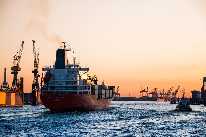
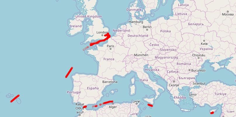
3.6. Visualising AIS data
Once the AIS data has been decoded into a series of latitude and longitudinal pairs it can be plotted and superimposed
onto a map or nautical chart. These plots can be used to gain an understanding of ship positions at a given point in
time and ship movements across any given time window.

 Figure 24: AIS base-station data for a single ship

Figure 24 gives the AIS track for a single Liquefied Natural Gas (LNG) tanker6. The diagram shows that ship travels
through the Azores (bottom left of the chart) into the English Channel and docks in London Medway port. The ship
then leaves port and once again passes through the English Channel, before heading south past the north-western
tip of Spain. The ship turns east and then continues its journey through the Strait of Gibraltar on through the
Mediterranean, finally docking in Cyprus.

It should be noted that the gaps in the base-station data relate to missing AIS coverage caused by the ship being
outside the range of ground stations. In such cases, AIS coverage is maintained by using satellite tracking. As all UK
ports and their surrounding waters are within range of at least one base station, AIS coverage is complete in the data
used for this project.

One particular area of interest in the voyage of this tanker can be seen due east of London Medway port (Figure 25).

6
 The data for this was provided by Centre for Big Data Statistics at Statistics Netherlands (CBDS) and did not form part of the
data extract used for the remainder of the project.

 22

Figure 25: AIS base-station data for a single ship (enlarged view)

One may reasonably expect that the tanker would follow a smooth arching path starting north-east through the
channel and turning onto a south-westerly bearing into port. However, the ship comes to a stop and remains
stationary for several hours (circled), before heading away from port on a due north heading before turning through
180 degrees and travelling south-west into port. Conversation with domain expert have indicated that this behaviour
is indicative of the ship waiting for cargo price to increase before it enters port and docks. Although the behaviour of
the above tanker may appear counterintuitive in open sea, it becomes more consistent as it approaches port, as the
ship enters and leaves in a more uniform manner. However, this consistency is not observed in all ports.

 Figure 26: AIS base-station data for a single ship (port of Rotterdam)

 23

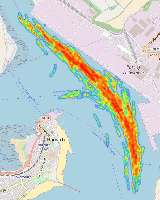
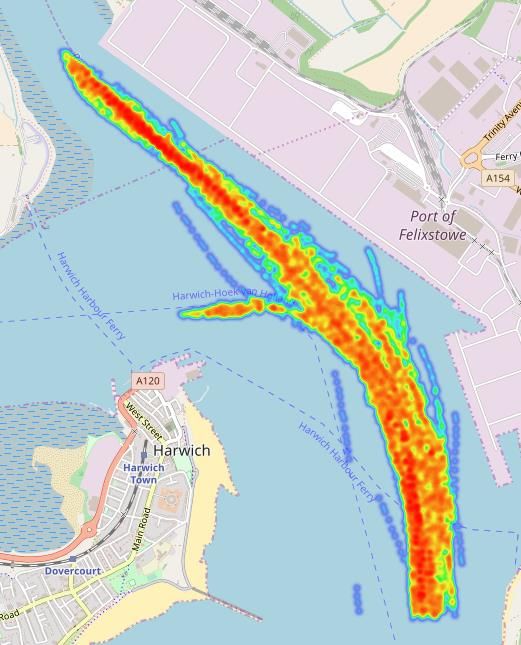
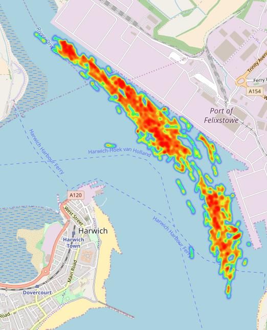
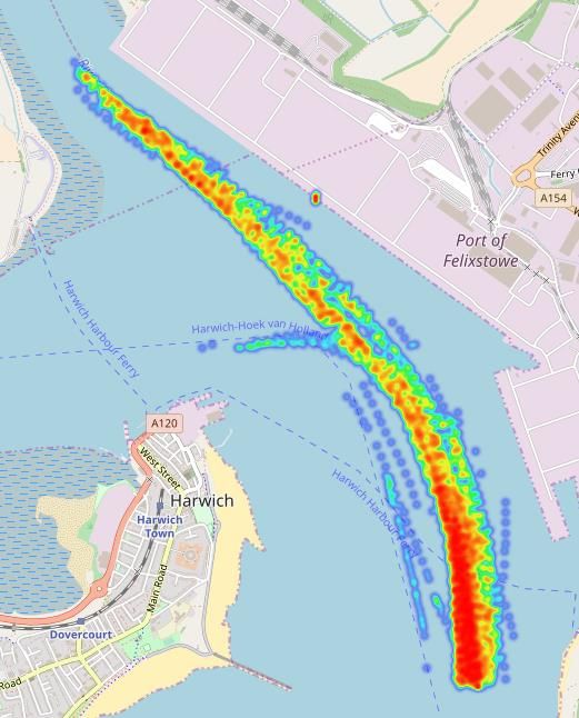
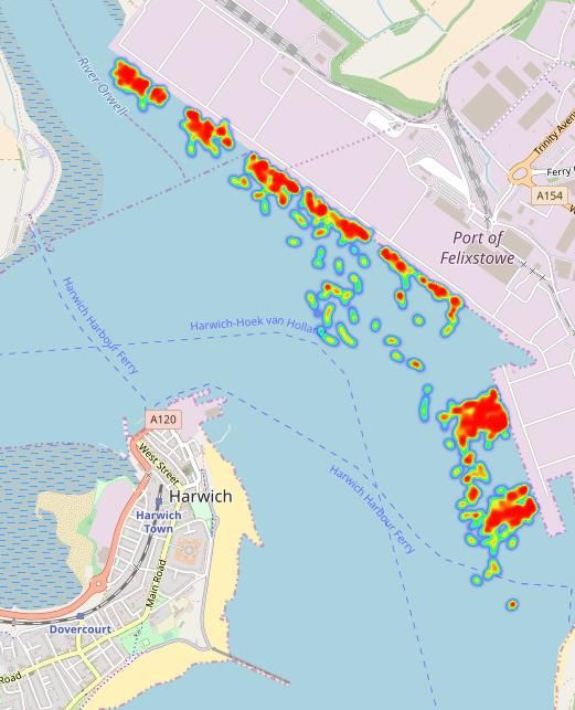
Figure 26 shows the journey of a light general transporter in and around the port of Rotterdam7. Unlike the LNG
tanker discussed earlier, the ship in this instance calls at several berths within the port, loading and unloading cargo
throughout.

A final example is discussed below. The tracks relate to several journeys undertaken by a large 200,000 tonnes, 400m
by 60m container ship within the port of Felixstowe. The highlighted area illustrates that on at least two occasions
the tanker heads north before turning sharply through 180 degrees and heading south before docking at a berth it
had previously travelled past (see Figure 27). On first inspection this behaviour may appear unexpected, however it
is an accepted practice for a docking ship to manoeuvre against the prevailing inbound current caused by the flooding
tide to aid the docking process.

 Figure 27: AIS base-station data for a container ship

To this point, AIS data has been used to explore the voyages of individual ships. However, the daily points taken from
within an area can be combined to produce a heatmap of ship movements within a port. This can be used to indicate
shipping lanes, port berths and port loading over time.

Figure 28 highlights notable features relating to Felixstowe (the busiest container port in the UK), including:
• the emergence of “hot” regions indicating unique berths within the northern edge of the port, most notably on
 12 December and 1 January
• evidence that not all ships that enter Felixstowe go on to dock at the port, some ships turn east and head towards
 the international port of Harwich whilst others head north west onto the river Orwell and onto inland destinations
• port loading on Christmas day is considerably lower than on other days

7
 The data for this was provided by Centre for Big Data Statistics at Statistics Netherlands (CBDS) and was not part of the data
extract used for the remainder of the project

 24

Monday 12 December 2016 Monday 19 December 2016

 Sunday 25 December 2016 Sunday 1 January 2016

Figure 28: Port loading, Felixstowe (from green, through amber to red represents an increasing density of AIS
 points)

 25

4. Classifying AIS data
The previous section presents examples of how the visualisation of AIS tracks within a given port and on the open sea
can be used to support the high-level understanding of ship and port behaviour on a macro level, for example,
identifying shipping lanes, holding areas, port berths, port loading and so on. However, this visually driven approach
is of limited use in quantitatively classifying behaviour on an individual ship-by-ship basis. To address this, various
machine learning techniques were applied to the AIS data to extract actionable insight. An unsupervised k-means
classifier8 was used to segment the behaviour of a ship into one of many intuitive states (transitioning through port,
manoeuvring into dock, docked and so on). These behavioural states transform the AIS data to a more meaningful
and interpretable representation which can be used to better understand the behaviour of a ship at any point on its
voyage.

AIS data was extracted from the port of Felixstowe and its surrounding sea spanning a 12-month time window from
1 August 2016 to 31 July 2017. Several features within the AIS data were investigated as potential inputs to the
segmentation, these including:
• Speed over Ground (SOG) (knots)
• acceleration (derived from SOG) (knots per second)
• Rate of Turn (ROT) (degrees per second)
• bearing (degrees)
• heading (degrees)

It is critical that any classification should be sufficiently robust so that it may be applied to the ships at any port or at
any geographic area in open sea. Early investigations showed that a segmentation using either bearing or heading as
features, although powerful from a classification perspective, would fail from the standpoint of robustness. Consider
a segmentation trained upon the data from ships operating in and around the port of Southampton on the south
coast of England. It follows that a ship heading into dock would predominantly be heading in a northerly direction.
During training, the machine learning algorithm would learn that ships heading north would be entering port whilst
ships heading south would be leaving port. If this pre-trained segmentation was then applied to a port on the north
coast of Scotland where ships head south to enter port and north to leave port, the segmentation would clearly
classify incorrectly. The impact of this could be mitigated to a degree by sampling AIS tracks from ports at different
orientations; however, the problem would not be completely removed since UK ports do not cover every possible
orientation.

 -720 0 720 -50 0 50
 Between -720 and 720 degrees per minute Between -50 and 50 degrees per minute
 Figure 29: Distribution of ROT

8
 Kmeans clusters aims to find similar groups or segments within the data, with the number of groups represented by the
parameters k. It works by iteratively assigning each data point to one of k groups based on the features that are provided. Data
points are clustered based on feature similarity (MacQueen, 1967).

 26

As speed over ground (SOG) and rate of turn (ROT) do not suffer from these drawbacks they were chosen as more
suitable inputs to the segmentation. On closer inspection, the distribution of the ROT variable taken directly from the
AIS sample did not follow the expected normal distribution - a large proportion of records are located at very large
ROT values (see Figure 29).

A new ROT variable was derived directly from the latitudinal and longitudinal points as shown below.

 High ROT
 t3
 θ
 t2 Low ROT

 t1

 θ
 ROT =
 (t3 – t2)

 Figure 30: Calculating ROT

Figure 30 shows three latitudinal and longitudinal pairs that describe positions on the sea at times t1, t2 and t3. The
ROT at t2 is given by firstly calculating the angle of turn  at t2 using standard trigonometric techniques. This angle is
then divided by the time taken to travel between t3 and t2 to give ROT. The two ship tracks on the right-hand side
illustrate the differences between high and low ROT.

A kmeans clustering algorithm was applied to training data containing SOG and ROT pairs taken in isolation at every
point along the track of each ship (Figure 31). In this instance, if the voyage of a single ship contains 1,000 AIS points
all 1,000 points were used for training purposes.

To remove noise created by smaller ships such as tugs and ferries, AIS data was extracted for the following ship types:
• container ship
• general cargo ship
• chemical and oil product tankers
• cargo ship
• bulk carrier

This reduced the number of available AIS data points from 10.1 to 2.3 million, corresponding to 772 unique ships.

 27

TP7

 TP6
 TP5
 TP4
 TP4
 TP3
 TP2 TPn - nth training data point
 TP1

 Full journey

 Figure 31: Training data for a single ship
 (Simplified for clarify, in reality each ship journey contains many more AIS data points)

The approach identified several unique segments. However, most identified segments were noisy with very few
containing unique or intuitive behaviours. As this approach treats each AIS data point in isolation, with no
consideration given to the relationship between points over time, it is overly sensitive to noise within the AIS data,
caused by atmospheric effects, obsolete equipment or on-board interference. A more robust approach was
developed that added a time-based aggregated component to the SOG and ROT fields that reduces the sensitivity of
the segmentation to AIS signal noise. For each journey, a random slice of AIS data was taken during the voyage (see
Figure 32). Several different time windows we investigated ranging from one to 10 minutes. A two-minute slice was
found to give the best balance between sensitivity and robustness.

 TP2

 TP1

 TP3

 TPn - nth training data point
 Full journey Slice 1 Slice 2 Slice 3
 Figure 32: Three random journey slices taken from the path of a single ship

 28

Histograms of the SOG and ROT values were then created and converted into two state vectors, SOG and ROT.
 Essentially, each state vector represents a historical distribution of the individual SOG and ROT values across the
 preceding two minutes. The bin boundaries for the SOG and ROT state vectors were selected to ensure approximately
 equal quantile population density across the entire training dataset. The final boundaries are given in Table 3,

 Quantile Range
 1 SOG = 0 Quantile Range
 2 0 < SOG ≤ 1 1 ROT ≤ 0.1
 3 1 < SOG ≤ 2 2 0.1 < ROT ≤ 0.6
 4 2 < SOG ≤ 3 3 0.6 < ROT ≤ 2.5
 5 3 < SOG ≤ 5 4 2.5 < ROT ≤ 8
 6 5 < SOG ≤ 10 5 ROT > 8
 7 SOG > 10

 Table 3: Bin boundaries for SOG and ROT

Figure 33 gives the ROT and SOG state vectors for a given point (TP1) on a hypothetical voyage. In this example the ROT
distribution assumes an approximate log normal distribution whilst the SOG distribution is exponentially distributed, it
can therefore be concluded that in the preceding two minutes this ship is generally travelling at lower speeds and with
limited rate of turn.

One disadvantage of this approach stems from the fact that the data is aggregated over all the AIS points within a two-
minute window. If only one slice is taken from each ship voyage then the resulting training data-set will be significantly
smaller than that generated in the previous approach. To overcome this, several random slices are taken from each voyage
to maintain approximately consistent training dataset sizes.

 3
 തതതതതത 1 = 0.13 0.38 0.25 0.13 0.13
 
 2
 1
 1 1

 TP1 ROT
 0 

 5

 4 തതതതതത
 1 = 0.28 0.22 0.17 0.11 0.11 0.06 0.06
 3

 2 2
 Hi Hi 1 1

 SOG
 0 

 Figure 33: The SOG and ROT state vectors for a given journey slice

 29

As with the previous approach, a k-means unsupervised algorithm was applied to the training data, the number of
generated segments (k) was set to an arbitrarily large value of eight. Segments that were similar based upon their centroids
as defined by the ROT and SOG state vectors were merged. This gave a final set of six unique segments. These segments
were each assigned descriptive name to aid interpretation. Each of the six segments fall into the following three higher-
level behavioural groups:
• transitional behaviour
• docking behaviour
• docked behaviour

The following section discusses each of the six segments in turn. In each case, a table indicates where each segment over
indexes (green) within the SOG and ROT input state vectors. A heat map then gives all the AIS points that fall into each of
the segments (each percentage value gives the number of training points that fall into that segment).

Transitional segments
Ships within the two transitional segments (Figure 34) do not dock within the port and are not in the process of docking.
Instead they use the port to transition into other inland areas. In the case of Felixstowe this is either heading east to the
port of Harwich or north-west to other inland destinations.

 Speed over Ground (SOG) Rate of Turn (ROT)
 0 0-1 1-2 2-3 3-5 5-10 10+ 0.1 0.1-0.6 0.6-2.5 2.5-8 8+
 Border phase
 General phase

 Border phase General phase
 (4% of training dataset) (57% of training dataset)

 Figure 34: Transitional segments, (from green, through amber to red represents
 an increasing density of AIS points)

 30

The border phase segment has the highest speed of all segments, its ROT is typically low indicating that ships in this
segment are not manoeuvring to any significant degree. The heatmap shows that there is a higher density of points located
around the southern border of the port. It is suggested that this segment represents ships that are entering port and
slowing down from their open-water cruising speed to the speed limit within the port. The general phase segment is
closely related to the border phase segment. Although the ROT distributions are similar, the speed of the ships in this
segment is significantly lower. This coupled with the heatmap, which shows no noticeable increase in density, suggests
that these ships have passed the port boundary and are observing the local speed limit whilst they transition through the
port.

One interesting feature of the border phase plot illustrates the noise that is sometimes present in the AIS data. The circled
point relates to the AIS reading from a ship that is positioned against the northern harbour wall. However, the SOG reading
for this point indicates that the ship is travelling at over 10 knots. This is clearly impossible and is likely to be caused by
noise within the AIS data, however the machine learning approach is robust enough to handle this and other data
anomalies.

Docking segments
The docking segments (Figure 35) classify ships that have initiated the process of docking into one of the harbour berths.
There are three docking segments, each one relates to a unique phase of the docking process.

 Speed over Ground (SOG) Rate of Turn (ROT)
 0 0-1 1-2 2-3 3-5 5-10 10+ 0.1 0.1-0.6 0.6-2.5 2.5-8 8+
 Initial phase
 Mid phase
 Terminal phase

 Initial phase Mid phase Terminal phase
 (10% of training dataset) (5% of training dataset) (13% of training dataset)

 Figure 35: Docking segments, (from green, through amber to red represents an increasing density of AIS points)

 31

The speed of ships within the initial phase segment has dropped below that of the transitional phase ships. Their AIS points
on the heat map indicate that they are turning towards the harbour berths. Ships classified within the mid-phase segment
have decreased their speed further and are also starting to manoeuvre into dock (indicated by increasing ROT values). The
final docking segment, terminal phase, is characterised by very slow speeds (less that one knot) and high ROT values. Ships
in this segment are in the final stages of docking and are turning into their intended berth at very slow speeds and higher
rates of turn. The heatmap for this illustrates the vicinity of the ships to the harbour wall.

Docked segment
The final segment relates to ships that have reached their destination (Figure 36). Ships within this segment have virtually
no speed, the high rates of turn relate to the very final stages of the docking process where final adjustments are made to
the ship position within the port. This heatmap for the segment confirms that the ships are all docked or very close to
being so.

 Speed over Ground (SOG) Rate of Turn (ROT)
 0 0-1 1-2 2-3 3-5 5-10 10+ 0.1 0.1-0.6 0.6-2.5 2.5-8 8+
 Docked

 Figure 36: Docked segment (12% of training dataset)

In an attempt to further distinguish between ships entering and leaving port and dock, the segmentation was expanded
to include a deceleration feature. This feature was pre-processed in exactly the same way as the SOG and ROT features.
It was found that the acceleration feature dominated the segmentation and washed out the contribution of both the ROT
and SOG features resulting in its removal for subsequent analysis.

Recall that the inputs to the segmentation algorithm are two state vectors consisting of a total of 12 values. The centroid
of each of the six segments can be defined within 12-dimension space. An informative exercise is to visualise the six
segment centroids in two-dimensional space so that the spatial separation of each segment may be explored. This is
achieved by applying t-distributed Stochastic Neighbour Embedding (t-SNE)9. Figure 37 gives the result of applying t-SNE
to the six segment centroids.

9
 t-SNE is a dimensionality reduction technique that is especially suited to reducing high-dimensional data into a space of two or three
dimensions (van der Maaten et. al. 2008)
 32