Data Driven Insight Into Fish Behaviour and Their Use for Precision Aquaculture
←
→
Page content transcription
If your browser does not render page correctly, please read the page content below
ORIGINAL RESEARCH
                                                                                                                                                   published: 28 July 2021
                                                                                                                                         doi: 10.3389/fanim.2021.695054

                                             Data Driven Insight Into Fish
                                             Behaviour and Their Use for
                                             Precision Aquaculture
                                             Fearghal O’Donncha 1*, Caitlin L. Stockwell 2 , Sonia Rey Planellas 3 , Giulia Micallef 4 ,
                                             Paulito Palmes 1 , Chris Webb 5 , Ramon Filgueira 6 and Jon Grant 2
                                             1
                                              IBM Research Europe, Dublin, Ireland, 2 Department of Oceanography, Dalhousie University, Halifax, NS, Canada, 3 Institute
                                             of Aquaculture, University of Stirling, Stirling, Scotland, 4 Gildeskål Research Station, Inndyr, Norway, 5 Cooke Aquaculture,
                                             Orkney, United Kingdom, 6 Marine Affairs Program, Dalhousie University, Halifax, NS, Canada

                                             Aquaculture, or the farmed production of fish and shellfish, has grown rapidly, from
                                             supplying just 7% of fish for human consumption in 1974 to more than half in 2016.
                                             This rapid expansion has led to the growth of Precision Aquaculture concept that aims
                                             to exploit data-driven management of fish production, thereby improving the farmer’s
                                             ability to monitor, control, and document biological processes in farms. Fundamental
                                             to this paradigm is monitoring of environmental and animal processes within a cage,
                         Edited by:          and processing those data toward farm insight using models and analytics. This paper
                 Suresh Neethirajan,
           Wageningen University and         presents an analysis of environmental and fish behaviour datasets collected at three
              Research, Netherlands          salmon farms in Norway, Scotland, and Canada. Information on fish behaviour were
                       Reviewed by:          collected using hydroacoustic sensors that sampled the vertical distribution of fish in
                    Isabella Condotta,
                                             a cage at high spatial and temporal resolution, while a network of environmental sensors
                 University of Illinois at
   Urbana-Champaign, United States           characterised local site conditions. We present an analysis of the hydroacoustic datasets
         Matthew Whitney Jorgensen,          using AutoML (or automatic machine learning) tools that enables developers with limited
 Agricultural Research Service, United
    States Department of Agriculture,        data science expertise to train high-quality models specific to the data at hand. We
                         United States       demonstrate how AutoML pipelines can be readily applied to aquaculture datasets to
                   *Correspondence:          interrogate the data and quantify the primary features that explains data variance. Results
                  Fearghal O’Donncha
                                             demonstrate that variables such as temperature, wind conditions, and hour-of-day were
                 feardonn@ie.ibm.com
                                             important drivers of fish motion at all sites. Further, there were distinct differences in
                    Specialty section:       factors that influenced in-cage variations driven by local variables such as water depth
          This article was submitted to
                                             and ambient environmental conditions (particularly dissolved oxygen). The framework
          Precision Livestock Farming,
                a section of the journal     offers a transferable approach to interrogate fish behaviour within farm systems, and
           Frontiers in Animal Science       quantify differences between sites.
              Received: 14 April 2021
                                             Keywords: machine learning, hydroacoustic, aquaculture, AutoML, IoT
              Accepted: 01 July 2021
              Published: 28 July 2021

                             Citation:
          O’Donncha F, Stockwell CL,
                                             1. INTRODUCTION
   Planellas SR, Micallef G, Palmes P,       1.1. Background
     Webb C, Filgueira R and Grant J
                                             Salmon fish farming started on an experimental level in the 1960s but became an industry in
  (2021) Data Driven Insight Into Fish
Behaviour and Their Use for Precision
                                             Norway and the UK in the 1980s, and in Chile in the 1990s (Laird, 1996). Global salmon production
                          Aquaculture.       is currently circa 2.4 Million Tonnes per annum in 2018 (FAO, 2020) with a market value of
          Front. Anim. Sci. 2:695054.        approximately 16 billion euros (Planet Tracker, 2021). Current production is mainly concentrated
    doi: 10.3389/fanim.2021.695054           in Norway, Chile, UK and Canada. The intensification of the salmon industry requires more specific

Frontiers in Animal Science | www.frontiersin.org                                    1                                               July 2021 | Volume 2 | Article 695054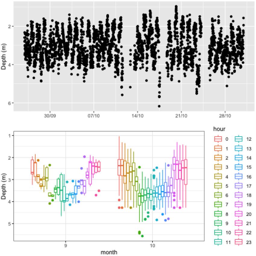
O’Donncha et al.                                                                                                           Data Driven Aquaculture

knowledge of the use of feed and the control and response to              changes in fish behaviour (i.e., variations in vertical motion and
the environment. The individual number of animals used in                 distributions). The contributions of the paper are as follows:
aquaculture has increased substantially over the last 3 decades.
                                                                          • We describe the monitoring, collection, and statistical
For example, only for Scottish aquaculture the number of fish
                                                                            analysis of environmental and hydroacoustic datasets at
transferred to sea increased from 25 million in 1990 to 47 million
                                                                            three salmon farms with very different environmental and
in 2018 (Marine Scotland Science, 2018).
                                                                            geographical characteristics.
    The use of big data and models to guide production in the
                                                                          • We outline an AutoML (or automatic machine learning)
agriculture space is well established, with initial implementations
                                                                            model development pipeline (data curation, preprocessing,
of precision agriculture, or information-based management
                                                                            and model setup) to train and deploy a machine learning
of agricultural production systems beginning in the 1980s.
                                                                            model to forecast fish behaviour using a “no-code” paradigm.
The fundamental approach reduces to leveraging data from
                                                                          • We present a framework to interrogate the trained model and
disparate sources (satellite, sensor arrays, image data, etc.)
                                                                            extract insight into the environmental drivers of fish behaviour
to guide decision and apply treatment in the right place at
                                                                            using explainable machine learning techniques. We discuss the
the right time. While precision agriculture originated with
                                                                            results of the data driven interrogation of fish response against
crop productions, applications related to livestock farming
                                                                            known drivers of fish behaviour from literature.
subsequently blossomed. These generally related to leveraging
various sensor technologies to monitor health and productivity            The objective of the paper was to develop a transferable
of livestock. Examples include radio frequency identification             approach to interrogate caged salmon behaviour and inform
(RFID) tags to identify cattle in computer-controlled feeders,            farm management. Results indicate that data-driven approaches
milking robots that ease the work of dairy operators, and                 have great promise to provide automated insight into fish
automatic milk feeders that customise the milk supplement for             behaviour, and the environmental conditions that influence that
calves, measure body weight and body temperature and generate             behavioural response. However, the analysis needs to be informed
reports (Gebbers and Adamchuk, 2010).                                     by domain expertise from ecology and fish welfare to allow a
    Precision aquaculture on the other hand is a nascent                  robust interpretation of results.
management concept that requires adoption of technologies                    The paper is structured as follows: below, we present a
from both crop and livestock management systems. Namely, an               detailed overview and literature review of fish behaviour and how
effective aquaculture management system needs to understand               information on fish movement and vertical distribution provides
the environmental conditions and the conditions of fish within            insight into behavioural and welfare aspects. Section 2 describes
that cage. Modern fish farms are comprised of cages with up               the study sites, introduces the machine learning approaches
to 200,000 fish. As farms are typically composed of 10–20                 used, and outlines the data curation and analysis framework.
cages, and multiple farms are often co-located in a bay, the              Section 3 presents results from this study while finally, we outline
total number of individual fish is enormous. This precludes               conclusions from this research and makes recommendations for
the direct translation of concepts from livestock farming, and            further work.
in practise, precision aquaculture is a marriage of approaches
developed for both precision livestock and grain cultivation,             1.2. Behaviour
i.e., fish are not managed as individuals as are cows, yet                Many studies of fish behaviour are in the wild or under controlled
are obviously more complex in management than plants                      laboratory conditions. Few of them have been done under farmed
(O’Donncha and Grant, 2019).                                              conditions mainly due to the challenges and multiple restrictions
    There has been extensive literature on observing, modelling           this production systems poses to the researchers (Johansson
and quantifying the environmental conditions of aquaculture               et al., 2006, 2014). However, a greater understanding of the
systems to inform on aspects such as site carrying capacity               role of fish behaviour as a key health and welfare indicator is
(Ferreira et al., 2013), environmental impacts (Buschmann                 essential to allow more autonomous monitoring of fish health.
et al., 2006), and mitigation activities to reduce environmental          The importance of fish behaviour as a farm management tool
footprint (Costa-Pierce, 2003). These class of studies contribute         has spurred interests in new technologies to monitor and
to the first pillar of precision aquaculture; of equal importance         infer behaviour such as sonar and video images or the use of
is monitoring and extracting insight on fish behaviour to inform          artificial intelligence.
operations. In this paper, we investigate fish behaviour within a
cage using hydroacoustic sensors. These datasets provide high             1.2.1. Salmon Aquaculture
resolution estimates of fish motion at the biomass (or group)             Many different biological, environmental and social parameters
level, and allow inference on fish behaviour and implications for         influence the behaviour of salmon when farmed in sea cages.
farm management. Such data and the information they provide               Parasites, such as sea lice, are a biological example that can
can be fundamental to empowering precision aquaculture and                cause behavioural changes to farmed salmon in order to combat
data-driven decision making.                                              infestation (Bui et al., 2016). Sea lice are concentrated near the
    This paper presents an analysis of environmental and                  surface, and methods to limit fish surface time have been a
hydroacoustic data from three salmon farms in Norway,                     focus of farm mitigation activities. Salmon have been observed
Scotland, and Canada. We use statistical and machine learning             to prefer deeper depths once highly infested to avoid further
approaches to interrogate the primary environmental drivers of            infestation (Bui et al., 2016). Temperature and dissolved oxygen

Frontiers in Animal Science | www.frontiersin.org                     2                                        July 2021 | Volume 2 | Article 695054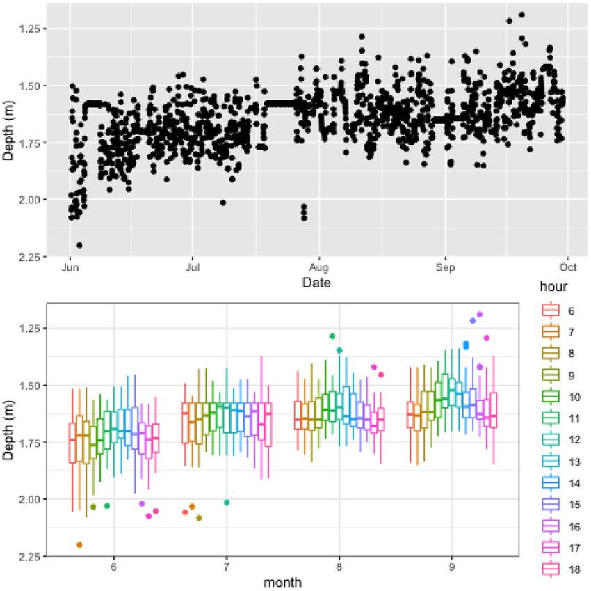
O’Donncha et al.                                                                                                          Data Driven Aquaculture

(DO) are an example of environmental parameters that affect               and the external environment can be a highly reliable and non-
the behaviour of Atlantic salmon. For example, Atlantic salmon            invasive operational welfare indicator (OWI) (Martins et al.,
will distribute themselves according to preferred temperature             2011; Damsgård et al., 2019). A key area of research for the
range, 8–18◦ C, with changes in behaviour occurring above and             industry is whether sensor observations such as these can be
below the threshold (Johansson et al., 2006, 2009; Oppedal                used to augment welfare indices, thereby reducing the necessity
et al., 2011). Similarly, DO is an important parameter affecting          to collect cumbersome manual samples such as lice counts and
fish behaviour as concentrations below the optimal range cause            gill health.
physiological stress and related behavioural changes such as a                Traditional methods of in situ observations of fish behaviour
reduction in feeding (Dempster et al., 2016; Oldham et al., 2018).        include visual inspections of the fish through random sampling,
Light intensity is another major contributor to fish behaviour            and video cameras placed in the feed zone of cages (Føre
by changing vertical distribution. During daylight hours, when            et al., 2018). Visual inspections are difficult to achieve on large
light intensity is at its greatest, fish tend to swim deeper in net       populations and can be stressful to the fish (Martins et al.,
pens to avoid surface predators (Fernö et al., 1995; Oppedal              2011). Video cameras can help identify when feed falls below
et al., 2001). It has been hypothesised ascent toward the surface         the depth of the camera indicating the fish within the cage are
during nighttime is a photo-regulatory behaviour to maintain              satiated. Although these videos provide real-time images, they
schooling as light fades. Furthermore, seasonal variation in light        only supply a small frame of the cage and are hindered by
availability changes vertical distribution with winter swimming           the challenge of capturing high quality images underwater. In
depths generally shallower than summer swimming depths (Juell             order to study behaviour on the cage’s population, a larger view
and Westerberg, 1993; Oppedal et al., 2001). However, this diel           of the cage is required. One suggested method of continuous
seasonal pattern changes when surface mounted artificial lights           observations includes a commercial system, CageEye (2021).
are installed in net pens (Oppedal et al., 2001). Populations have        CageEye is a hydroacoustic sensor which is placed in the
also been observed to remain in the upper half of net pens, under         cage and captures (in real-time) the relative density of fish in
normal stocking densities, to avoid large piscivorous fish present        the water column. Previous studies (Juell et al., 1993; Lindem
under net pens (Fernö et al., 1995; Juell and Fosseidengen, 2004;         and Houari, 1993) have investigated the effectiveness of using
Johansson et al., 2006, 2009; Dempster et al., 2016; Føre et al.,         CageEye to completely automate feeding by using the detection
2017). Additionally, hydrodynamic conditions, such as waves               of fish depth as indication of appetite. However, the use of this
and currents, will affect vertical distribution with stronger waves       technology has potential to be used to study fish behaviour and
encouraging fish toward the surface (Johannesen et al., 2020).            indirectly welfare.
    A group of fish that voluntarily remain together, or a shoal,             The association between behaviour and welfare can be
will have social group behaviour (Martins et al., 2011). A shoal          determined for Atlantic salmon by understanding abnormal
will adopt a polarised swimming pattern in order to minimise              behaviour as it is linked with stressors (Martins et al., 2011;
the possibility of collisions and by synchronising these patterns         Damsgård et al., 2019). Therefore, continuous monitoring of
a shoal can be deemed a school (Oppedal et al., 2011). Within a           fish behaviour can provide a more comprehensive perception
school there are rules in which all individuals must follow, and          of environmental conditions and their effect on welfare. The
deviations from these rules by one or a few individuals can result        description, classification, and understanding of fish movement,
in a group reaction. As with any population, individuals within a         as well as the environmental stimuli responsible for that
school will react differently when placed under the same stressors.       behaviour could become the foundation for the creation of
For example, one fish may be more motivated by feed and swim              an early-warning system of fish welfare. This early-warning
toward the surface while another may be content waiting for feed          system can trigger changes in aquaculture practises that result in
to fall. These individual differences can affect the behaviour of         improved welfare conditions for farmed fish.
the whole of the shoal regarding the responses to environmental               There are numerous studies dedicated to using machine
parameters or other external or internal stressors. The internal          learning to characterise and manage animal behaviour in
state of the fish is also an important parameter to consider to           agriculture (Liakos et al., 2018). These include automated
understand the fish behavioural responses (Castanheira et al.,            monitoring systems based on video camera (Matthews et al.,
2017; Damsgård et al., 2019). Internal states being the final             2017), and prediction of bovine weight trajectories based on
behavioural decision maker for the animal to respond to external          historical data (Alonso et al., 2015). Faced with a more
stimulae (Huntingford et al., 2011).                                      difficult monitoring environment, applications of machine
                                                                          learning to aquaculture have developed slower. Many studies
1.3. Related Work                                                         have investigated how machine learning could improve ocean
Technology on farms has increased significantly in the past               monitoring and forecasting either by mining large ocean
decade (Føre et al., 2018), and ongoing efforts focus on the              datasets Gokaraju et al. (2011) or relating future conditions
improvement of fish welfare and optimisation of farm operations,          to historical observations (Wolff et al., 2020). More recently,
e.g., minimising the waste of feed. Sensors such as real-time             the applications of machine learning and computer vision
oxygen and temperature probes, or acoustic tracking of fish               technology to aquaculture is receiving a lot of attention. Broadly
are becoming more common in fish farming. The use of                      these are applied across two categories: 1) pre-harvest and
hydroacoustic sensors to infer the behavioural response of the            during cultivation, and 2) post-harvest (Saberioon et al., 2017).
fish to the physical structure of the cage, aquaculture practises,        In the pre-harvest and cultivation stage, much of the research

Frontiers in Animal Science | www.frontiersin.org                     3                                       July 2021 | Volume 2 | Article 695054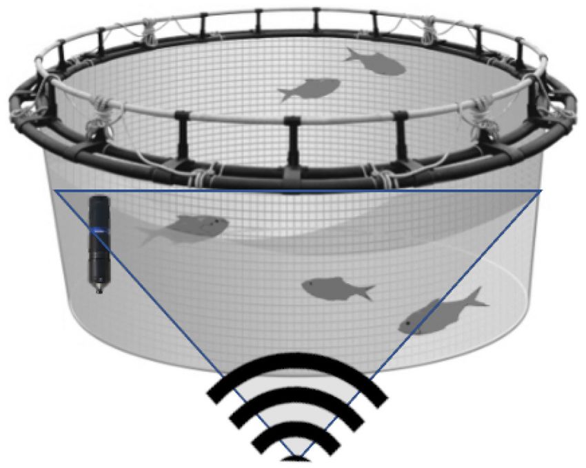
O’Donncha et al.                                                                                                           Data Driven Aquaculture

focuses on monitoring fish behaviour. A number of studies                   2.1.1. Norway Site
have demonstrated accurate monitoring of fish behaviour and                 The Norwegian site at Røssøya Nord (coordinates: 67◦ 4.38′
trajectory (Kato et al., 2004; Pérez-Escudero et al., 2014),                N 13◦ 56.855′ E) is a commercial farming site owned by
although these have been predominantly laboratory-based.                    GIFAS in Gildeskl municipality (Nordland, Norway). The site
Monitoring and optimising feeding activities using computer                 has a mooring system with placements for 16 cages (cage
vision and machine learning is an active area of research                   circumference 90 m; maximum cage depth 27 m). Seven cages
(Atoum et al., 2014). However, these provide little information             (circumference 90m, max depth 20 m) were stocked with 18G
about behavioural dynamics during feeding and are still at an               S1 smolt produced at Salten Smolt AS and Helgeland Smolt AS
early stage of development (Oppedal et al., 2011; Saberioon                 in August/September 2018. Smolt were transferred at an average
et al., 2017). Saberioon et al. (2017) provides an excellent                weight of 61 g (Salten) and 122 g (Helgeland) and each cage was
review of applications of computer vision and machine learning              stocked with approximately 150,000 smolt. The fish density at
technologies to aquaculture.                                                stocking was 1.3–2.1 kg/m3 .
                                                                               All the cages were fed on a standard commercial diet (EWOS
                                                                            Robust). Feed was delivered from the silos on the barge to the
                                                                            cages via an air-blowing system and into a rotor spreader at the
2. MATERIALS AND METHODS                                                    cage surface. Feeding start time, feeding intensity, and number
                                                                            of meals were adjusted according to day-length, weather, and
Hydroacoustic methods provide a proxy measure for density and               observations on fish behaviour by the site staff.
distribution of marine animals in form of acoustic backscattering              A designated cage was instrumented to explore environmental
(Foote, 2009). The fundamental principle is based on emitting               variations and fish distribution (hydroacoustic sampling)
a signal of known type and power level from a transducer. As                between 20/02/2019 and 800 is a numerical ocean 31/10/2019.
it encounters regions of the medium with differing properties,              During the experiment it was decided to change the fish stock
also called heterogeneities, the sound is generally redistributed,          since they were not growing optimally. Therefore, the stock
or scattered, in all directions. This makes possible detection of the       were replaced with 50,000 fish supplied by Helgeland Smolt in
scattered sound with transducer and suitable receiver electronics.          July 2019. The fish density after the change in fish stock was
Advantages linked to hydroacoustic sampling techniques include,             10.1 kg/m3 .
high spatial and temporal resolution, autonomous long-term                     Environmental variables were measured by Aanderaa
sampling duration, range (especially during poor visibility when            instruments (Xylem analytics, Norway). The variables measured
visual-based methods tend to fail), and a non-invasive surveying            were salinity, temperature, DO, as well as current speed
approach (Scherelis et al., 2020). Given these advantages,                  and direction. Animal variables were monitored by an
hydroacoustics is increasingly used to characterise animal                  Aquaculture Biomass Monitor sensor, ABM (Biometrics
behaviour in the marine environment, and considered a                       AS, Norway) which consists of a split-beam sonar mounted on
promising system to improve management of aquaculture farms                 a buoy and it can detect over 50,000 fish per day. The sonar
(Bjordal et al., 1993; Juell et al., 1993).                                 provided an estimate of total biomass, biomass distribution
    In this study, hydroacoustic data were collected by one of              with depth, fish weight distribution and fish swimming
two sensors “CageEye” (Scherelis et al., 2020) or “Aquaculture              speed. Fish position and distribution are reported hourly,
Biomass Monitor” ABM (2020). Broadly speaking, processed                    while estimates of average fish size are returned at multi-
hydroacoustic data generates two metrics: volume backscattering             day period. Figure 1 presents a schematic of typical sensor
strength (Sv ), is often considered as a proxy for fish biomass;            configuration within a cage. The hydroacoustic sensor was
while target strength (TS) is an acoustic measure of fish                   installed beneath the cage looking upwards. It sampled at an
length (Simmonds and MacLennan, 2008). TS is a measure of                   angle of approximately 42◦ from horizontal. An environmental
the acoustic reflectivity of a fish, which varies depending on              sensor was deployed at approximately mid-depth in
the presence of a swim bladder and on the size, behaviour,                  the cage.
morphology, and physiology of the fish. These outputs can be                   Since the environmental sensor deployment (May–July) did
used to generate estimates of fish density and biomass (Boswell             not cover the entire study period, we augmented environmental
et al., 2007) within a cage.                                                data with output from the NorKyst-800 ocean model (Albretsen
                                                                            et al., 2011). The NorKyst-800 is a numerical ocean modelling
                                                                            system deployed to simulate physical oceanography variables
2.1. Study Sites                                                            such as sea level, temperature, salinity and, currents for all
This study considers three salmon cage farms in Norway                      coastal areas in Norway and adjacent seas. The model has a
(NOR), Scotland (SCO), and Canada (CAN). For each site a                    horizontal resolution of 800 m, 35 layers in the vertical, and can
number of environmental sensors were deployed monitoring a                  be downloaded from the OPeNDAP server provisioned by the
range of parameters, including temperature, DO, and current                 Norwegian Meteorological Institute (Norwegian Meteorological
speed. These were complemented with weather data from in-                   Institute, 2021). The model provides a satisfactory representation
situ weather stations or model generated reanalysis from IBM                of Norwegian off- and onshore dynamics but requires higher
Environmental Intelligence Suite available through their public             resolution to resolve the dynamics of most Norwegian fjords
API IBM (2021b).                                                            properly (Albretsen et al., 2011).

Frontiers in Animal Science | www.frontiersin.org                       4                                      July 2021 | Volume 2 | Article 695054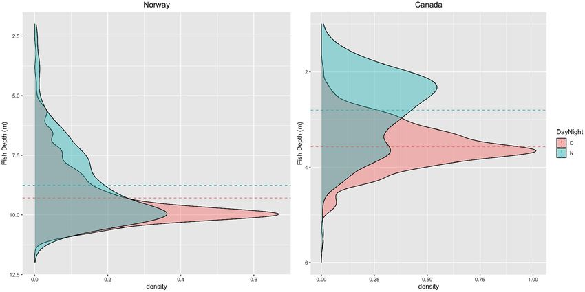
O’Donncha et al.                                                                                                                        Data Driven Aquaculture

                                                                                       record DO and temperature: a handheld underwater wireless
                                                                                       sensor (OxyGuard International, 2014) sampled daily from
                                                                                       08/01/2019 to 30/10/2019 and an in-situ Realtime Aquaculture
                                                                                       sensor (Innovasea, 2021) sampled at 10-min intervals at a depth
                                                                                       of 2.5 m from 13/11/2019 to 07/02/2020. As for the Norway site,
                                                                                       due to the difficulty to collect continuous environmental data
                                                                                       for the entire period, model data extracted from the Copernicus
                                                                                       Marine Service model repository augmented sensor datasets.
                                                                                       Temperature, DO, sea surface height (SSH), and current speed
                                                                                       were extracted from the Atlantic North West Shelf model at
                                                                                       the surface layer. Data is available at a 1.5 km (Tonani et al.,
                                                                                       2019) horizontal resolution at hourly intervals and can be freely
                                                                                       downloaded from the Copernicus portal. We compared sensor
                                                                                       and model data for the period and since the overall trends
                                                                                       were very similar, we augmented periods when sensor data
                                                                                       were missing with Copernicus data. We noted that the model
                                                                                       tended to overestimate magnitude of temperature, but since
 FIGURE 1 | Schematic of sensor configuration within a cage. The
                                                                                       they captured the temporal variations, it served to adequately
 environmental sensor is denoted in the left hand side of cage with the exact          represent conditions for machine learning purposes. It’s worth
 location varying across sites (e.g., for Norway it was deployed at 5 m depth in       noting that the ML model is not affected by data magnitudes
 centre of cage), while the hydroacoustic sensor and it’s sampling domain is           since data is normalised. Instead it learns how the predictand
 denoted beneath the cage (pointing upwards). Note, that the hydroacoustic
                                                                                       (label) varies in response to predictors (features). Using data from
 sensor contains sampling “blind spots,” especially toward the bottom of the
 cage which causes challenges in shallow sites where depth is limited. This            a physics model can be a pragmatic approach to handling missing
 figure represents an idealised representation of the deployment and naturally         values in environmental studies, thereby avoiding reliance on
 there are many practical considerations with regards sensor deployment                statistical imputation methods.
 (power source, ease of access, anchoring point, etc.).                                    The relative biomass distribution within the cage was assessed
                                                                                       using the beam sonar system, CageEye. The system in Orkney
                                                                                       was made up of an echosounder and one transducer. The
                                                                                       transducer was placed in the cage at a depth of approximately 5.5
2.1.2. Scotland Site                                                                   m, and connected to the echosounder cabinet, which was placed
The salmon sea farm is located at Carness Bay, Orkney                                  on the cage ring and sent the data wirelessly to the base station at
(coordinates: 59◦ 00.637′ N 02◦ 55.374′ W). This barge fed site                        the feeding barge. The transducer was placed as deep as possible,
includes a total of 12 × 100 m circumference cages and maximum                         looking up at most of the biomass of the cage. The transducer had
net depth of 6 m. The total number of fish stocked at the end of                       two angles that they switch between, approximately 14 degrees
January 2019 was approximately 230,000, with a stocking density                        (200 kHz) and 42 (50 kHz) degrees: this allowed one to get
of 5.1 kg/m3 . Fish stocked were 18S1 smolts, which were moved                         echogram recordings of both. It is important to note that this
from Meil bay to Carness Bay on 5th February 2019. Each cage is                        site did not have power at night, and consequently (since sensor
stocked with approximately 20,000 salmon.                                              did not have battery source), the acoustic sensor was switched off
   All the cages were fed on a standard commercial diet (Biomar,                       between 18:00 and 06:00.
power extreme). Feed was distributed to the fish cage from
the hulls on the barge via an air-blowing system. Feeding                              2.1.3. Canada Site
was controlled by AkvaConnect software (AkvaGroup AS).                                 The Canadian study site located in Saddle Island, Nova Scotia
Feeding started at pre-determined times according to day length,                       (coordinates: 44◦ 30.225′ N 64◦ 2.923′ W) is a commercially
most often with a meal duration of 30–60 min. The stock                                operated Atlantic salmon farm. The site had one column of 6
were monitored by camera and feeding intensity was adjusted                            cages measuring 150 m circumference and a maximum depth
accordingly. For example, should the fish exhibit poor feeding                         of 11 m. Each cage contained approximately 60,000 fish with a
activity, the feeding intensity would be decreased or stopped in                       stocking density of about 10 kg/m3 . Fish were fed twice daily, with
the affected cages. Adjustments in the feeding intensity were done                     the exact times dependent on daylight availability.
daily according to requirement and light availability. As soon                            Each cage was equipped with two RealTime Aquaculture
as there was enough light, the first meal started (lasting 30 min                      (Innovasea, 2021) probes deployed at 2 and 8 m depths. The
according to appetite), and fish were fed again after a pause of                       probes measured temperature and DO, while an ADCP profiler
4–6 h. A maximum of 2 meals were administered per day.                                 sampling current speed was deployed in the northeast corner of
   Cage 8 was instrumented to collect both environmental                               the farm. Sea surface height was extracted from the Copernicus
and animal variables i.e., variables concerning fish behaviour,                        portal, in similar manner to the other two sites. Two of the
growth and welfare data. Water temperature, DO, turbidity                              cages were equipped with a CageEye sensor from 11/09/2019
and salinity were measured for each cage daily by the site                             to 30/10/2019. Each system consisted of three transducers, with
management staff. Cage 8 was monitored with two sensors to                             two placed in opposite corners at 7 m depth, facing upwards,

Frontiers in Animal Science | www.frontiersin.org                                  5                                        July 2021 | Volume 2 | Article 695054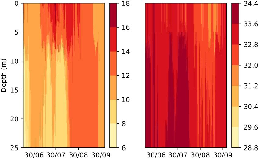
O’Donncha et al.                                                                                                                           Data Driven Aquaculture

TABLE 1 | Summary metrics for the three sites describing location, water depth,               As a benchmark, we compared results against a manually
cage depth, average tidal range, number of fish per cage, and fish density.                tuned machine learning model, namely Random Forest (RF).
                          NOR                  SCO                   CAN
                                                                                           RF is one of the most popular machine learning models and
                                                                                           has demonstrated excellent performance in complex prediction
Latitude                  67◦ 4.38′ N          59◦ 00.637′ N         44◦ 30.225′ N         problems characterised by a large number of explanatory
Longitude                      ◦
                          13 56.855 E ′             ◦
                                               02 55.374 W ′
                                                                     64◦ 2.923′ W          variables and nonlinear dynamics. RF is a classification and
Water depth (m)           60                   10                    11                    regression method based on the aggregation of a large number
Cage depth (m)            27                   6                     11                    of decision trees. Decision trees are a conceptually simple yet
Tidal range (m)           2.5                  1.75                  1.3                   powerful prediction tool that breaks down a dataset into smaller
Fish per cage (-)         50–150,000           20,000                60,000                and smaller subsets while at the same time an associated decision
Fish density (kg/m3 )     1.3–10.1             5.1                   10                    tree is incrementally developed. The resulting intuitive pathway
                                                                                           from explanatory variables to outcome serves to provide an easily
Note that the fish stock were changed at the NOR site, hence we provide the range of       interpretable model.
values over the period.
                                                                                              In RF Breiman (2001), each tree is a standard Classification
                                                                                           or Regression Tree (CART) that uses what is termed node
                                                                                           "impurity" as a splitting criterion and selects the splitting
and one near the surface, facing downwards. Table 1 presents                               predictor from a randomly selected subset of predictors (the
summary metrics on the three sites considered, while Table 2                               subset is different at each split). Each node in the regression
describes the data collected at sites. Data can be categorised along                       tree corresponds to the average of the response within the
hydroacoustic and environmental sensor measured variables, and                             subdomains of the features corresponding to that node. The node
model or product data from ocean or weather model.                                         impurity gives a measure of how badly the observations at a
                                                                                           given node fit the model. In regression trees this is typically
                                                                                           measured by the residual sum of squares within that node.
2.2. Machine Learning                                                                      Each tree is constructed from a bootstrap sample drawn with
Given sufficient data, machine learning (ML) models have the                               replacement from the original data set, and the predictions
potential to successfully detect, quantify, and predict various                            of all trees are finally aggregated through majority voting
phenomena in the geosciences. While physics-based modelling                                (Boulesteix et al., 2012).
involves providing a set of inputs to a model which generates the                             While RF is popular for its relatively good performance
corresponding outputs based on a non-linear mapping encoded                                with little hyperparameter tuning (i.e., works well with the
from a set of governing equations, supervised machine learning                             default values specified in the software library), as with all
(ML) instead learns the requisite mapping by being shown large                             machine learning models it is necessary to consider the bias-
number of corresponding inputs and outputs. In ML parlance,                                variance tradeoff—the balance between a model that tracks the
the model is trained by being shown a set of inputs (called                                training data perfectly but does not generalise to new data and
features), and corresponding outputs (termed labels), from which                           a model that is biassed or incapable of learning the training
it learns the prediction task—or in our case, we wish to predict the                       data characteristics. Some of the hyperparameters to tune include
distribution of fish in a cage (as sampled by hydroacoustic sensor)                        number of trees, maximum depth of each tree, number of features
based on a set of environmental measurements or features.                                  to consider when looking for the best split, and splitting criteria
    Classical works in machine learning and optimisation,                                  (Probst et al., 2019).
introduced the “no free lunch” theorem Wolpert and Macready
(1997), demonstrating that no single machine learning algorithm                            2.3. Model Setup and Training
can be universally better than any other in all domains—                                   Data preprocessing focused on creating a curated matrix of
variance tradeoff in effect, one must try multiple models and                              environmental and hydroacoustic datasets to allow statistical
find one that works best for a particular problem. Selection of                            and machine learning interrogation of relationships. Important
the most suitable algorithm and algorithmic settings is one of                             points to consider included outlier removal, time-averaging,
the most complex aspects of machine learning applications and                              imputation, data augmentation, and representation of temporal
highly dependent on user skill. An alternative approach leverages                          dependencies). Figure 2 summarises the data processing
advanced automatic machine learning (AutoML) frameworks                                    workflow. The hydroacoustic sensor returns estimates of fish
that aims to learn how to learn (Drori et al., 2018). AutoML                               depth at sub-second frequency. This data point reports the
systems uses a variety of techniques, such as differentiable                               location (relative to the sensor) of an individual (random) fish
programming, tree search, evolutionary algorithms, and Bayesian                            in the cage and is based on sensor detected change in medium
optimisation, to find the best machine learning pipelines for a                            (water vs. flesh). For a 6-month study, these generated about
given task and dataset (Drori et al., 2018). In this paper we applied                      45 GB of data. Data were first grouped into 1 m bins to represent
IBM AutoAI (IBM, 2021a) to the data collected at the aquaculture                           the frequency of returns at different depth levels based on the
sites. IBM AutoAI is a technology directed at automating the end-                          Echo Range (m) measurement (i.e., number of individual fish
to-end AI Lifecycle, from data cleaning, to algorithm selection,                           in each 1 m bin). Measurements that are outside the extents
and to model deployment and monitoring in the ML workflow                                  of the cage were removed as outliers, and the remaining data
(Wang et al., 2020).                                                                       were then time-averaged into hourly intervals. The binned data

Frontiers in Animal Science | www.frontiersin.org                                      6                                       July 2021 | Volume 2 | Article 695054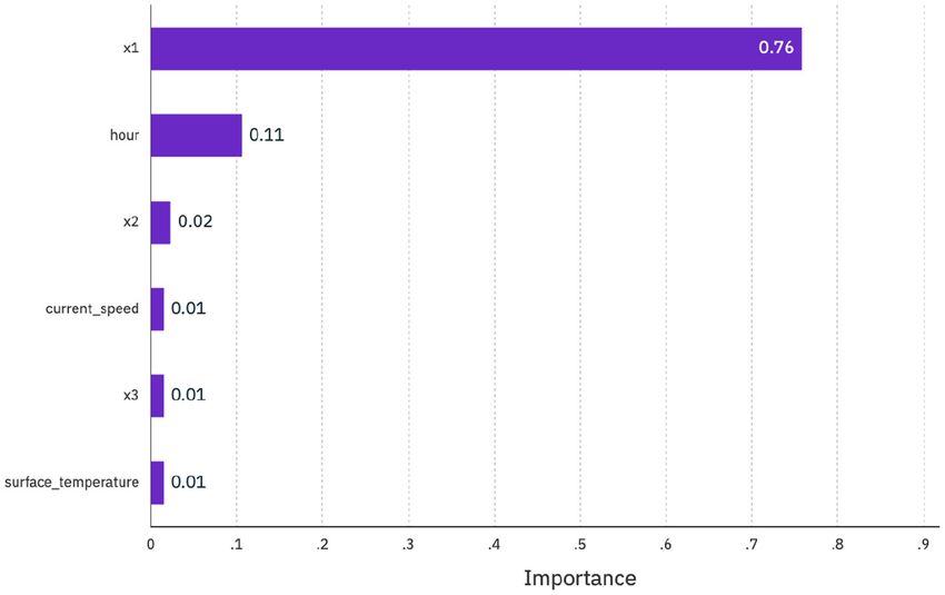
O’Donncha et al.                                                                                                                              Data Driven Aquaculture

TABLE 2 | Synopsis of data collection at the three sites summarising the environmental variables collected and the sampling periods, source of ocean model data (used
to augment sensor data), and weather data source and variables.

                                     NOR                                                   SCO                                        CAN

Environmental sensor                 Aanederaa                                             Realtime Aquaculture                       Realtime Aquaculture
Deployment dates                     21/05/2019–02/10/2019                                 13/11/2019–04/02/2020                      16/09/2019–16/11/2019
Variables                            Temperature, DO, salinity, current speed              Temperature, DO                            Temperature, DO, current speed
Hydroacoustic sensor                 Aquaculture Biomass Monitor                           CageEye                                    CageEye
Deployment dates                     20/02/2019–31/10/2019                                 01/06/2019–29/09/2019                      11/09/2019–30/10/2019
Ocean model data source              NorKyst-800                                           Copernicus Atlantic North West Shelf       Copernicus Global Ocean
Weather data source                                                                   IBM Environmental Intelligence Suite
Weather variables                                                                 Wind speed, air temperature, solar radiation

were depth-averaged to generate a time series vector that is                                 The subset of environmental data were selected based on
amenable toward machine learning analysis. Equation 1 was                                    analysis of literature and the features identified as being
used to compute the mean of grouped data.                                                    important in the first experiment above. This configuration
                                                                                             did not include sliding window values from previous timesteps
                                        P                                                    which simplified the setup (missing data no longer had to be
                                          fx
                                   x̄ = P                                       (1)          interpolated, instead those rows could be simply dropped). It
                                           f
                                                                                             also provides more flexibility when prescribing the prediction
where x refers to the midpoint of depth intervals and f denotes                              window since once could forecast whenever environmental
the frequency of fish in a given interval.                                                   data is available [e.g., one could leverage the Copernicus
    Data gaps or missing values were either imputed or removed:                              10-day ahead ocean forecast data (Tonani et al., 2019) to
if the gap was less than 4 h, data were imputed using a                                      make corresponding 10-day ahead predictions]. The selected
nearest neighbour linear interpolation, while if gaps were greater                           features for this configuration were: temperature, DO, current
than (or equal) 4 h, this portion was removed from analysis                                  speed and direction, wind speed and direction, sea surface
(i.e., both the environmental and hydroacoustic data were                                    height, and hour of day (described in Table 2).
removed). Autoregressive features (i.e., values at previous points
in time) are often informative for machine learning models.                               The features (environmental data primarily) and label (fish
We generated these features using 3 h sliding window size                                 location) data were split into two groups, to form the training-
(i.e., values at previous 1, 2, and 3 h). The resulting matrix                            data set composed of 90% of the data, and the test-data set the
is combined with environmental data, and time-aligned. We                                 remaining 10%. After preprocessing and hourly-averaging, the
used our open-source packages, TSML (Palmes et al., 2020) and                             total number of data points available were 5,847, 1,574, and 840
AutoMLPipeline (Palmes, 2020) for this preprocessing step. The                            data points for the NOR, SCO, and CAN study sites, respectively.
code we used along with the data from the NOR site is available                           The data were provided to the IBM AutoAI tool (IBM,
on Github at (O’Donncha and Palmes, 2021).                                                2021a) which automatically selected the optimal combination of
    As part of the machine learning model setup, we investigated                          algorithm, feature transformations, and calibration parameters
two configurations:                                                                       (or hyperparameters) that minimised prediction error. Mean-
                                                                                          squared-error (MSE) was selected as the loss function to
• All features: all available environmental variables together                            optimise. We then used the trained machine learning model to
  with sliding window values of fish location data were                                   interrogate how environmental data contributed to variations in
  provided to the model. Each row represents the autoregressive                           fish location and behaviour. This can be considered the true goal
  features together with the date-time features (year, month,                             of the machine learning implementation, and an accurate model
  day hour, day of week, etc.), and environmental data. These                             simply served as a means to achieve this goal.
  features are time-aligned with the corresponding label (i.e.,
  fish location) at the desired prediction window. We setup
  the problem as a 1-h ahead prediction using 3 h sliding                                 3. RESULTS
  window size (i.e., autoregressive at previous 3 h were
  included) with 1 h stride. Due to the lack of nighttime                                 We collected data on the observed vertical distribution of relative
  observations we did not implement this analysis at SCO                                  intensity of fish biomass within a cage at three sites. The sites were
  site since the incomplete daily data can reduce the insight                             geographically disparate and had distinct characteristics in terms
  from autoregressive analysis. Instead, at SCO site, we only                             of both the local environment, and the farm itself that influenced
  considered the configuration below.                                                     fish behaviour.
• Selected features: to interrogate the strength of relationship                              Figure 3 presents summary statistics for the NOR site: the
  or dependency between fish location and environmental                                   top figure shows the centrepoint of the fish biomass over the
  conditions, a subset of features were provided to the model.                            duration of the study period, while bottom figure presents a box

Frontiers in Animal Science | www.frontiersin.org                                     7                                           July 2021 | Volume 2 | Article 695054
O’Donncha et al. Data Driven Aquaculture
FIGURE 2 | Data processing workflow outlining the main steps of hydroacoustic data binning, data cleansing, environmental data processing, data merging, and
finally machine learning model implementation.
plot elucidating hourly distribution every month. While each site the time, with the box plot whiskers rarely extending outside this
exhibit unique characteristics, a number of common qualitative range. It’s important to note that due to the CageEye transducer
trends were shared, including: being placed inside the cage (because of the shallow water depth),
some portion of fish in the cage will not be captured by the
• Each site demonstrated diurnal patterns to varying degrees
sensor. Hence, the degree of clustering is likely overestimated
(however the prominence of these varied across sites and at
in this case. Results illustrate that average fish position in the
different times of year).
cage tended to move closer to the surface during the summer
• Observations suggested a weak seasonal-scale pattern,
period, likely influenced by warming surface temperatures.
with fish being at a higher position in the cage during
Figure 5 includes temperature data reported at the Scotland site,
summer months.
illustrating warmer waters that peaked in early August before
• A very pronounced preference for the upper portion of the
returning to moderate temperatures in September. The general
cage that was independent of absolute depth. Generally fish
trend of monthly variations in fish position, seem to follow these
tended to cluster in the upper one-third of the cage which can
patterns, with July and September reporting comparable values
have significant implications for the density of fish in a cage (if
for both temperatures and average fish positions. There was no
the volume of the cage actually used by the fish is far less than
clear diurnal pattern obvious in the data. It is important to note
the volume available).
that due to lack of power during the night, data were not collected
These observations are interrogated in more detail in remainder between the hours of 18:00 and 06:00. This naturally reduced the
of paper. contribution of hour-of-day toward explaining the data.
Figure 3 presents data from the Norwegian farm highlighting Finally, Figure 6 presents data from one of the cages at the
a number of noticeable trends. Firstly, despite the deep waters CAN site. The CageEye sensor was deployed between 11/09/2019
(approximately 60 m), and the large depth of the cage (27 m), and 30/10/2019, covering a period of large drop in temperature
fish tended to congregate in the upper third, and spent most of and reduction in daylight hours. A strong diurnal pattern was
the time at depths of 3–9 m. The box plot does not show any evident at this site with fish tending deeper in the cage during
pronounced daily pattern. It is worth noting that the northerly daylight hours. Due to the time of year the water column was not
latitude of the site (67◦ N) means it is characterised by 24 h thermally stratified which may reduce the effects of temperature.
sunlight for most of the summer months which likely impeded While the cage depth is 10 m, the box plot illustrates that fish
the development of daily patterns during some of the period. were generally clustered within a 2 m range and this cluster rarely
Further, fish in the cage were changed between 26 and 29th July goes deeper than 4 m in the cage, reflecting similar patterns to the
and new stock introduced, which naturally modifies recurrent other two sites.
patterns of behaviour. This may be the source of the more widely Prior to more detailed statistical analysis of the data, one
dispersed patterns of position evident in August, since the fish desires insight into the primary drivers that explains the
were newly introduced to the cage and conceptually displayed observations. As discussed in section 2.3, machine learning
more chaotic behaviour patterns. Moving past these extenuating models such as Random Forest provides a robust approach to
circumstances, the behaviours in September and October are efficiently explore multiple variables and associated response. We
possibly most indicative of typical cage-fish behaviour. These considered an analysis of the CageEye/ABM vertical distribution
months are characterised by a weak diurnal pattern and fish data from the three sites using IBM AutoAI (IBM, 2021a),
congregating toward an ambient depth of about 9 m (or a third automated machine learning tool. The data were preprocessed
of the depth). as described in section 2.3 and uploaded to the AutoAI website.
Figure 4 summarises information on fish distribution at the The hydroacoustic data column was specified as training labels,
Scotland site. Both cage and water depth were significantly and features were selected based on the particular experimental
shallower at this farm, being 6 and 10 m, respectively. Naturally configuration (either “all features” or “selected features”) using
this affects the range that fish could travel and we see a quite tight the AutoAI Graphical User Interface (GUI).
clustering of average fish position between 1 and 2 m. Box plot Our first experimental configuration (“all features” described
indicates that fish sat within a tight half-metre cluster most of in section 2.3) provided a wide range of environmental
Frontiers in Animal Science | www.frontiersin.org 8 July 2021 | Volume 2 | Article 695054O’Donncha et al. Data Driven Aquaculture
FIGURE 3 | Vertical distribution of fish in a cage at NOR farm illustrating the evolution of the centrepoint of fish biomass over the duration of study period (top) and
boxplot of the data grouped into hourly intervals for each month (bottom). The box plot provides insight into distinct patterns developing in the data at different times
with the color legend representing hour of day. Lines extending from the boxplot represent the range of data (i.e., minimum and maximum values), while the box
section reports 25th percentile, median, and 75th percentile values. Filled circles represent outliers for the data.
(temperature, DO, current speed and direction, wind speed and after permuting the feature. A feature is “important” if permuting
direction, and sea surface height), temporal (hour of day, day of its values increases the model error, because the model relied
year), and autoregressive (measured fish position at 1, 2, and 3 on the feature for the prediction. A feature is “unimportant” if
h previously) variables as input (or features) to the model. The permuting its values keeps the model error unchanged, because
model was trained to make a 1-h-ahead prediction. Since the the model ignored the feature for the prediction (Breiman, 2001).
model implicitly learned to predict by learning the relationship Data from the CAN site provided some useful insight into
between features and labels, we could then use the trained model salmon cage dynamics. As might be expected, autoregressive
to extract insight on how these features contributed to the model variables were a primary driver of fish behaviour. The most
prediction. The resultant model demonstrate strong predictive important feature is value at the previous timestamp (x1,
skill reporting explained variance of 76, 81, and 75% for the NOR, denoting fish position 1 h previously) with x2 and x3 also
SCO, and CAN sites, respectively. The relatively high correlation contributing. Hour-of-day was the second most important
scores (equalling 0.87, 0.9, and 0.87, respectively) support the feature which suggests that there was some diurnal pattern
viability of using the model to explore the contribution that to the data that can be explained by this repeating feature.
individual variables or features make toward prediction. This information can serve to guide optimal feature selection
Figure 7 presents the feature importance of the supplied for model development. Combined with domain knowledge on
data to the response variable or model prediction at the CAN primary variables that influence fish behaviour (summarised
site (extracted from the AutoAI GUI). The feature importance in section 1.2), this information can lead to development of
measure computes the contribution or importance of each a more effective model. Selecting the most appropriate set of
feature by calculating the increase of the model’s prediction error features is critical to maximising model performance, while from
Frontiers in Animal Science | www.frontiersin.org 9 July 2021 | Volume 2 | Article 695054O’Donncha et al. Data Driven Aquaculture
FIGURE 4 | Vertical distribution of fish in a cage at SCO farm illustrating the evolution of the centrepoint of fish biomass over the duration of study period (top) and
boxplot of the data grouped into hourly intervals for each month (bottom). The box plot provides insight into distinct patterns developing in the data at different times
with the color legend representing hour of day.Lines extending from the boxplot represent the range of data (i.e., minimum and maximum values), while the box section
reports 25th percentile, median, and 75th percentile values. Filled circles represent outliers for the data. Note that the plots only include data between 06:00 and 18:00.
a practical point of view a model with less predictors may be more of the signal. In particular, trends in the data are adequately
interpretable (Kuhn and Johnson, 2013). tracked and the model accurately replicates whether the fish
Our second experimental setup involved a reduced set of move up or down in the cage in response to the provided
features, namely: temperature, DO, current speed, wind speed, model inputs. From a feature analysis perspective, this allows
and salinity, together with hour-of-day. Choice of features were us to confidently interrogate results since we are primarily
based on both feature importance reported in Figure 7 and those interested in variations in output rather than magnitude (i.e.,
suggested by literature. Naturally, the variance explained (or changes of fish position in response to changes in environmental
predictive skill) of the model dropped with the reduced feature conditions rather than the magnitude of those changes) We used
set, but the analysis of feature importance or contributions can be the model to understand variance explained by these drivers
more meaningful. The resultant model explained 59%, 64%, and together with the feature importance of each. Figure 9 presents
61% of variance for the NOR, SCO, and CAN sites, respectively, the variable importance computed for the three locations in
which represents a drop of 14–17% compared to the model with Norway, Scotland, and Canada.
all features provided. This drop in predictive skill was balanced While there were similarities in the drivers that influenced
by an improvement in model interpretability and increased focus fish position at the three sites, pronounced variations existed
on pertinent variables (environmental conditions). based on the different geography and characteristics of each site.
Figure 8 summarises model performance at the Canada site. It As suggested by both feature importance analysis and boxplot
illustrates that the model captures data trends quite well reporting visualisation, time-of-day was a primary driver, particularly at the
correlation score of 0.78. Visually, the model captures observed Canadian farm. This reflected the pronounced diurnal patterns
fish depth quite well considering the highly dynamic nature that are visually evident in Figures 3–6, with the fish being
Frontiers in Animal Science | www.frontiersin.org 10 July 2021 | Volume 2 | Article 695054O’Donncha et al. Data Driven Aquaculture
FIGURE 5 | Time series plot of temperature (top row), and DO (bottom row) reported at the three sites, NOR (left), SCO (middle), and CAN (right), respectively.
deeper in cage during daylight hours. It’s worth noting that at the NOR site which illustrates both fish sensitivities and
diurnal patterns were likely under represented in NOR and local bay characteristics.
SCO data due to long summertime daylight hours and lack Figure 11 presents vertical profile of temperature and salinity
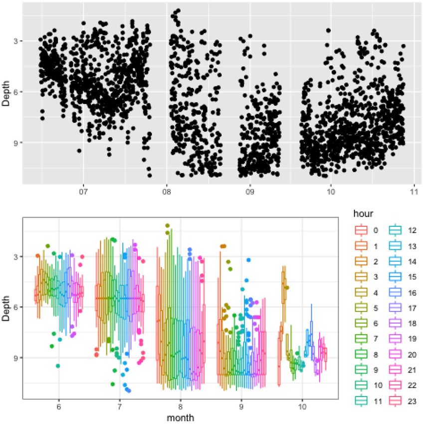
of nighttime observations, respectively. Figure 10 presents a at the site over the duration of the study period. Results illustrate
density plot of daytime and nighttime fish positions for both a pronounced thermal stratification during the summer months,
CAN and NOR (due to lack of nighttime observations, SCO that breaks down into a well-mixed water column in spring
was excluded). To remove the effects of long sunshine hours and autumn. Variations of vertical salinity are more complex
during June and July in NOR these 2 months were excluded illustrating relatively low surface salinity values in September,
from the plot. Results demonstrated a clear difference between which may be influenced by precipitation or freshwater runoff.
daytime and nighttime behaviour for the CAN site and a similar Literature indicates that Atlantic salmon are influenced by
but much less pronounced difference for the NOR site. In salinity variations when younger than 3 months and during
Canada, fish congregated at about 3.6 m depth and the spread spawning periods, while indifferent to salinity at other times
around this was quite narrow during the day, while at night, (Oppedal et al., 2011). The behavioural influence detected in this
fish were distributed more widely across the water column study may be a result of salmon expressing preference for lower
with a mean depth of 2.8 m. Similar trends were observed in salinity waters in spring, during the return migration period of
Norway (although not as pronounced). The mean difference salmon toward freshwater. However, Figure 11 indicates that the
between daytime and nighttime positions were 0.52 m while vertical variation in salinity was relatively small, and additional
fish were also more uniformly spread across the water column study is necessary to understand the influence this may have on
at night. salmon variations.
At all sites, physical oceanographic variables represented an While Figures 7, 9 provide insight into which features were
important driver. Physical mixing by current speeds and wind important, we were interested in how the features influence
forcing were particularly critical at the CAN site and three of the the predicted outcome. A powerful approach to interrogate
five most important variables represented physical stresses and the variations of predictand in response to predictors are
mechanical mixing, namely current direction, wind direction, accumulated local effects (ALE) (Apley and Zhu, 2020). ALE
and wind speed, respectively (in order of influence). Wind stress quantifies the contributions of different predictors by considering
did not represent an important driver of fish depth variance at the conditional probability or likelihood of changes to prediction.
the NOR site. This is likely due to the increased depth of cage It has noted advantages in cases where multiple predictors are
and fish position serving to shelter from local surface dynamics. correlated and the effects are difficult to separate (which is
Interestingly, salinity was the primary driver of fish position naturally the case in ocean systems).
Frontiers in Animal Science | www.frontiersin.org 11 July 2021 | Volume 2 | Article 695054O’Donncha et al. Data Driven Aquaculture
FIGURE 6 | Vertical distribution of fish in a cage at CAN farm illustrating the evolution of the centrepoint of fish biomass over the duration of study period (top) and
boxplot of the data grouped into hourly intervals for each month (bottom). The box plot provides insight into distinct patterns developing in the data at different times
with the colour legend representing hour of day. Lines extending from the boxplot represent the range of data (i.e., minimum and maximum values), while the box
section reports 25th percentile, median, and 75th percentile values. Filled circles represent outliers for the data.
Figure 12 presents the computed ALE for the CAN site for The contribution of wind and current speed to fish response
four variables, namely, temperature, DO, wind, and current speed were quite similar (as might be expected). Generally increased
to the response variable. ALE provides a quantitative way to current speed invoked an increase in the model predicted value
show how the prediction (fish position) changes locally, when the (i.e., fish were deeper in the cage). The plot suggests a linear
feature (environmental variable) is varied. The marks on the x- relationship but is likely not enough data to draw confident
axis indicates the distribution of the particular feature, showing conclusions on the exact relationship. This is amplified by the fact
how relevant a region is for interpretation (little or no points that the marks on the x-axis are quite sparse for higher values of
mean that we should not over-interpret this region). Figure 12 wind and current speed indicating low number of observations
allows for extraction of a number of pertinent observations for these conditions.
on the data. The feature effects of temperature and oxygen
suggest that “ambient” conditions had low importance (tends
4. DISCUSSION AND CONCLUSIONS
toward zero), while higher and lower values tends to trigger a
response. Specifically, DO reports low importance when values The precision aquaculture concept aims to exploit data-driven
were between 7–8 mgL−1 , while values outside this range invoke management of fish production, thereby improving the farmer’s
a large response by the model. It is worth noting that this ability to monitor, control and document biological processes in
large response by the fish is likely indicative of high-stress fish farms. The fundamental approach has been summarised as
conditions. Figure 5 plots time series of DO to illustrate the a series of steps, namely observe, interpret, decide, and act (Føre
evolution at the site and localised periods when values dropped et al., 2018), that strives toward optimised operations of farms.
below 7 mgL−1 . Where precision aquaculture differs most prominently from its
Frontiers in Animal Science | www.frontiersin.org 12 July 2021 | Volume 2 | Article 695054You can also read