Image Aesthetic Assessment: An Experimental Survey - arXiv.org

1

 Image Aesthetic Assessment:
 An Experimental Survey
 Yubin Deng, Chen Change Loy, Member, IEEE, and Xiaoou Tang, Fellow, IEEE

 Abstract—This survey aims at reviewing recent computer vision techniques used in the assessment of image aesthetic quality. Image
 aesthetic assessment aims at computationally distinguishing high-quality photos from low-quality ones based on photographic rules,
 typically in the form of binary classification or quality scoring. A variety of approaches has been proposed in the literature trying to solve
 this challenging problem. In this survey, we present a systematic listing of the reviewed approaches based on visual feature types
 (hand-crafted features and deep features) and evaluation criteria (dataset characteristics and evaluation metrics). Main contributions
 and novelties of the reviewed approaches are highlighted and discussed. In addition, following the emergence of deep learning
arXiv:1610.00838v2 [cs.CV] 20 Apr 2017

 techniques, we systematically evaluate recent deep learning settings that are useful for developing a robust deep model for aesthetic
 scoring. Experiments are conducted using simple yet solid baselines that are competitive with the current state-of-the-arts. Moreover,
 we discuss the possibility of manipulating the aesthetics of images through computational approaches. We hope that our survey could
 serve as a comprehensive reference source for future research on the study of image aesthetic assessment.

 Index Terms—Aesthetic quality classification, image aesthetics manipulations

 F

 1 I NTRODUCTION

 T HE aesthetic quality of an image is judged by com-
 monly established photographic rules, which can be
 affected by numerous factors including the different usages
 As the volume of visual data available online grows at an
 exponential rate, the capability of automatically distinguish-
 ing high-quality images from low-quality ones gain increas-
 of lighting [1], contrast [2], and image composition [3] (see ing demands in real-world image searching and retrieving
 Fig. 1a). These human judgments given in an aesthetic eval- applications. In image search engines, it is expected that
 uation setting are the results of human aesthetic experience, the systems will return professional photographs instead
 i.e., the interaction between emotional-valuation, sensory- of random snapshots when a particular keyword is en-
 motor, and meaning-knowledge neural systems, as demon- tered. For example, when a user enters “mountain scenery”,
 strated in a systematic neuroscience study by Chatterjee et he/she will expect to see colorful, pleasing mountain views
 al. [4]. From the beginning of psychological aesthetics stud- or well-captured mountain peaks instead of gray or blurry
 ies by Fechner [5] to modern neuroaesthetics, researchers mountain snapshots.
 argue that there is a certain connection between human The design of these intelligent systems can potentially
 aesthetic experience and the sensation caused by visual be facilitated by insights from neuroscience studies, which
 stimuli regardless of source, culture, and experience [6], show that human aesthetic experience is a kind of informa-
 which is supported by activations in specific regions of tion processing that includes five stages: perception, implicit
 the visual cortex [7], [8], [9], [10]. For example, human’s memory integration, explicit classification of content and
 general reward circuitry produces pleasure when people style, cognitive mastering and evaluation, and ultimately
 look at beautiful objects [11], and the subsequent aesthetic produces aesthetic judgment and aesthetic emotion [12],
 judgment consists of the appraisal of the valence of such [13]. However, it is non-trivial to computationally model
 perceived objects [8], [9], [10], [12]. These activations in this process. Challenges in the task of judging the quality
 the visual cortex can be attributed to the processing of of an image include (i) computationally modeling the inter-
 various early, intermediate and late visual features of the twined photographic rules, (ii) knowing the aesthetical dif-
 stimuli including orientation, shape, color grouping and ferences in images from different image genres (e.g., close-
 categorization [13], [14], [15], [16]. Artists intentionally in- shot object, profile, scenery, night scenes), (iii) knowing the
 corporate such features to facilitate desired perceptual and type of techniques used in photo capturing (e.g., HDR,
 emotional effects in viewers, forming a set of guidelines black-and-white, depth-of-field), and (iv) obtaining a large
 as they create artworks to induce desired responses in amount of human-annotated data for robust testing.
 the nervous systems of perceivers [16], [17]. And modern To address these challenges, computer vision researchers
 day photographers now resort to certain well-established typically cast this problem as a classification or regression
 photographic rules [18], [19] when they capture images as problem. Early studies started with distinguishing typi-
 well, in order to make their work appealing to a large group cal snapshots from professional photographs by trying to
 of audiences. model the well-established photographic rules using low-
 level features [20], [21], [22]. These systems typically in-
 • Y. Deng, C. C. Loy and X. Tang are with the Department of Information volve a training set and a testing set consisting of high-
 Engineering, The Chinese University of Hong Kong. quality images and low-quality ones. The system robustness
 E-mail: {dy015, ccloy, xtang}@ie.cuhk.edu.hk
 is judged by the model performance on the testing set

2

 Input Image

 Feature Extraction

 Handcrafted Features Deep Features

 Simple image features Generic deep features
 Generic features Learned aesthetic deep
 Non-generic features features
 Component 1

 Decision Phase

 Classification Regression

 Naive Bayes Linear Regressor
 Support Vector Machine Support Vector Regressor
 Deep Neural Network Customized Regressor
 Component 2
 (a) Row 1: Color harmony. (b)
 Row 2: Single salient object and low depth-of-field. Binary Label / Aesthetic Score
 Row 3: Black-and-white portraits with decent lighting contrast.
Fig. 1. (a) High-quality images following well-established photographic rules. (b) A typical flow of image aesthetic assessment systems.

using a specified metric such as accuracy. These rule-based methodologies. Specifically, as different datasets exist and
approaches are intuitive as they try to explicitly model the evaluation criteria vary in the image aesthetics literature, we
criteria that humans use in evaluating the aesthetic quality do not aim at directly comparing the system performance
of an image. However, more recent studies [23], [24], [25], of all reviewed work; instead, in the survey we point out
[26] have shown that using a data-driven approach is more their main contributions and novelties in model designs,
effective, as the amount of training data available grows and give potential insights for future directions in this field
from a couple of hundreds of images to millions of images. of study. In addition, following the recent emergence of
Besides, transfer learning from source tasks with sufficient deep learning techniques and the effectiveness of the data-
amount of data to a target task with relatively fewer training driven approach in learning better image representations,
data is also proven feasible, with many successful attempts we systematically evaluate different techniques that could
showing promising results by deep learning methods [27] facilitate the learning of a robust deep classifier for aesthetic
with network fine-tune, where image aesthetics are implic- scoring. Our study covers topics including data preparation,
itly learned in a data-driven manner. fine-tune strategies, and multi-column deep architectures,
 As summarized in Fig. 1b, the majority of aforemen- which we believe to be useful for researchers working in
tioned computer vision approaches for image aesthetic as- this domain. In particular, we summarize useful insights
sessment can be categorized based on image representa- on how to alleviate the potential problem of data distri-
tions (e.g., handcrafted features and learned features) and bution bias in a binary classification setting and show the
classifiers/regressors training (e.g., Support Vector Machine effectiveness of rejecting false positive predictions using our
(SVM) and neural network learning approaches). To our proposed convolution neural network (CNN) baselines, as
best knowledge, there does not exist up-to-date survey that revealed by the balanced accuracy metric. Moreover, we also
covers the state-of-the-art methodologies involved in image review the most commonly used publicly available image
aesthetic assessment. The last review was published in 2011 aesthetic assessment datasets for this problem and draw
by Joshi et al. [28], and no deep learning based methods connections between image aesthetic assessment and image
were covered. Some reviews on image quality assessment aesthetic manipulation, including image enhancement, com-
have been published [29], [30]. In those lines of effort, image putational photography and automatic image cropping. We
quality metrics regarding the differences between a noise- hope that this survey can serve as a comprehensive refer-
tempered sample and the original high-quality image have ence source and inspire future research in understanding
been proposed, including but not limited to mean squared image aesthetics and its many potential applications.
error (MSE), structural similarity index (SSIM) [31] and
visual information fidelity (VIF) [32]. Nevertheless, their 1.1 Organization
main focus is on distinguishing noisy images from clean The rest of this paper is organized as follows. We first give
images in terms of a different quality measure, rather than a review of deep neural network basics and recap the objec-
artistic/photographic aesthetics. tive image quality metrics in section 2. Then in Section 3,
 In this article, we wish to contribute a thorough we explain the typical pipeline used by the majority of
overview of the field of image aesthetic assessment; mean- the reviewed work on this problem and highlight the most
while, we will also cover the basics of deep learning concerned design component. We review existing datasets

3

in Section 4. We present a review on conventional methods Reference Gaussian blur, σ = 1 Gaussian blur, σ = 2
 PSNR / SSIM / VIF 26.19 / 0.86 / 0.48 22.71 / 0.72 / 0.22
based on handcrafted features in Section 5 and deep features
in Section 6. Evaluation criteria and existing results are dis-
cussed in Section 7. In Section 8, we systematically analyze
various deep learning settings using a baseline model that is
competitive with the state-of-the-arts. In Section 9, we draw
a connection between aesthetic assessment and aesthetic
manipulation, with a focus on aesthetic-based image crop-
ping. Finally, we conclude with a discussion of the current
state of research and give some recommendations for future Reference High-quality Image Low-quality Image
 PSNR / SSIM / VIF 7.69 / -0.13 / 0.04 8.50 / 0.12 / 0.03
directions on this field of study.

2 BACKGROUND
2.1 Deep Neural Network
Deep neural network belongs to the family of deep learning
methods that are tasked to learn feature representation in
a data-driven approach. While shallow models (e.g., SVM,
boosting) have shown success in earlier literatures concern-
ing relatively smaller amounts of data, they require highly- Fig. 2. Quality measurement by Peak Signal-to-Noise Ratio (PSNR),
 Structural Similarity Index (SSIM) [31] and Visual Information Fidelity
engineered feature designs in solving machine learning (VIF) [32] (higher is better, typically measured against a referencing
problems. Common architectures in deep neural networks groundtruth high-quality image). Although these are good indicators for
consist of a stack of parameterized individual modules measuring the quality of images in image restoration applications as in
 Row 1, they do not reflect human perceived aesthetic values as shown
that we call “layers”, such as convolution layer and fully- by the measurements for the building images in Row 2.
connected layer. The architecture design of stacking layers
on top of layers is inspired by the hierarchy in human
visual cortex ventral pathway, offering different levels of where η is the learning rate. In our example, ∆W can be
abstraction for the learned representation in each layer. In- easily derived based on the chain rule:
formation propagation among layers in feed-forward deep
neural networks typically follows a sequential manner. A ∂L
 ∆W =
“forward” operation F (·) is defined respectively in each ∂W
layer to propagate the input x it receives and produces ∂L ∂z ∂y
 = (4)
an output y to the next layer. For example, the forward ∂z ∂y ∂W
operation in a fully-connected layer with learnable weights exp(−y)
W can be written as: = (z − t) · ·x
 (exp(−y) + 1)2
 X
 y = F (x) = Wx = wij · xi (1) In practice, researchers resort to batch stochastic gradient
 descent (SGD) or more advanced learning procedures that
This is typically followed by a non-linear function, such as
 compute more stable gradients as averaged from a batch of
sigmoid
 training examples {(xi , ti )|xi ∈ X} in order to train deeper
 1
 z= (2) and deeper neural networks with continually increasing
 1 + exp(−y) amounts of layers. We refer readers to [27] for an in-depth
or the rectified linear unit (ReLU) z = max(0, y), which acts overview of more deep learning methodologies.
as the activation function and produces the net activation
output z .
 2.2 Image Quality Metrics
 To learn the weights W in a data-driven manner, we
need to have the feedback information that reports the Image quality metrics are defined in an attempt to quan-
current performance of the network. Essentially, we are titatively measure the objective quality of an image. This
trying to tune the knobs W in order to achieve a learning is typically used in image restoration applications (super-
objective. For example, given an objective t for the input resolution [34], de-blur [35] and de-artifacts [36]) where we
x, we want to minimize the squared error between the net have a default high-quality reference image for comparison.
output z and t by defining a loss function L: However, these quality metrics are not designed to measure
 the subjective nature of human perceived aesthetic quality
 1
 L= ||z − t||2 (3) (see examples in Fig. 2). Directly applying these objective
 2 quality metrics to our concerned domain of image aesthetic
To propagate this feedback information to the weights, we assessment may produce misleading results, as can be seen
define the “backward” operation for each layer using the from the measured values in the second row of Fig. 2. Devel-
gradient back-propagation [33]. We hope to get the direction oping more robust metrics has gained increasing interests in
∆W to update the weights W in order to better suit the the research community in an attempt to assess the more
training objective (i.e., to minimize L): W ← W − η∆W, subjective image aesthetic quality.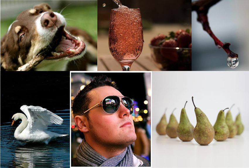

4

3 A T YPICAL P IPELINE The Photo.Net dataset and The DPChallenge dataset
Most existing image quality assessment methods take a are introduced in [28], [60]. These two datasets can be con-
supervised learning approach. A typical pipeline assumes sidered as the earliest attempt to construct large-scale image
a set of training data {xi , yi }i∈[1,N ] , from which a function database for image aesthetic assessment. The Photo.Net
f : g(X) → Y is learned, where g(xi ) denotes the feature dataset contains 20,278 images with at least 10 score ratings
representation of image xi . The label yi is either {0, 1} for per image. The rating ranges from 0 to 7 with 7 assigned
binary classification (when f is a classifier) or a continuous to the most aesthetically pleasing photos. Typically, images
score range for regression (when f is a regressor). Following uploaded to Photo.net are rated as somewhat pleasing, with
this formulation, a pipeline can be broken into two main the peak of the global mean score skewing to the right in
components as shown in Fig. 1b, i.e., a feature extraction the distribution [28]. The more challenging DPChallenge
component and a decision component. dataset contains diverse rating. The DPChallenge dataset
 contains 16,509 images in total, and has been later replaced
 by the AVA dataset, where a significantly larger amount
3.1 Feature Extraction
 of images derived from DPChallenge.com are collected and
The first component of an image aesthetics assessment annotated.
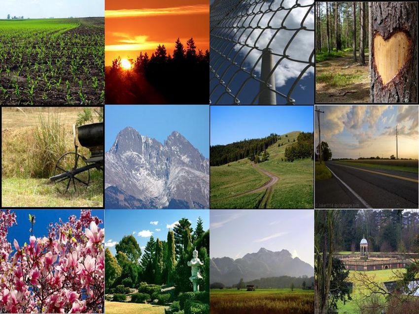
system aims at extracting robust feature representations The CUHK-PhotoQuality (CUHK-PQ) dataset is intro-
describing the aesthetic aspect of an image. Such features duced in [45], [61]. It contains 17,690 images collected from
are assumed to model the photographic/artistic aspect of DPChallenge.com and amateur photographers. All images
images in order to distinguish images of different qualities. are given binary aesthetic label and grouped into 7 scene
Numerous efforts have been seen in designing features that categories, i.e., “animal”, “plant”, “static”, “architecture”,
are robust enough for the intertwined aesthetic rules. The “landscape”, “human”, and “night”. The standard training
majority of feature types can be classified into handcrafted and testing set from this dataset are random partitions of
features and deep features. Conventional approaches [20], 50-50 split or a 5-fold cross validation partition, where the
[21], [37], [38], [39], [40], [41], [42], [43], [44], [45], [46], [47], overall ratio of the total number of positive examples and
[48], [49] typically adopt handcrafted features to computa- that of the negative examples is around 1 : 3. Sample images
tionally model the photographic rules (lighting, contrast), are shown in Fig. 3.
global image layout (rule-of-thirds) and typical objects (hu- The Aesthetic Visual Analysis (AVA) dataset [49] con-
man profiles, animals, plants) in images. In more recent tains ∼ 250k images in total. These images are obtained
work, generic deep features [50], [51] and learned deep from DPChallenge.com and labeled by aesthetic scores.
features [23], [24], [25], [52], [53], [54], [55], [56], [57], [58], Specifically, each image receives 78 ∼ 549 votes of score
[59] exhibit stronger representation power for this task. ranging from 1 to 10. The average score of an image is
 commonly taken to be its groundtruth label. As such, it
3.2 Decision Phase contains more challenging examples as images lie within
The second component of an image aesthetics assessment the center score range could be ambiguous in their aesthetic
system provides the ability to perform classification or re- aspect (Fig. 4a). For the task of binary aesthetic quality
gression for the given aesthetic task. Naı̈ve Bayes classifier, classification, images with an average score higher than
SVM, boosting and deep classifier are typically used for threshold 5 + σ are treated as positive examples, and images
binary classification of high-quality and low-quality images, with an average score lower than 5 − σ are treated as neg-
whereas regressors like support vector regressor are used in ative ones. Additionally, the AVA dataset contains 14 style
ranking or scoring images based on their aesthetic quality. attributes and more than 60 category attributes for a subset
 of images. There are two typical training and testing splits
 from this dataset, i.e., (i) a large-scale standardized partition
4 DATASETS with ∼ 230k training images and ∼ 20k testing images
The assessment of image aesthetic quality assumes a stan- using a hard threshold σ = 0 (ii) and an easier partition
dard training set and testing set containing high-quality modeling that of CUHK-PQ by taking those images whose
image examples and low-quality ones, as mentioned above. score ranking is at top 10% and bottom 10%, resulting in
Judging the groundtruth aesthetic quality of a given image ∼ 25k images for training and ∼ 25k images for testing.
is, however, a subjective task. As such, it is inherently The ratio of the total number of positive examples and that
challenging to obtain a large amount of such annotated of the negative examples is around 12 : 5.
data. Most of the earlier papers [21], [38], [39] on image Apart from these two standard benchmarks, more recent
aesthetic assessment collect a small amount of private image research also introduce new datasets that take into consider-
data. These datasets typically contain from a few hundred ation the data-balancing issue. The Image Aesthetic Dataset
to a few thousand images with binary labels or aesthetic (IAD) introduced in [55] contains 1.5 million images derived
scoring for each image. Yet, such datasets where the model from DPChallenge and PHOTO.NET. Similar to AVA, im-
performance is evaluated are not publicly available. Much ages in the IAD dataset are scored by annotators. Positive
research effort has later been made to contribute publicly examples are selected from those images with a mean score
available image aesthetic datasets of larger scales for more larger than a threshold. All IAD images are used for model
standardized evaluation of model performance. In the fol- training, and the model performance is evaluated on AVA
lowing, we introduce those datasets that are most frequently in [55]. The ratio of the number of positive examples and
used in performance benchmarking for image aesthetic as- that is the negative examples is around 1.07 : 1. The Aes-
sessment. thetic and Attributes DataBase (AADB) [25] also contains a

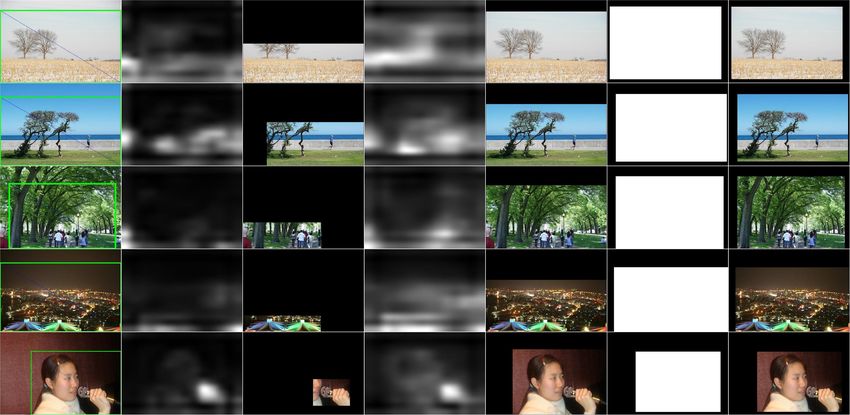
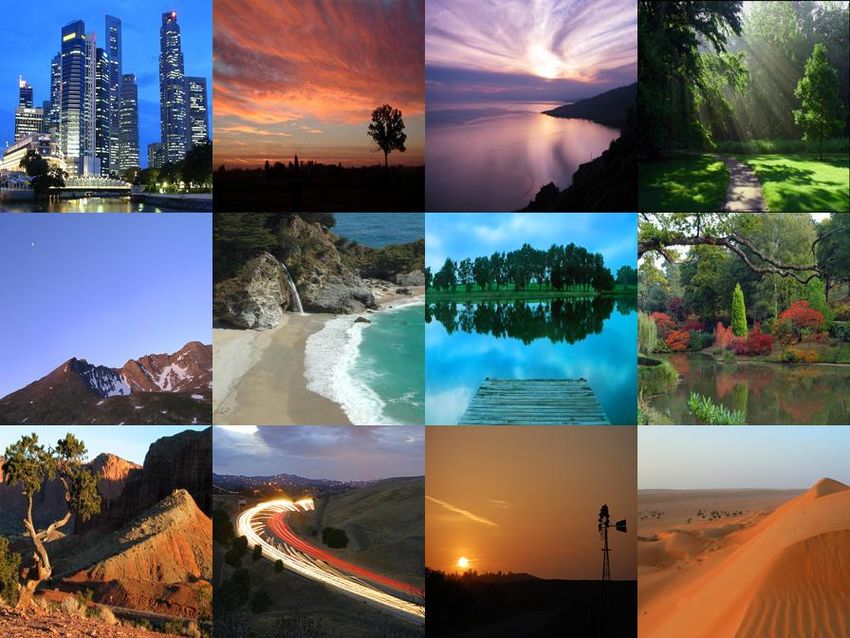
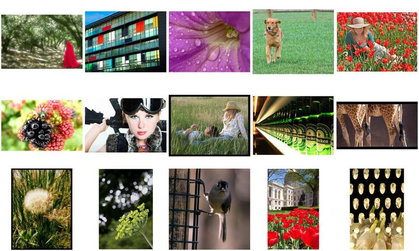
5

 ~4.5k ~13k

 CUHK-PQ Dataset
 # Positive Images
 # Negative Images

 (a) (b)
Fig. 3. (a) Sample images in the CUHK-PQ dataset. Distinctive differences can be visually observed between the high-quality images (grouped in
green) and low-quality ones (grouped in red). (b) Number of images in CUHK-PQ dataset.

 ~160k

 ~70k

 AVA training partition

 ~16k

 ~4k

 AVA testing partition
 # Positive Images
 # Negative Images
 (a) (b)
Fig. 4. (a) Sample images in the AVA dataset. Top: images labeled with mean score > 5, grouped in green. Bottom: images labeled with mean
score < 5, grouped in red. The image groups on the right are ambiguous ones having a somewhat neutral scoring around 5. (b) Number of images
in AVA dataset.

balanced distribution of professional and consumer photos, 5 C ONVENTIONAL A PPROACHES WITH H AND -
with a total of 10, 000 images. Eleven aesthetic attributes CRAFTED F EATURES
and annotators’ ID is provided. A standard partition with
 The conventional option for image quality assessment is to
8,500 images for training, 500 images for validation, and
 hand design good feature extractors, which requires a con-
1,000 images for testing is proposed [25].
 siderable amount of engineering skill and domain expertise.
 The trend to creating datasets of even larger volumes
 Below we review a variety of approaches that exploit hand-
and higher diversity is essential for boosting the research
 engineered features.
progress in this field of study. To date, the AVA dataset
serves as a canonical benchmark for performance evaluation
of image aesthetic assessment as it is the first large-scale 5.1 Simple Image Features
dataset with detailed annotation. Still, the distribution of Global features are first explored by researchers to model the
positive examples and negative ones in the dataset also aesthetic aspect of images. The work by Datta et al. [21] and
play a role in the effectiveness of trained models, as false Ke et al. [37] are among the first to cast aesthetic understand-
positive predictions are as harmful as having low recall rate ing of images into a binary classification problem. Datta et
in image retrieval/searching applications. In the following, al. [21] combine low-level features and high-level features
we review major attempts in the literature to build systems that are typically used for image retrieval and train an SVM
for the challenging task of image aesthetic assessment. classifier for binary classification of images aesthetic quality.

6

 objects and the background scene, then a support vector
 regressor is trained. Wu et al. [65] propose the use of Gabor
 filter responses to estimate the position of the main object
 in images, and extract low-level HSV-color features from
 global and central image regions. These features are fed to
 a soft-SVM classifier with sigmoidal softening in order to
 distinguish images of ambiguous quality. Dhar et al. [44]
 cast high-level features into describable attributes of compo-
Fig. 5. Left: Image composition with low depth-of-field, single salient sition, content and sky illumination and combine low-level
object, and rule-of-thirds. Right: Image of low aesthetic quality.
 features to train an SVM classifier. Lo et al. [66] propose
 the combination of layout composition, edge composition
Ke et al. [37] propose global edge distribution, color dis- features with HSV color palette, HSV counts and global
tribution, hue count and low-level contrast and brightness features (textures, blur, dark channel, contrasts). SVM is
indicators to represent an image, then they train a Naı̈ve used as the classifier.
Bayes classifier based on such features. An even earlier The representative work by Tang et al. [45] give a com-
attempt by Tong et al. [20] adopt boosting to combine global prehensive analysis of the fusion of global features and re-
low-level simple features (blurriness, contrast, colorfulness, gional features. Specifically, image composition is estimated
and saliency) in order to classify professional photograph by global hue composition and scene composition, and
and ordinary snapshots. All these pioneering works present multiple types of regional features extracted from subject
the very first attempts to computationally modeling the areas are proposed, such as dark channel feature, clarity
global aesthetic aspect of images using handcrafted features. contrast, lighting contrast, composition geometry of the sub-
Even in a recent work, Aydın et al. [62] construct image ject region, spatial complexity and human-based features.
aesthetic attributes by sharpness, depth, clarity, tone, and An SVM classifier is trained on each of the features for
colorfulness. An overall aesthetics rating score is heuris- comparison and the final model performance is substan-
tically computed based on these five attributes. Improv- tially enhanced by combining all the proposed features. It
ing upon these global features, later studies adopt global is shown that regional features can effectively complement
saliency to estimate aesthetic attention distribution. Sun et global features in modeling the images aesthetics.
al. [38] make use of global saliency map to estimate visual A more recent approach by image composition features
attention distribution to describe an image, and they train a is proposed by Zhang et al. [67] where image descriptors
regressor to output the quality score of an image based on that characterize local and global structural aesthetics from
the rate of focused attention region in the saliency map. You multiple visual channels are designed. Spatial structure of
et al. [39] derive similar attention features based on global the image local regions are modeled using graphlets, and
saliency map and incorporate temporal activity feature for they are connected based on atomic region adjacency. To
video quality assessment. describe such atomic regions, visual features from multiple
 Regional image features [40], [41], [42] later prove to visual channels (such as color moment, HOG, saliency his-
be effective in complementing the global features. Luo et togram) are used. The global spatial layout of the photo are
al. [40] extract regional clarity contrast, lighting, simplicity, also embedded into graphlets using a Grassmann manifold.
composition geometry, and color harmony features based The importances of the two kinds of graphlet descriptors are
on the subject region of an image. Wong et al. [63] compute dynamically adjusted, capturing the spatial composition of
exposure, sharpness and texture features on salient regions an image from multiple visual channels. The final aesthetic
and global image, as well as features depicting the subject- prediction of an image is generated by a probabilistic model
background relationship of an image. Nishiyama et al [41] using the post-embedding graphlets.
extract bags-of-color-patterns from local image regions with
a grid-sampling technique. While [40], [41], [63] adopt the
SVM classifier, Lo et al. [42] build a statistic modeling system 5.3 General-Purpose Features
with coupled spatial relations after extracting color and
texture feature from images, where a likelihood evaluation Yeh et al. [46] make use of SIFT descriptors and propose
is used for aesthetic quality prediction. These methods focus relative features by matching a query photo to photos in a
on modeling image aesthetics from local image regions that gallery group. General-purpose imagery features like Bag-
are potentially most attracted to humans. of-Visual-Words (BOV) [68] and Fisher Vector (FV) [69]
 are explored in [47], [48], [49]. Specifically, SIFT and color
 descriptors are used as the local descriptors upon which a
5.2 Image Composition Features Gaussian Mixture Model (GMM) is trained. The statistics
Image composition in a photograph typically relates to the up to the second order of this GMM distribution is then
presence and position of a salient object. Rule-of-thirds, encoded using BOV or FV. Spatial pyramid is also adopted
low depth-of-field, and opposing colors are the common and the per-region encoded FV’s are concatenated as the
techniques for composing a good image where the salient final image representation. These methods [47], [48], [49]
object is made outstanding (see Fig. 5). To model such aes- represent the attempt to implicitly modeling photographic
thetic aspect, Bhattacharya et al. [43], [64] propose composi- rules by encoding them in generic content based features,
tional features using relative foreground position and visual which is competitive or even outperforms the simple hand-
weight ratio to model the relations between foreground crafted features.

7

5.4 Task-Specific Features fully-connected
 convolution

Task-specific features refer to features in image aesthetic
assessment that are optimized for a specific category of output
photos, which can be efficient when the use-case or task
scenario is fixed or known beforehand. Explicit information
(such as human face characteristics, geometry tag, scene Fig. 6. The architecture of typical single-column CNNs.
information, intrinsic character component properties) is
exploited based on the different task nature. convolution
 fully-connected

 Li et al. [70] propose a regression model that targets
only consumer photos with faces. Face-related social fea-
tures (such as face expression features, face pose features,
relative face position features) and perceptual features (face output
distribution symmetry, face composition, pose consistency)
are specifically designed for measuring the quality of images
with faces, and it is shown in [70] that they complement
with conventional handcrafted features (brightness contrast,
color correlation, clarity contrast and background color sim- Fig. 7. Typical multi-column CNN: a two-column architecture is shown
plicity) for this task. Support vector regression is used to as an example.
produce aesthetic scores for images.
 Lienhard et al. [71] study particular face features for eval-
uating the aesthetic quality of headshot images. To design component layout features while modeling the aesthetics of
features for face/headshots, the input image is divided into handwritten characters. A back-propagation neural network
sub-regions (eyes region, mouth region, global face region is trained as the regressor to produce an aesthetic score for
and entire image region). Low-level features (sharpness, each given input.
illumination, contrast, dark channel, hue and saturation
in the HSV color space) are computed from each region.
These pixel-level features assume the human perception 6 D EEP L EARNING A PPROACHES
while viewing a face image, hence can reasonably model
the headshot images. SVM with Gaussian kernel is used as The powerful feature representation learned from a large
the classifier. amount of data has shown an ever-increased performance
 Su et al. [72] propose bag-of-aesthetics-preserving fea- on the tasks of recognition, localization, retrieval, and track-
tures for scenic/landscape photographs. Specifically, an im- ing, surpassing the capability of conventional handcrafted
age is decomposed into n × n spatial grids, then low-level features [75]. Since the work by Krizhevsky et al. [75] where
features in HSV-color space, as well as LBP, HOG and convolutional neural networks (CNN) is adopted for image
saliency features are extracted from each patch. The final classification, mass amount of interest is spiked in learning
feature is generated by a predefined patch-wise operation robust image representations by deep learning approaches.
to exploit the landscape composition geometry. AdaBoost Recent works in the literature of image aesthetic assessment
is used as the classifier. These features aim at modeling using deep learning approaches to learn image represen-
only the landscape images and may be limited in their tations can be broken down into two major schemes, (i)
representation power in general image aesthetic assessment. adopting generic deep features learned from other tasks and
 Yin et al. [73] build a scene-dependent aesthetic model training a new classifier for image aesthetic assessment and
by incorporating the geographic location information with (ii) learning aesthetic deep features and classifier directly
GIST descriptors and spatial layout of saliency features for from image aesthetics data.
scene aesthetic classification (such as bridges, mountains
and beaches). SVM is used as the classifier. The geographic
 6.1 Generic Deep Features
location information is used to link a target scene image
to relevant photos taken within the same geo-context, then A straightforward approach to employ deep learning ap-
these relevant photos are used as the training partition to proaches is to adopt generic deep features learned from
the SVM. Their proposed model requires input images with other tasks and train a new classifier on the aesthetic classi-
geographic tags and is also limited to the scenic photos. For fication task. Dong et al. [50] propose to adopt the generic
scene images without geo-context information, SVM trained features from penultimate layer output of AlexNet [75]
with images from the same scene category is used. with spatial pyramid pooling. Specifically, the 4096 (fc7) ×
 Sun et al. [74] design a set low-level features for aes- 6 (SpatialP yramid) = 24576 dimensional feature is ex-
thetic evaluation of Chinese calligraphy. They target the tracted as the generic representation for images, then an
handwritten Chinese character in a plain-white background; SVM classifier is trained for binary aesthetic classification.
hence conventional color information is not useful in this Lv et al. [51] also adopt the normalized 4096-dim fc7 output
task. Global shape features, extracted based on standard of AlexNet [75] as feature presentation. They propose to
calligraphic rules, are introduced to represent a character. learn the relative ordering relationship of images of different
In particular, they consider alignment and stability, dis- aesthetic quality. They use SV M rank [76] to train a ranking
tribution of white space, stroke gaps as well as a set of model for image pairs of {IhighQuality , IlowQuality }.

8

6.2 Learned Aesthetic Deep Features from multiple image patches are extracted by a single-
 column CNN that contains 4 convolution layers and 3 fully-
Features learned with single-column CNNs (Fig. 6): Peng connected layers, with the last layer outputting a softmax
et al. [52] propose to train CNNs of AlexNet-like archi- probability. Each randomly sampled image patch is fed into
tecture for 8 different abstract tasks (emotion classifica- this CNN. To combine multiple feature output from the
tion, artist classification, artistic style classification, aesthetic sampled patches of one input image, a statistical aggrega-
classification, fashion style classification, architectural style tion structure is designed to aggregate the features from
classification, memorability prediction, and interestingness the orderless sampled image patches by multiple poolings
prediction). In particular, the last layer of the CNN for (min, max, median and averaging). An alternative aggrega-
aesthetic classification is modified to output 2-dim soft- tion structure is also designed based on sorting. The final
max probabilities. This CNN is trained from scratch using feature representation effectively encodes the image based
aesthetic data, and the penultimate layer (f c7) output is on regional image information.
used as the feature representation. To further analyze the Features learned from Multi-column CNNs (Fig. 7): The
effectiveness of the features learned from other tasks, Peng RAPID model by Lu et al. [23], [55] can be considered to be
et al. analyze different pre-training and fine-tune strategies the first attempt in training convolutional neural networks
and evaluate the performance of different combinations of with aesthetic data. They use an AlexNet-like architecture
the concatenated f c7 features from the 8 CNNs. where the last fully-connected layer is set to output 2-dim
 Wang et al. [53] propose a CNN that is modified from probability for aesthetic binary classification. Both global
the AlexNet architecture. Specifically, the conv5 layer image and local image patch are considered in their network
of AlexNet is replaced by a group of 7 convolutional input design, and the best model is obtained by stacking a
layers (with respect to different scene categories), global-column and a local-column CNN to form a double-
which are stacked in a parallel manner with mean column CNN (DCNN), where the feature representation
pooling before feeding to the fully-connected layers, i.e., (penultimate layers fc7 output) from each column is con-
{conv51−animal , conv52−architecture , conv53−human , catenated before the fc8 layer (classification layer). Standard
conv54−landscape , conv55−night , conv56−plant , conv57−static }. Stochastic Gradient Descent (SGD) is used to train the
The fully connected layers fc6 and fc7 are modified to network with softmax loss. Moreover, they further boost
output 512 feature maps instead of 4096 for more efficient the performance of the network by incorporating image
parameters learning. The 1000-class softmax output is style information using a style-column or semantic-column
changed to 2-class softmax (fc8) for binary classification. CNN. Then the style-column CNN is used as the third input
The advantage of this CNN using such a group of 7 parallel column, forming a three-column CNN with style/semantic
convolutional layers is to exploit the aesthetic aspects in information (SDCNN). Such multi-column CNN exploits
each of the 7 scene categories. During pre-training, a set the data from both global and local aspect of images.
of images belonging to 1 of the scene categories is used Mai et al. [26] propose stacking 5-columns of VGG-
for each one of the conv5i (i ∈ {1, ..., 7}) layers, then the based networks using an adaptive spatial pooling layer. The
weights learned through this stage is transferred back adaptive spatial pooling layer is designed to allow arbitrary
to the conv5i in the proposed parallel architecture, with sized image as input; specifically, it pools a fixed-length
the weights from conv1 to conv4 reused from AlexNet the output given different receptive field sizes after the last
weights in the fully-connected layer randomly re-initialized. convolution layer. By varying the kernel size of the adaptive
Subsequently, the CNN is further fine-tuned end-to-end. pooling layer, each sub-network effectively encodes multi-
Upon convergence, the network produces a strong response scale image information. Moreover, to potentially exploit the
in the conv5i layer feature map when the input image aesthetic aspect of different image categories, a scene cate-
is of category i ∈ {1, ..., 7}. This shows the potential in gorization CNN outputs a scene category posterior for each
exploiting image category information when learning the of the input image, then a final scene-aware aggregation
aesthetic presentation. layer processes such aesthetic features (category posterior
 Tian et al. [54] train a CNN with 4 convolution layers & multi-scale VGG features) and outputs the final classifi-
and 2 fully-connected layers to learn aesthetic features from cation label. The design of this multi-column network has
data. The output size of the 2 fully-connected layers is set the advantage to exploit the multi-scale compositions of
to 16 instead of 4096 as in AlexNet. The authors propose an image in each sub-column by adaptive pooling, yet the
that such a 16-dim representation is sufficient to model only multi-scale VGG features may contain redundant or over-
the top 10% and bottom 10% of the aesthetic data, which is lapping information, and could potentially lead to network
relatively easy to classify compared to the full data. Based overfitting.
on this efficient feature representation learned from CNN, Wang et al. [56] propose a multi-column CNN model
the authors propose a query-dependent aesthetic model as called BDN that share similar structures with RAPID. In
the classifier. Specifically, for each query image, a query- RAPID, a style attribute prediction CNN is trained to predict
dependent training set is retrieved based on predefined 14 styles attributes for input images. This attribute-CNN
rules (visual similarity, image tags association, or the com- is treated as one additional CNN column, which is then
bination of both). Subsequently, an SVM is trained on this added to the parallel input pathways of a global image
retrieved training set. It shows that the features learned from column and a local patch column. In BDN, 14 different style
aesthetic data outperform the generic deep features learned CNNs are pre-trained and they are parallel cascaded and
in the ImageNet task. used as the input to a final CNN for rating distribution
 The DMA-net is proposed in [24] where information prediction, where the aesthetic quality score of an image is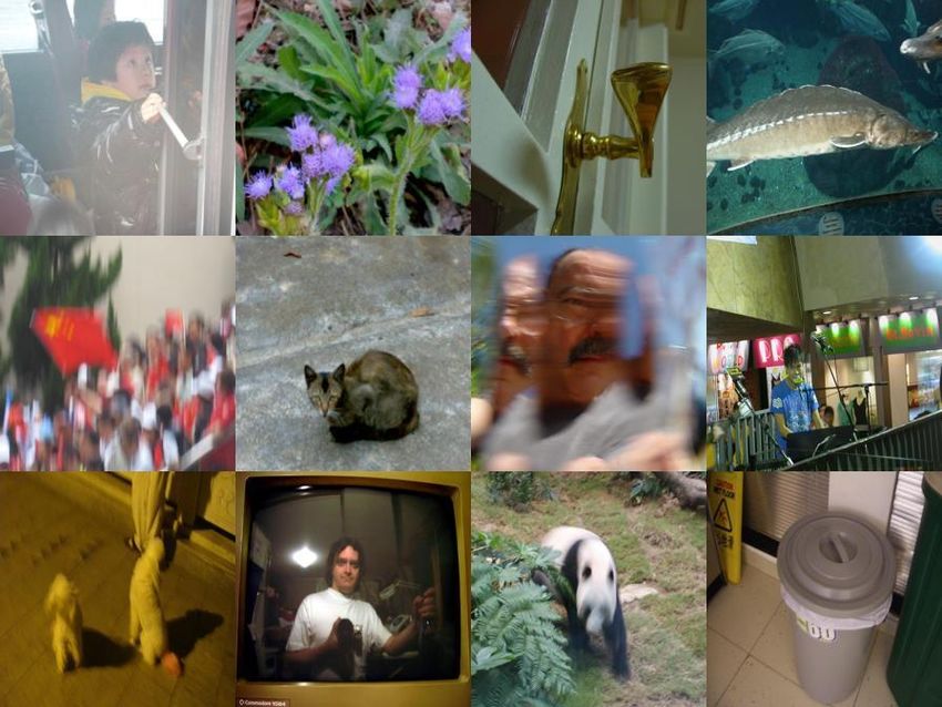

9

subsequently inferred. The BDN model can be considered fully-connected
 convolution Task 1
as an extended version of RAPID that exploits each of
the aesthetic attributes using learned CNN features, hence Task 2
enlarging the parameter space and learning capability of the
overall network.
 Zhang et al. [57] propose a two-column CNN for Fig. 8. A typical multi-task CNN consists of a main task (Task 1) and
learning aesthetic feature representation. The first column multiple auxiliary tasks (only one Task 2 is shown here).
(CN N1 ) takes image patches as input and the second
column (CN N2 ) takes a global image as input. Instead of
randomly sampling image patches given an input image, column CNN combining global composition and salient
a weakly-supervised learning algorithm is used to project a information; the texture CNN takes 16 randomly cropped
set of D textual attributes learned from image tags to highly- patches as input. Category information is predicted using a
responsive image regions. Such image regions in images 3-class SVM classifier before feeding images to a category-
are then fed to the input of CN N1 . This CN N1 contains specific CNN. To alleviate the use of the SVM classifier,
4 convolution layers and one fully-connected layers (f c5 ) an alternative architecture with warped global image as
at the bottom, then a parallel group of D output branches input is trained with a multi-task approach, where the main
(f ci6 , i ∈ {1, 2, ..., D}) modeling each one of the D textual task is aesthetic classification and the auxiliary task is scene
attributes are connected on top. The size of the feature maps category classification.
 Kao et al. [59] propose to learn image aesthetics in a
of each of the f ci6 is of 128-dimensional. A similar CN N2
 multi-task manner. Specifically, AlexNet is used as the base
takes a globally warped image as input, producing one more
 network. Then the 1000-class fc8 layer is replaced by a
128-dim feature vector from f c6 . Hence, the final concate-
 2-class aesthetic prediction layer and a 29-class semantic
nated feature learned in this manner is of 128 × (D + 1)-
 prediction layer. The loss balance between the aesthetic pre-
dimensional. A probabilistic model containing 4 layers is
 diction task and the semantic prediction task is determined
trained for aesthetic quality classification.
 empirically. Moreover, another branch containing two fully-
 Kong et al. [25] propose to learn aesthetic features as-
 connected layers for aesthetic prediction is added to the
sisted by the pair-wise ranking of image pairs as well as
 second convolution layer (conv2 of AlexNet). By linking
the image attribute and content information. Specifically,
 an added gradients flow from the aesthetic task directly to
a Siamese architecture which takes image pairs as input
 convolutional layers, one expects to learn better low-level
is adopted, where the two base networks of the Siamese
 convolutional features. This strategy shares a similar spirit
architecture adopt the AlexNet configurations (the 1000-
 to deeply supervised net [77].
class classification layer fc8 from the AlexNet is removed).
In the first stage, the base network is pre-trained by fine-
tune from aesthetic data using Euclidean Loss regression 7 E VALUATION C RITERIA AND E XISTING R ESULTS
layer instead of softmax classification layer. After that, the Different metrics for performance evaluation of image aes-
Siamese network ranks the loss for every sampled image thetic assessment models are used across the literature:
pairs. Upon convergence, the fine-tuned base-net is used as classification accuracy [20], [21], [23], [24], [25], [40], [43],
a preliminary feature extractor. In the second stage, an at- [47], [49], [50], [52], [53], [54], [55], [56], [57], [58], [59],
tribute prediction branch is added to the base-net to predict [63], [64], [65], [71], [73] reports the proportion of correctly
image attributes information, then the base-net continues classified results; precision-and-recall curve [37], [40], [41],
to be fine-tuned using a multi-task manner by combining [44], [66] considers the degree of relevance of the retrieved
the rating regression Euclidean loss, attribute classification items and the retrieval rate of relevant items, which is
loss and ranking loss. In the third stage, yet another content also widely adopted in image search or retrieval applica-
classification branch is added to the base-net in order to tions; Euclidean distance or residual sum-of-squares error
predict a predefined set of category labels. Upon conver- between the groundtruth score and aesthetic ratings [38],
gence, the softmax output of the content category prediction [70], [71], [74] and correlation ranking [25], [39], [46] are used
is used as a weighting vector for weighting the scores for performance evaluation in score regression frameworks;
produced by each of the feature branch (aesthetic branch, ROC curve [42], [48], [66], [71], [72] and area under the
attribute branch, and content branch). In the final stage, the curve [45], [61], [66] concerns the performance of binary
base-net with all the added output branches is fine-tuned classifier when the discrimination threshold gets varied;
jointly with content classification branch frozen. Effectively, mean average precision [23], [24], [51], [55] is the average
such aesthetic features are learned by considering both the precision across multiple queries, which is usually used
attribute and category content information, and the final to summarize the PR-curve for the given set of samples.
network produces image scores for each given image. These are among the typical metrics for evaluating model
Features learned with Multi-Task CNNs (Fig. 8): Kao et effectiveness on image aesthetic assessment (see Table 1
al. [58] propose three category-specific CNN architectures, for summary). Subjective evaluation by conducting human
one for object, one for scene and one for texture. The surveys is also seen in [62] where human evaluators are
scene CNN takes warped global image as input. It has asked to give subjective aesthetic attribute ratings.
5 convolution layers and three fully-connected layer with We found that it is not feasible to directly compare all
the last fully-connected layer producing a 2-dim softmax methods as different datasets and evaluation criteria are
classification; the object CNN takes both the warped global used across the literature. To this end, we try to summa-
image and the detected salient region as input. It is a 2- rize respectively the released results reported on the two

10

 TABLE 1
 Overview of typical evaluation criteria.
 Method Formula Remarks
 T P +T N Accounting for the proportion of correctly classified samples.
 Overall accuracy P +N T P : true positive, T N : true negative, P : total positive, N : total negative

 1 TP 1 TN Averaging precision and true negative prediction for imbalanced distribution.
 Balanced accuracy +
 2 P 2 N T P : true positive, T N : true negative, P : total positive, N : total negative

 TP TP Measuring the relationship between precision and recall.
 Precision-recall curve p= ,r =
 T P +F P T P +F N T P : true positive, T N : true negative, F P : false positive, F N : false negative

 Measuring the difference between the groundtruth score and aesthetic ratings.
 qP
 Euclidean distance i (Yi − Ybi )2
 Y : ground truth score, Yb : predicted score

 Measuring the statistical dependence between the ranking of aesthetic
 cov(rgX ,rgY )
 Correlation ranking σrgX σrgY prediction and groundtruth.
 rgX , rgY : rank variables, σ : standard deviation, cov : covariance

 Measuring model performance change by tpr (true positive rate) and f pr
 TP FP
 ROC curve tpr = T P +F N
 , f pr = F P +T N
 (false positive rate) when the binary discrimination threshold is varied.
 T P : true positive, T N : true negative, F P : false positive, F N : false negative

 1 Pn The averaged AP values, based on precision and recall.
 Mean average precision i (precision(i) × ∆recall(i))
 n precision(i) is calculated among the first i predictions, ∆recall(i): change in recall

 TABLE 2
 Methods evaluated on the CUHK-PQ dataset.
 Method Dataset Metric Result Training-Testing Remarks
 Su et al. (2011) [72] CUHK-PQ. Overall accuracy 92.06% 1000 training, 3000 testing
 Marchesotti et al. (2011) [47] CUHK-PQ Overall accuracy 89.90% 50-50 split
 Zhang et al. (2014) [67] CUHK-PQ Accuracy 90.31% 50-50 split, 12000 subset
 Dong et al. (2015) [50] CUHK-PQ Overall accuracy 91.93% 50-50 split
 Tian et al. (2015) [54] CUHK-PQ Overall accuracy 91.94% 50-50 split
 Zhang et al. (2016) [57] CUHK-PQ Overall accuracy 88.79% 50-50 split, 12000 subset
 Wang et al. (2016) [53] CUHK-PQ Overall accuracy 92.59% 4:1:1 partition
 Lo et al. (2012) [66] CUHK-PQ Area under ROC curve 0.93 50-50 split
 Tang et al. (2013) [45] CUHK-PQ Area under ROC curve 0.9209 50-50 split
 Lv et al. (2016) [51] CUHK-PQ Mean AP 0.879 50-50 split

standard datasets, namely CUHK-PQ (Table 2) and AVA give a proper number indication of 0.5 × (14k/14k) + 0.5 ×
datasets (Table 3), and present the results on other datasets (0k/6k) = 50% performance on AVA.
in Table 4. To date, the AVA dataset (standard partition) In this regard, in the following sections where we dis-
is considered to be the most challenging dataset by the cuss our findings on a proposed strong baseline, we report
majority of the reviewed work. both overall classification accuracy and balanced accuracy
 The overall accuracy metric appears to be the most in order to get a more reasonable measure of baseline
popular metric. It can be written as performance.
 TP + TN
 Overall accuracy = . (5)
 P +N 8 E XPERIMENTS ON D EEP L EARNING S ETTINGS
This metric alone could be biased and far from ideal as
a Naı̈ve predictor that predicts all examples as positive It is evident from Table 3 that deep learning based ap-
would already reach about (14k + 0)/(14k + 6k) = 70% proaches dominate the performance of image aesthetic as-
classification accuracy. To complement such metric when sessment. The effectiveness of learned deep features in this
evaluating models on imbalanced testing sets, an alternative task has motivated us to take a step back to consider how
balanced accuracy metric [78] can be adopted: in a de facto manner that CNN works in understanding
 the aesthetic quality of an image. It is worth noting that
 1 TP 1 TN training a robust deep aesthetic scoring model is non-trivial,
 Balanced accuracy = ( )+ ( ). (6)
 2 P 2 N and often, we found that ‘the devil is in the details’. To
Balanced accuracy equally considers the classification per- this end, we design a set of systematic experiments based
formance on different classes [78], [79]. While overall ac- on a baseline 1-column CNN and a 2-column CNN, and
curacy in Eq. (5) offers an intuitive sense of correctness evaluate different settings from mini-batch formation to
by reporting the proportion of correctly classified sam- complex multi-column architecture. Results are reported on
ples, balanced accuracy in Eq. (6) combines the prevalence- the widely used AVA dataset.
independent statistics of sensitivity and specificity. A low We observe that by carefully training the CNN archi-
balanced accuracy will be observed if a given classifier tecture, the 2-column CNN baseline reaches comparable or
tends to predict only the dominant class. For the Naı̈ve even better performance with the state-of-the-arts and the
predictor mentioned above, the balanced accuracy would 1-column CNN baseline acquires the strong capability to

11

 TABLE 3
 Methods evaluated on the AVA dataset.
 Method Dataset Metric Result Training-Testing Remarks
 Marchesotti et al. (2013) [48] AVA ROC curve tp-rate: 0.7, fp-rate: 0.4 standard partition
 AVA handcrafted features (2012) [49] AVA Overall accuracy 68.00% standard partition
 SPP (2015) [24] AVA Overall accuracy 72.85% standard partition
 RAPID - full method (2014) [23] AVA Overall accuracy 74.46% standard partition
 Peng et al. (2016) [52] AVA Overall accuracy 74.50% standard partition
 Kao et al. (2016) [58] AVA Overall accuracy 74.51% standard partition
 RAPID - improved version (2015) [55] AVA Overall accuracy 75.42% standard partition
 DMA net (2015) [24] AVA Overall accuracy 75.41% standard partition
 Kao et al. (2016) [59] AVA Overall accuracy 76.15% standard partition
 Wang et al. (2016) [53] AVA Overall accuracy 76.94% standard partition
 Kong et al. (2016) [25] AVA Overall accuracy 77.33% standard partition
 BDN (2016) [56] AVA Overall accuracy 78.08% standard partition
 Zhang et al. (2014) [67] AVA Overall accuracy 83.24% 10%-subset, 12.5k*2
 Dong et al. (2015) [50] AVA Overall accuracy 83.52% 10%-subset, 19k*2
 Tian et al. (2016) [54] AVA Overall accuracy 80.38% 10%-subset, 20k*2
 Wang et al. (2016) [53] AVA Overall accuracy 84.88% 10% subset, 25k*2
 Lv et al. (2016) [51] AVA Mean AP 0.611 10%-subset, 20k*2

 TABLE 4
 Methods evaluated on other datasets.
 Method Dataset Metric Result
 Tong et al. (2004) [20] 29540-image private set Overall accuracy 95.10%
 Datta et al. (2006) [21] 3581-image private set Overall accuracy 75%
 Sun et al. (2009) [38] 600-image private set Euclidean distance 3.5135
 Wong et al. (2009) [63] 3161-image private set Overall accuracy 79%
 Bhattacharya. (2010, 2011) [43], [64] ∼650-image private set Overall accuracy 86%
 Li et al. (2010) [70] 500-image private set Residual sum-of-squares error 2.38
 Wu et al. (2010) [65] 10800-image private set from Flickr Overall accuracy ∼83%
 Dhar et al. (2011) [44] 16000-image private set from DPChallenge PR-curve -
 Nishiyama et al. (2011) [41] 12k-image private set from DPChallenge Overall accuracy 77.60%
 Lo et al. (2012) [42] 4k-image private set ROC curve tp-rate: 0.6, fp-rate: 0.3
 Yeh et al. (2012) [46] 309-image private set Kendalls Tau-b measure 0.2812
 Aydin et al. (2015) [62] 955-image subset from DPChallenge.com Human survey -

 Yin et al. (2012) [73] 13k-image private set from Flickr Overall accuracy 81%
 Lienhard et al. (2015) [71] Human Face Scores 250-image dataset Overall accuracy 86.50%
 Sun et al. (2015) [74] 1000-image Chinese Handwriting Euclidean distance -
 Kong et al. (2016) [25] AADB dataset Spearman ranking 0.6782
 Zhang et al. (2016) [57] PNE Overall accuracy 86.22%

suppress false positive predictions while having competitive backpropagation with stochastic gradient descent, we adopt
classification accuracy. We wish that the experimental re- the cross-entropy classification loss, which is formulated as
sults could facilitate designs of future deep learning models n
for image aesthetic assessment. 1 XX
 L(W) = − {t log p(ybi = t|xi ; W)
 n i=1 t
 (8)
 + (1 − t)log(1 − p(ybi = t|xi ; W)) + φ(W)}
8.1 Formulation and the Base CNN Structure

The supervised learning process of CNNs involves a set exp(wtT xi )
 p(ybi = t|xi ; wt ) = P T
 , (9)
of training data {xi , yi }i∈[1,N ] , from which a nonlinear t0 ∈T exp(wt0 xi )
mapping function f : X → Y is learned through backprop- where t ∈ T = {0, 1} is the ground truth. This formulation is
agation [80]. Here, xi is the input to the CNN and yi ∈ T is in accordance with prior successful model frameworks such
its corresponding ground truth label. For the task of binary as AlexNet [81] and VGG-16 [82], which are also adopted as
classification, yi ∈ {0, 1} is the aesthetic label corresponding the base network in some of our reviewed approaches.
to image xi . The convolutional operations in such a CNN
 The original last fully-connected layer of these two net-
can be expressed as
 works are for the 1000-class ImageNet object recognition
 challenge. For aesthetic quality classification, a 2-class aes-
 Fk (X) = max(wk ∗ Fk−1 (X) + bk , 0), k ∈ {1, 2, ..., D} (7) thetic classification layer to produce a soft-max predictor is
 needed (see Fig. 9a). Following typical CNN approaches,
where F0 (X) = X is the network input and D is the the input size is fixed to 224 × 224 × 3, which are cropped
depth of the convolutional layers. The operator ’∗’ denotes from a globally warped 256 × 256 × 3 images. Standard data
the convolution operation. The operations in the D0 fully- augmentation such as mirroring is performed. All baselines
connected layers can be formulated in a similar manner. To are implemented based on the Caffe package [83]. For clarity
learn the (D + D0 ) network weights W using the standard of presentation in the following sections, we name the all