Design and Implementation of a Recommender System for News in - Accso
←
→
Page content transcription
If your browser does not render page correctly, please read the page content below

Design and Implementation of a
Recommender System for News in
ZDFMEDIATHEK based on Deep
Reinforcement Learning
Konzeption und Implementierung eines Empfehlungsverfahrens für Nachrichten in der
ZDFMEDIATHEK auf Basis des tiefen verstärkenden Lernens
Master-Thesis von Valentin Kuhn aus Franfurt am Main
18. November 2019

                                                                  Fachbereich Informatik
                                                                  Knowledge Engineering Group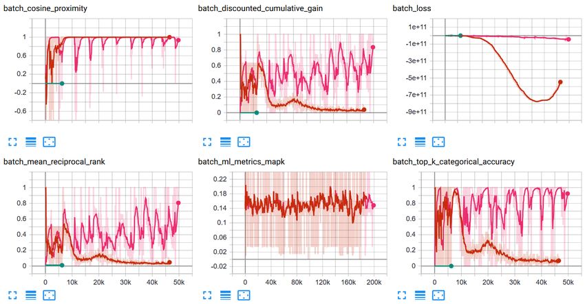
Design and Implementation of a Recommender System for News in ZDFMEDIATHEK based on Deep
Reinforcement Learning
Konzeption und Implementierung eines Empfehlungsverfahrens für Nachrichten in der
ZDFMEDIATHEK auf Basis des tiefen verstärkenden Lernens

Vorgelegte Master-Thesis von Valentin Kuhn aus Franfurt am Main

1. Gutachten: Prof. Dr. Johannes Fürnkranz
2. Gutachten: Tobias Joppen

Tag der Einreichung: 18. November 2019
Erklärung zur Abschlussarbeit gemäß § 23 Abs. 7 APB der TU Darmstadt

Hiermit versichere ich, Valentin Kuhn, die vorliegende Master-Thesis ohne Hilfe Dritter und nur
mit den angegebenen Quellen und Hilfsmitteln angefertigt zu haben. Alle Stellen, die Quellen
entnommen wurden, sind als solche kenntlich gemacht worden. Diese Arbeit hat in gleicher oder
ähnlicher Form noch keiner Prüfungsbehörde vorgelegen.

Mir ist bekannt, dass im Fall eines Plagiats (§ 38 Abs. 2 APB) ein Täuschungsversuch vorliegt,
der dazu führt, dass die Arbeit mit 5,0 bewertet und damit ein Prüfungsversuch verbraucht wird.
Abschlussarbeiten dürfen nur einmal wiederholt werden.

Bei der abgegebenen Thesis stimmen die schriftliche und die zur Archivierung eingereichte
elektronische Fassung überein.

Bei einer Thesis des Fachbereichs Architektur entspricht die eingereichte elektronische Fassung
dem vorgestellten Modell und den vorgelegten Plänen.

 Datum / Date:                         Unterschrift / Signature:

                                       (Valentin Kuhn)
Abstract Tremendous supply of online content puts a strain on users by overburdening their capabilities to filter interesting content. Therefore, over-the-top providers recognized a growing need for per- sonalized recommendations. Especially in fast-paced domains, such as news, up-to-date filtering is crucial for user satisfaction. The domain of news recommendation features two characteristics setting it apart from many other recommendation applications: a dynamically changing corpus of items and user preference, and, rewards not necessarily coupled to immediate click-through rates. Thus, we describe a novel approach recently introduced by Zheng et al. [60] that explicitly considers these two limitations of prior recommendation engines in a deep Q-learning approach with Dueling Bandit Gradient Descent for exploration. Furthermore, we adapt the application of the presented deep Q-network to ZDFMEDIATHEK.
Contents

1 Introduction                                                                                                                                                                                1

2 Background                                                                                                                                                                                  5
  2.1 Prior Work . . . . . . . . . . . . . . . . . . .                                   .   .   .   .   .   .   .   .   .   .   .   .   .   .   .   .   .   .   .   .   .   .   .   .   .    5
  2.2 Preliminaries . . . . . . . . . . . . . . . . . .                                  .   .   .   .   .   .   .   .   .   .   .   .   .   .   .   .   .   .   .   .   .   .   .   .   .    7
      2.2.1 Reinforcement Learning . . . . . .                                           .   .   .   .   .   .   .   .   .   .   .   .   .   .   .   .   .   .   .   .   .   .   .   .   .    7
      2.2.2 Neural Networks & Deep Learning                                              .   .   .   .   .   .   .   .   .   .   .   .   .   .   .   .   .   .   .   .   .   .   .   .   .    9
      2.2.3 Deep Reinforcement Learning . . .                                            .   .   .   .   .   .   .   .   .   .   .   .   .   .   .   .   .   .   .   .   .   .   .   .   .   11

3 Technique: DDQN                                                                                                                                                                            13
  3.1 Recommendation Pipeline . . . . . . . . .                                      .   .   .   .   .   .   .   .   .   .   .   .   .   .   .   .   .   .   .   .   .   .   .   .   .   .   14
  3.2 Model Architecture . . . . . . . . . . . . .                                   .   .   .   .   .   .   .   .   .   .   .   .   .   .   .   .   .   .   .   .   .   .   .   .   .   .   14
  3.3 Input Features . . . . . . . . . . . . . . . .                                 .   .   .   .   .   .   .   .   .   .   .   .   .   .   .   .   .   .   .   .   .   .   .   .   .   .   16
  3.4 Network Layers . . . . . . . . . . . . . . .                                   .   .   .   .   .   .   .   .   .   .   .   .   .   .   .   .   .   .   .   .   .   .   .   .   .   .   19
  3.5 Loss Function . . . . . . . . . . . . . . . .                                  .   .   .   .   .   .   .   .   .   .   .   .   .   .   .   .   .   .   .   .   .   .   .   .   .   .   21
      3.5.1 Categorical Cross-entropy Loss .                                         .   .   .   .   .   .   .   .   .   .   .   .   .   .   .   .   .   .   .   .   .   .   .   .   .   .   21
      3.5.2 Binary Cross-Entropy Loss . . . .                                        .   .   .   .   .   .   .   .   .   .   .   .   .   .   .   .   .   .   .   .   .   .   .   .   .   .   22
  3.6 Reward . . . . . . . . . . . . . . . . . . . .                                 .   .   .   .   .   .   .   .   .   .   .   .   .   .   .   .   .   .   .   .   .   .   .   .   .   .   22
      3.6.1 Offline Reward . . . . . . . . . . .                                     .   .   .   .   .   .   .   .   .   .   .   .   .   .   .   .   .   .   .   .   .   .   .   .   .   .   22
      3.6.2 Online Reward . . . . . . . . . . .                                      .   .   .   .   .   .   .   .   .   .   .   .   .   .   .   .   .   .   .   .   .   .   .   .   .   .   23
  3.7 Exploration . . . . . . . . . . . . . . . . . .                                .   .   .   .   .   .   .   .   .   .   .   .   .   .   .   .   .   .   .   .   .   .   .   .   .   .   25
      3.7.1 Epsilon-Greedy . . . . . . . . . . .                                     .   .   .   .   .   .   .   .   .   .   .   .   .   .   .   .   .   .   .   .   .   .   .   .   .   .   25
      3.7.2 Dueling Bandit Gradient Descent                                          .   .   .   .   .   .   .   .   .   .   .   .   .   .   .   .   .   .   .   .   .   .   .   .   .   .   25

4 Implementation                                                                                          29
  4.1 Frameworks . . . . . . . . . . . . . . . . . . . . . . . . . . . . . . . . . . . . . . . . . . . 30
  4.2 Environment . . . . . . . . . . . . . . . . . . . . . . . . . . . . . . . . . . . . . . . . . . . 32
  4.3 Agent . . . . . . . . . . . . . . . . . . . . . . . . . . . . . . . . . . . . . . . . . . . . . . . 33

5 Evaluation                                                                                                                                                                                 35
  5.1 Experiment Setup .         .   .   .   .   .   .   .   .   .   .   .   .   .   .   .   .   .   .   .   .   .   .   .   .   .   .   .   .   .   .   .   .   .   .   .   .   .   .   .   36
  5.2 Hyperparameters .          .   .   .   .   .   .   .   .   .   .   .   .   .   .   .   .   .   .   .   .   .   .   .   .   .   .   .   .   .   .   .   .   .   .   .   .   .   .   .   36
  5.3 Data . . . . . . . . .     .   .   .   .   .   .   .   .   .   .   .   .   .   .   .   .   .   .   .   .   .   .   .   .   .   .   .   .   .   .   .   .   .   .   .   .   .   .   .   37
  5.4 Experiment Results         .   .   .   .   .   .   .   .   .   .   .   .   .   .   .   .   .   .   .   .   .   .   .   .   .   .   .   .   .   .   .   .   .   .   .   .   .   .   .   37

6 Related Work                                                                                                                                                                               41

7 Conclusion                                                                                                                                                                                 45

Acronyms                                                                                                                                                                                      V

References                                                                                                                                                                                   VII

                                                                                                                                                                                               I
List of Figures
1 Recommendations in ZDFmediathek . . . . . . . . . . . . . . . . . . . . . . . . . . . . 1
2 Reinforcement Learning in Recommender Systems . . . . . . . . . . . . . . . . . . . . 2
3 Candidate Generation in Recommender Systems . . . . . . . . . . . . . . . . . . . . . 3
4 Comparison of Contextual Multi-Armed Bandit and Markov Decision Process . . . 6
5 Agent and Environment in the Markov Decision Process . . . . . . . . . . . . . . . . 7
6 Artificial Neuron in a Multilayer Perceptron . . . . . . . . . . . . . . . . . . . . . . . . 10
7 Recommender-User Interactions in the Markov Decision Process . . . . . . . . . . . 11
8 Conceptual View on the Technique in MDP . . . . . . . . . . . . . . . . . . . . . . . . 13
9 Candidate Generation in ZDFmediathek . . . . . . . . . . . . . . . . . . . . . . . . . . 14
10 Comparison of Network Architectures . . . . . . . . . . . . . . . . . . . . . . . . . . . 15
11 Dueling Deep Q-Network Architecture in ZDFmediathek . . . . . . . . . . . . . . . . 16
12 Model Architecture of the Double Dueling Deep Q-Network . . . . . . . . . . . . . . 18
13 Comparison of ReLU Activations . . . . . . . . . . . . . . . . . . . . . . . . . . . . . . . 20
14 User Activeness Estimation for a User . . . . . . . . . . . . . . . . . . . . . . . . . . . . 24
15 Conceptual View on the Technique in MDP . . . . . . . . . . . . . . . . . . . . . . . . 29
16 Dockerfile preparing our Tensorflow docker image . . . . . . . . . . . . . . . . . . . . 30
17 Keras Summary of the Q-network . . . . . . . . . . . . . . . . . . . . . . . . . . . . . . 31
18 Building simulator memory . . . . . . . . . . . . . . . . . . . . . . . . . . . . . . . . . . 32
19 Conceptual View on the Simulator Environment . . . . . . . . . . . . . . . . . . . . . 35
20 Training Metrics . . . . . . . . . . . . . . . . . . . . . . . . . . . . . . . . . . . . . . . . . 38
21 Comparison of Deep Q-Network Architectures . . . . . . . . . . . . . . . . . . . . . . 41
IIIFigure 1: Recommendations in ZDFMEDIATHEK
1 Introduction
Recent improvements in communication technology and increasing user interests in non-linear
streaming services have led to an enormous growth in online content, especially in Over-The-
Top (OTT) media services. OTT services directly distribute content to users without intermediary
distributors or platforms. For instance, Covington et al. [9] describe video recommendations out
of a huge corpus for over a billion users of YouTube and Zheng et al. [60] points to a similarly
scaled volume of items in Google News. This tremendous amount of online content can be
overwhelming for users, providing too many choices for a user to grasp an overview of all the
content provided. Thus, personalized content recommendation improves user experience by
narrowing the corpus of content for the user to efficiently decide on which content to consume
next. Specifically, OTT television services such as ZDFMEDIATHEK1 put much manual labor into
curation of the contents in their media platform. Automation of this time-consuming task could
free resources for more content production or improved quality assurance.
Contrary to many recommendation scenarios in other domains including online shopping and
movie databases, news recommendation needs to rapidly adapt to a changing corpus of news
to recommend, since news are outdated quickly. According to Zheng et al. [60], news are only
of interest during the first 4.1 hours after publication. Furthermore, user preference in certain
topics of news often changes over time [60]. For instance, a user may be interested in weather
updates in the morning and a daily recap in the evening. Furthermore, preferences may change
over larger periods of time, e.g., during different seasons or events such as soccer tournaments.
These dynamics are impossible to handle manually and further prove the necessity of automation
in news recommendation at ZDFMEDIATHEK.
Besides, personalized recommendations directly impacts economical development of a plat-
form: Lamere and Green [25] reported that 35% of all sales on Amazon originated from recom-
mended products and Das et al. [10] increased traffic on Google News by 38% by introducing a
personalized recommender system. Similarly, ZDF as a publicly held company aims to increase
usage of ZDFMEDIATHEK in order to defend public funding into its services and, possibly, advo-
cate increased public funding in the future. Therefore, ZDFMEDIATHEK already shows a row of
recommendations on its home page, as shown in Figure 1. Typically, these recommendations
are ranked individually for each user.
Recommender systems take into account the content already consumed by a certain user in
order to recommend them new items from a corpus of consumable items. Such systems solely
relying on content, i.e., Content-Based (CB) approaches, often exhibit inferior performance com-
pared to techniques utilizing both content similarities and user similarities, i.e., Collaborative
1
ZDFmediathek: https://zdf.de
1Recommender
recommendation
state s t reward r t
(action) a t
r t+1
Users
s t+1
Figure 2: Reinforcement Learning in Recommender Systems
Filtering (CF) approaches. While improving on CB systems, CF approaches consider user prefer-
ences as static and, thus, are limited in their effectiveness in the dynamic nature of news recom-
mendations. For instance, a user may be very interested in news about a particular thunderstorm
approaching his location, which does not necessarily indicate a long-lasting user preference in
thunderstorms. Besides, CB approaches require a dense item-to-item similarity matrix and CF
techniques are based on user-item matrices. Data for these matrices is often sparse and, thus,
most prior work does not handle the fast pace of news items appearing and becoming irrelevant.
Furthermore, both CB and CF maximize immediate rewards such as click-through rates instead
of taking into account long-term benefits such as user activeness on the platform or user return
patterns. To counter these limitations, recent approaches in news recommendation utilize Deep
Learning (DL) to learn more complex user-item interactions and apply Reinforcement Learning
(RL) for considering expectations of future rewards in addition to immediate rewards [31; 60].
The aforementioned combination of improvements in user experience, increase in productivity
and economic growth through recommendations and limitations of state-of-the-art approaches
convinced ZDFMEDIATHEK to implement a DL based approach specifically for news recommenda-
tions. Zheng et al. [60] propose a novel approach using Deep Q-Learning to solve the online
personalized news recommendation problem. News recommendation requires a system to han-
dle dynamic changes instead of a static corpus of content, user activity instead of click labels and
diversification instead of recommending similar items. Therefore, Zheng et al. [60] propose a
Double Dueling Deep Q-Network (DDQN) framework to solve these challenges by continuously
retraining through RL, explicitly considering future reward, maintaining a user activeness score
and pursuing more exploration using a Dueling Bandit Gradient Descent (DBGD) method.
RL adequately handles a dynamically changing corpus of news and user preferences by con-
tinuously retraining the learning model. Figure 2 depicts the interaction of the recommender
system with the users in a RL context. The recommender system provides recommendations to
the users. Afterwards, the users provide feedback on the recommendations by either explicitly
rating or implicitly clicking and consuming the recommended items. The recommender system
receives this feedback as reward for the provided recommendations and, furthermore, receives
an updated state with current user preferences and an extended corpus of news to recommend.
Obviously, this system has a drawback: in the beginning, the recommender system needs to
provide recommendations without “knowing” the state and reward. We handle this cold-start
problem by pre-training the DDQN in an offline simulator based on recorded user interactions in
ZDFMEDIATHEK.
2User &
Context
Corpus Candidate
Ranking Item List
of News Generation
Figure 3: Candidate Generation in Recommender Systems [c.f., 9, p. 2]
The underlying Deep Q-Network (DQN) of Zheng et al. [60] utilizes Q-learning to decide on a
ranking for recommended items. The DQN assigns a Q-value to each item in the corpus denoting
the item’s probability of bearing a high reward, i.e., being clicked or increasing user activeness
on the platform. Unfortunately, this requires each item in the corpus to be put into the DQN to
predict a Q-value. Since this does not scale well for large corpora, we only calculate Q-values
for a pre-determined set of candidates. Figure 3 shows the pipeline starting with the corpus of
news. Next, the pipeline passes the candidate generation that reduces the amount of items to be
considered in the ranking step. This ranking step produces a ranked list of recommended items
considering the context and the requesting user’s preferences and history. In other domains apart
from news recommendation, complex candidate generation methods may be necessary. But due
to the very dynamic nature of news, which are outdated after only 4.1 hours, naïvely selecting
the freshest news as candidates is adequate [60]. Furthermore, we represent states and actions
in continuous spaces, allowing for consideration of previously unknown state and action features
in the recommendation procedure. Thus, the DQN appropriately handles arbitrary candidates.
To sum up, we aim to recreate the DDQN approach by Zheng et al. [60] featuring two du-
eling Deep Q-Networks in a double Deep Q-Network architecture and an exploration DQN in
Dueling Bandit Gradient Descent. Unfortunately, recreation of published papers’ results is often
complex and challenging, although it assures scientific confirmability and interpretability [3].
Furthermore, we aim to adapt this approach to a similar domain, ZDFMEDIATHEK, which provides
sufficient data and allows to test transferability of the DDQN agent to similar domains.
The following thesis is structured as follows: first, section 2 examines existing approaches
and provides preliminaries for Reinforcement Learning, Deep Learning and the combination of
both in Deep Q-Networks. Second, we present our model architecture of the DDQN adapted for
ZDFMEDIATHEK in section 3. Next, we discuss implementation details and evaluation details in
section 4 and section 5 respectively. Finally, we present closely related work in section 6 and
come to a conclusion in section 7.
34
2 Background
Since news recommendations are a very narrow field of studies, we reference prior work on
generating recommendations in general, narrowing down to Reinforcement Learning based ap-
proaches and, finally, name a few news recommendation techniques. Furthermore, we provide
the theoretical fundamentals required for the Double Dueling Deep Q-Network utilized in our
technique.

2.1 Prior Work
Recommender systems have been studied extensively, providing numerous existing approaches.
These approaches include content-based filtering [39], matrix-factorization-based methods [11;
24; 30; 53], logistic regression [36], factorization machines [19; 40] and, recently, deep learning
models [9; 31; 54; 60].
   Content-based filtering recommends items by considering content similarity between items
[39]. In contrast, Collaborative Filtering (CF) recommends items preferred by users with simi-
lar behaviour and assumes that similar users tend to provide the same ratings for items. Thus,
conventional CF-based methods rely heavily on existing ratings to calculate similarities in order
to provide reliable recommendations and, therefore, are prone to errors through scarce data.
Recommender systems often make use of advanced CF-based methods such as Matrix Factor-
ization (MF). MF represents both items and users as vectors in the same space [11; 24; 30;
53]. Besides, recommendation may be presented as binary classification problem, i.e., whether
to recommend an item or not. Logistic Regression (LR) solves such binary decision problems.
However, LR-based approaches are „hard to generalize to the feature interactions that never
or rarely appear in the training data“ [c.f. 31, p. 3]. Conversely, Factorization Machines (FM)
show promising results even on scarce data by modeling pairwise feature interactions as inner
product of latent vectors corresponding to features. Recently, the complex feature interactions
for recommendation procedures were learned by deep learning models [9; 31; 54; 60].

Contextual Multi-Armed Bandits for Recommendations
   Additionally to previously mentioned approaches, Contextual Multi-Armed Bandit (MAB) mod-
els were utilized to generate recommendations [7; 27; 52; 57; 59]. MABs are a group of recom-
mender systems, that select a different arm, i.e., recommendation technique, for each request
based on the probability of this arm’s recommendations yielding a high reward. In Contextual
MABs depicted in Figure 4a, the bandit considers the context, i.e., certain features concerning the
bandit’s task, when selecting one of its arms. For news recommendations, this context contains
both user and item features. Zeng et al. [57] already considers dynamic user preferences varying
over time.
   However, all previously named approaches, including CF, MF, LR, FM, and, Contextual MABs,
face two limitations regarding news recommendations.
  1. These approaches consider the user’s preference as static and aim to learn this preference
     as precise as possible.
In news recommendation, user interest is especially volatile and even changes in the course of a
single day [60]. Thus, the recommendation procedure cannot be modeled as static process.
  2. Furthermore, all aforementioned techniques aim to maximize immediate rewards, e.g., user
     clicks.

                                                                                                 5
context c t Recommender
Recommender
(Bandit)
(Agent)
recommendation recommendation
reward r t state s t reward r t
(action) a t (action) a t
r t+1 r t+1
Users Users
(Environment) (Environment)
s t+1
(a) Recommender-User interactions of a (b) Recommender-User interactions in the
Contextual Multi-Armed Bandit Markov Decision Process
Figure 4: Comparison of Contextual Multi-Armed Bandit and Markov Decision Process
Only considering immediate rewards could harm recommendation performance in the long term.
In addition to immediate rewards, we aim to account for long-term benefits of recommendations
such as increasing user activeness on the platform under consideration.
Reinforcement Learning for Recommendations
Furthermore, Reinforcement Learning (RL) was applied to recommendation scenarios as
Markov Decision Process (MDP) models. In the MDP, an agent selects actions based on his percep-
tion of the environment to improve the agent’s position in the environment. The agent’s position
is calculated based on reward received from the environment after presenting the selected ac-
tions. As shown in Figure 4b, a recommender system acts as the agent in RL recommendations.
The agent’s action space is represented by the item space from which the recommender system
selects the best items to present to the users, who act as an MDP environment. Based on the
recommended items, users generate rewards for the recommender system, e.g., by clicking rec-
ommended items. Next, the recommender system receives this reward and, in contrast to the
previously described Contextual MAB, also perceives the new state created through the recom-
mender’s user interaction. The recommender system continuously adapts its recommendation
policy to generate recommendations yielding a higher reward.
Contrary to Contextual MABs, agents in an MDP are capable of considering potential future
rewards [60]. Many previous approaches try to model the items as state and the transition
between items as action, leading to an exploding state space for larger corpora of items [32; 34;
41; 45; 49]. Furthermore, training these models is limited by sparse transitions data [31; 60].
In contrast to prior work, we design continuous state and action spaces, which allows for scaling
of the corpus of news and is robust to sparse interaction data.
6Agent
state s t reward r t action a t = πθ (s t )
r t+1
Environment
s t+1
Figure 5: Agent and Environment in the Markov Decision Process [31]
2.2 Preliminaries
Since our technique combines multiple machine learning paradigms, such as a Q-learning ap-
proach to Reinforcement Learning and Artificial Neural Networks in a Deep Learning manner,
we first introduce the theoretical fundamentals of these paradigms. Next, we describe how these
paradigms are combined in a Deep Q-Network for Deep Reinforcement Learning.
2.2.1 Reinforcement Learning
An agent in a Reinforcement Learning (RL) scenario interacts with its environment over time,
thus, the agent reinforces its behaviour by continuously learning new information based on its
(inter-)actions and the environment’s reaction. A Reinforcement Learning agent is formalized
in the Markov Decision Process (MDP). We define an MDP as (S, A, P, R, γ) with
• S denoting the state space,
• A denoting the action space,
• P : S × A × S 7→ [0, 1] denoting the state transition function,
• R : S × A × S 7→ R denoting the reward function, and,
• γ denoting the discount rate
of the agent [1; 28; 29; 31; 48]. Figure 5 visualizes an agent in an MDP: At each time
step t, the agent receives a state s t ∈ S and selects an action a t ∈ A following a policy
πθ (a t |s t ) : S × A 7→ [0, 1] describing the agent’s behavior. In the next time step, the agent
receives state s t+1 ∈ S, following the agents behavior (selection of a) and environmental dynam-
ics modeled in P (s t , a t , s t+1 ). Finally, the agent receives a reward r t according to the reward
function R (s t , a t , s t+1 ).
Temporal Difference Learning
Generally, an agent in an MDP aims to find an optimal policy (π∗ : S × A 7→ [0, 1]) which
maximizes the expected cumulative rewards from any state s ∈ S, i.e.,
¨∞ «
∑
V ∗ (s) = max Eπθ γt rt . (1)
πθ
t=0
7Here, V ∗ (s) is the value of state s under the optimal policy, Eπθ is the expectation under policy
πθ , t is the current time step and r t is the reward at time step t discounted by the discount rate
γ. Discounting by γ t values immediate rewards higher than expected future rewards to account
for uncertainty of the future.
A central aspect of RL is temporal difference learning, which allows to learn the value function
V (s) directly from the temporal difference error V (s t+1 ) − V (s t ) through value iteration of the
Bellman approximation
Vs ← r + γ max Vs′ (2)
a′ ∈A
for each tuple of state s, action a, reward r for the action and next state s′ [47]. The Bell-
man approximation in Equation 2 approximates the Bellman equation of optimality V0 ←
maxa∈1...N (ra + γVa ) which Richard Bellman proved to always find the optimal policy [2]. For
smoother convergence of Vs , we blend old and new values
Vs ← (1 − α)Vs + α(r + γ max Vs′ ) (3)
a′ ∈A
given a constant step-size parameter α ∈ (0, 1], also known as learning rate in the machine
learning context [26; 28; 29; 48, pp. 25, 97].
Q-Learning
Equivalently to maximizing V (s) in temporal difference learning, an agent in an MDP may
maximize the expected cumulative rewards from any state-action pair {(s, a) | s ∈ S, a ∈ A}, i.e.,
¨∞ «
∑
Q∗ (s, a) = max Eπθ γt rt . (4)
πθ
t=0
Here, Q∗ (s, a) is the value of taking action a in state s under the optimal policy, Eπθ is the
expectation under policy πθ , t is the current time step and r t is the immediate reward at time
step t discounted by the discount rate γ. Again, discounting is applied to account for uncertainty
of the future.
Similarly to value iteration, we can directly learn Q(s, a) from the temporal difference error in
a process named Q-Learning through the Bellman approximation
Q s,a ← r + γ max Q s′ ,a′ (5)
a′ ∈A
since V ∗ (s) = maxa Q∗ (s, a) holds [48, pp. 51, 107; 56]. Analogous to value iteration, we blend
old and new values of Q s,a for smoother convergence
Q s,a ← (1 − α)Q s,a + α(r + γ max Q s′ ,a′ ). (6)
a′ ∈A
The basic form of Q-learning is tabular Q-learning, which describes learning a state-action
table of Q-values, where each cell contains the Q-value for the respective action in the corre-
sponding state. Thus, the table includes return values of Q(s, a) for all combinations of s and
a. For instance, in a game of Tic-Tac-Toe each row of the table corresponds to one state of the
board and each column of the table represents putting a marker on one of the fields. Tabular
Q-learning starts with an empty table in state s0 and repeatedly performs the Bellman update as
described in Equation 6 to fill the cells [26, p. 121]. After multiple iterations of Q-learning, the
agent’s Q-table may contain similar Q-values to the following table:
8Q-Table of Tic-Tac-Toe
Top Top Center Bottom
State ... ...
Left Center Center Right
s0 = 0.8 0.4 ... 0.1 ... 0.7
×
s1 = 0.0 0.1 ... 0.9 ... 0.2
... ... ... ... ... ... ... ...
Here, bold Q-values represent the best action in each state, i.e. maxa Q(s t , a). Thus, as shown
in the first row, the agent would start the game by putting its marker in the top left cell of the
board, i.e., argmaxa Q(s0 , a). If the agent needed to react to the out-coming state s1 as shown
in the second row, the agent would put its marker into the center of the board. We omitted all
further states and actions for comprehensibility.
Naturally, learning a Q-table works well for relatively small and static state and action spaces
such as Tic-Tac-Toe. For large state and action spaces as in recommender systems, the Q-table
approach is by far too memory-intensive. Furthermore, Q-tables cannot handle dynamic state
and action spaces and struggle with sparse information. Thus, recommendations are only pos-
sible with a more efficient and robust approach, e.g., by approximating the Q-function with an
Artificial Neural Network.
Sutton and Barto [48] provide proves and an in-depth explanation on Reinforcement Learning
beyond the scope of this thesis. Additionally, Géron [12] and Lapan [26] provide insight about
practical implications of RL, temporal difference learning and Q-learning.
2.2.2 Neural Networks & Deep Learning
As Deep Learning (DL) is a specialized technique utilizing Artificial Neural Networks (ANNs),
we first describe the foundations of neural networks. An ANN consists of a multitude of artificial
neurons which are connected through synapses as shown in Figure 6, following the nomenclature
of a human brain [21]. Each neuron has one or more inputs, an activation threshold and at least
one output that sends a signal via a synapse to another neuron upon activation. The connection
of multiple neurons and synapses is called perceptron. Usually, perceptrons are organized into
multiple interconnected layers in a Multilayer Perceptron (MLP), the base architecture of a trivial
ANN.
Formally, a neuron has multiple inputs x 1 , x 2 , ..., x n weighted with corresponding weights
w1 , w2 , ..., w n , as depicted on the left side of Figure 6. Additionally, each neuron has a bias,
represented ∑nby (+1) × w0 . The neuron calculates the sum of the bias and all weighted inputs,
i.e., w0 + i=1 w i x i . This sum is used as input of the neuron’s activation function σ. Here, σ
acts as an activation threshold that controls whether the neuron is activated and “fires” a signal
to all dependent neurons.
The right side of Figure 6 shows the interdependence of neurons. The neurons are organized
into layers. Here, the inputs I1 , I2 , I3 each reach one neuron in the input layer. Each neuron in
9Input Hidden Output
layer layer layer
+1 w
0
w ∑
n I1 O1
x1 1 σ w0 + wi x i
w2 i=1 I2
x2 Σσ
w3 I3 O2
x3
..
n
.
w
xn
Figure 6: Artificial Neuron in a Multilayer Perceptron [51]
the input layer then applies its activation function and feeds the output to all neurons in the
so-called hidden layer, which is not “visible” from the outside because no inputs or outputs are
connected to its neurons. Each neuron in the hidden layer applies its activation function to its
inputs and feeds the result to both neurons in the output layer. Finally, the neurons in the output
layer produce the outputs O1 , O2 by applying their activation functions. Naturally, this model is
called Multilayer Perceptron since it is a perceptron consisting of multiple layers of neurons, or
Feed-Forward Neural Network, since all synapses feed-forward to the following layer instead of
allowing recurrent connections.
The number of neurons per layer determines the width of this layer, while the number of layers
determines the depth of the neural network. Deep Learning utilizes “deep” neural networks, thus,
ANNs with multiple hidden layers [14].
Such ANN is usually trained through a process called backpropagation [44, p. 1]. Basically,
backpropagation trains an ANN by adjusting the weights of the synapses between neurons „in
proportion to the product of their simultaneous activation“ [c.f. 35, p. 1], thus, „propagating
corrections back towards the sensory end [i.e., input layer] of the network if it fails to make
a satisfactory correction quickly at the response end [i.e., output layer]“ [43, p. 292]. Since
backpropagation adjusts the weights through gradient descent on the ”propagated corrections“,
all activation functions in the ANN need to be differentiable.
First, the network is fed-forward from the input layer to the output layer with a training ex-
ample to infer a prediction. During the feed-forward step, each neuron stores its output and
partial derivatives of its activation function for each input. At the output layer, a loss function
E is applied to the predicted output and the expected output, calculating the error. Afterwards,
this error is backpropagated iteratively through the network: for each weight w i j at the synapse
from neuron i with output oi to neuron j the gradient of the loss function is calculated as
∂E ∂E
= oi = oi δ j (7)
∂ wi j ∂ oi w i j
where δ j denotes the backpropagated error up to neuron j. Once all partial derivatives of E have
been computed, the weights w i j are updated via gradient descent:
w∗i j = w i j − γoi δ j (8)
with learning rate γ to only train the network towards the current training example but keep
experience from previous examples.
10Recommender
(Agent)
recommendation
state s t reward r t
(action) a t = πθ (s t )
r t+1
Users
(Environment)
s t+1
Figure 7: Recommender-User Interactions in the Markov Decision Process [31]
Rojas [42] more thoroughly describes and proves the backpropagation algorithm in more com-
plex network architectures and various forms of model formalization, i.e., in matrix form.
2.2.3 Deep Reinforcement Learning
Deep Reinforcement Learning describes approaches utilizing Deep Learning to train an agent in
a Reinforcement Learning context, which has already proven to be beneficial in music recom-
mendation [54] and YouTube video recommendation [9].
Often, Deep Learning techniques are utilized to approximate the Q-value described in sub-
subsection 2.2.1 in an approach named Deep Q-Network (DQN) [38]. To achieve this, an ANN
is used for the agent’s implementation. Since ANNs require vast amounts of training data, the
agent may be pre-trained on historical data of interactions from a similar agent with the envi-
ronment before starting the actual RL process to refine the agent over time. Afterwards, this
ANN is an approximator for the Q-function under the optimal policy Q∗ (s, a) (c.f., Equation 4).
In a recommendation scenario, the RL terminology may be replaced by the corresponding
terms from recommender engines. As shown in Figure 7, we map the recommendation procedure
onto a sequential decision making problem where the recommender acts as an agent, providing
recommendations instead of actions to users, who act as an Environment by providing feedback
on the recommendations via clicks, ratings or consumption times. The recommender uses the
quantified user feedback as reward for past recommendations to improve in the future.
11Corpus Deep
of News Q-Network
L
Target
Network
Probabilistic
Deep Interleave
DDQN
Q-Network
Explore
Network eL
example
Agent
Recorded
Click Log state
action
reward
offline Users
Environment
online
Figure 8: Conceptual View on the Technique in MDP
3 Technique: DDQN
Previous methods lack key features for news recommendation, especially regarding adaptability
to a dynamically changing corpus of content, consideration of user activity and activeness in-
stead of click labels or ratings and diversification to also present different, up-to-date news and
prevent formation of a filter bubble [60]. Therefore, we examine a novel approach by Zheng
et al. [60] specifically designed for news recommendation and adapt the approach to data and
requirements found in a commercial real-world scenario: ZDFMEDIATHEK2 . The news domain of-
fers a specifically large corpus of items for recommendation. Furthermore, this corpus of news
items is very dynamic, requiring continuous updates of the recommendation engine. Besides,
user preferences change quickly based on context, i.e., time of day, day of week or season. For
instance, a user may only be interested in soccer during international tournaments, requiring the
recommender engine to explicitly consider user preference in the recommendation procedure.
Figure 8 presents a conceptual view on our technique. Naturally, we depend on the corpus of
news shown in the top left. Besides, we clearly differentiate between an offline part on the left
and an online part on the right. Here, we apply machine learning terminology, where “offline”
learning has access to all data from the beginning in contrast to “online” learning, where data
becomes available sequentially during the training process.
2
ZDFmediathek: https://zdf.de
13User &
Context
1 & 200
Corpus * Candidate 200 10
Ranking Item List
of News Generation
Figure 9: Candidate Generation in ZDFMEDIATHEK [c.f., 9, p. 2]
In offline training, we train the Deep Q-Network (DQN) on examples extracted from a click log
of previously recorded user interactions with ZDFMEDIATHEK. Then, we deploy the trained DQN
into real-world recommendation and online learning in ZDFMEDIATHEK. This section covers both
offline and online training of the DQN and describes the architecture of our agent in Markov
Decision Process (MDP).
3.1 Recommendation Pipeline
In ZDFMEDIATHEK we have access to an enormous amount of news to recommend to the user. If
we were to input all of the news into a neural network, we would immediately reach memory and
calculation limits of state-of-the-art hardware. Thus, we optimize the recommendation pipeline
by injecting a candidate generation before actually considering any news for recommendation. As
depicted in Figure 9, the candidate generation step acts as a funnel in the process, dramatically
reducing the size of considered news to 200 candidates. Here, we select the newest 200 news
from the corpus, because news are outdated after only 4.1 hours [60]. The amount of news
selected here is arbitrary, although it massively impacts model size. The model size is constraint
by memory capacity and performance limits, thus, a sufficiently small number of candidates is
required.
Our technique covers the following ranking step, which ranks the provided candidates under
consideration of provided user and context features to produce a list of the 10 best items. Again,
the decision for 10 items is arbitrary. Independently of the length of the output list, we learn
Q-values for all 200 provided items and, thus, only filter and rank the top 10 items afterwards.
This cutoff represents a threshold to divide between relevant items presented to the user and
irrelevant items held back.
To sum up, our technique performs only the ranking step in Figure 9 on sufficiently small
candidate sets to adhere to memory constraints. We consider candidate generation as given,
which could be optimized in future work.
3.2 Model Architecture
The base architecture for our model is a Deep Q-Network (DQN). Figure 10a conceptually shows
a basic Deep Q-Network, which only consists of fully-connected sequential layers. Thus, all layers
of the DQN are combined to form a function approximator for Q(s, a). Directly approximating
Q(s, a) often yields overoptimistic values for estimated Q-values [55].
14Input Hidden Output Input Output
layer layers layer layer Advantage A(s, a) layer
I1 O1 I1 O1
...
I2 O2 I2 O2
...
I3 O2 I3 O2
...
Q(s, a)
Q(s, a) State V (s)
(a) Deep Q-Network Architecture (b) Dueling Deep Q-Network Architecture
Figure 10: Comparison of Network Architectures [based on 51]
For improved performance, we use the advanced dueling Deep Q-Network (dueling DQN)
architecture, which splits value function V (s) and advantage estimation A(s, a) into dueling
branches within the model, as shown in Figure 10b [55]. The branch for advantage estima-
tion A(s, a) in the center top of Figure 10b receives both state features s and action features
a. In contrast, the branch for value estimation V (s) in the bottom center of Figure 10b re-
ceives only those features describing state s. In the output, both advantage prediction and value
approximation are recombined into Q-value estimations Q(s, a) = V (s) + A(s, a).
Here, the advantage A(s t , a) denotes only the estimated delta between V (s t ) and V (s t+1 ). Thus,
V (s t+1 ) = V (s t ) + A(s t , a) holds iff the prediction of A(s t , a) is correct, i.e., for the optimal advan-
tage estimation and value function V ∗ (s t+1 ) = V ∗ (s)+A∗ (s t , a). As shown in subsubsection 2.2.1,
V ∗ (s) = maxa Q∗ (s, a) holds for the optimal Q-estimation and value function, implying that
max Q∗ (s t+1 , a) = V ∗ (s t+1 ) = V ∗ (s t ) + A∗ (s t+1 , a) (9)
a
holds. Therefore, we are allowed to split the Q-estimation into value function and advantage
estimation to improve prediction performance over the DQN [26, p. 191; 55].
Furthermore, our approach features two DQNs, i.e., a double Deep Q-Network (double DQN).
Both DQNs in the double DQN share the same architecture, independently of the underlying
DQN architecture, e.g. plain or dueling DQN. One of the networks in the double DQN, the q-
network, acts as conventional DQN, i.e., selecting the highest-rated items based on its predicted
Q-values. In contrast to single-network DQNs, the second network of a double DQN, the target
network, rates the selected actions of the first network. Based on the target network’s ratings,
we adapt the Q-learning Bellman update introduced in section 2 from
Q s,a ← r + γ max Q s′ ,a′ c.f., Equation 5
a′ ∈A
(10)
⇒ Q(s t , a t ) = r t + γ max Q(s t+1 , at + 1)
a
e from the target network:
to the following form by incorporating Q-estimations Q
e t+1 , argmax Q(s t+1 , a))
Q(s t , a t ) = r t + γ max Q(s (11)
a a
15Input Output
layer layer
Advantage A(s, a)
News
Interactions ...
Q-values for News
Context
User Q(s, a)
...
State V (s)
Figure 11: Dueling Deep Q-Network Architecture in ZDFMEDIATHEK
where argmaxa Q(s t+1 , a) denotes the best action selected by the Q-network, i.e., the highest-
e t+1 , ...) the target network re-evaluates action a from
rated action a in state s t+1 . In maxa Q(s
the Q-network by assigning its own Q-value to the action selected by the Q-network. The target
network’s Q-value is then used for the Bellman update of Q(s t , a t ) by discounting it with γ and
adding the reward r t . Using this adapted Bellman update with double DQN effectively counters
overestimation tendencies of DQN approaches [50]. As described before, we improve robustness
of the Bellman update by blending old and updated values together via a learning rate α:
e t+1 , argmax Q(s t+1 , a)))
Q(s t , a t ) = (1 − α)Q(s t , a t ) + α(r t + γ max Q(s (12)
a a
Our Double Dueling Deep Q-Network (DDQN) combines the double DQN approach with a
dueling DQN architecture. Thus, we have both Q-network and target network in a double DQN,
which share the same dueling DQN architecture with differing weights.
3.3 Input Features
As shown in Figure 11 we utilize four different kinds of features to compute Q-values for all
provided news features. The four kinds of features are mapped onto the input layers of a DDQN.
These features include user features, news features, context features, and interaction features.
News features describe news entries in ZDFMEDIATHEK in a mostly one-hot encoded form, in-
cluding publication and editorial dates (in seconds since January 1st, 1970), video metadata,
visibility information, and one-hot encoded brand ids and news types. In total, these features
are 367-dimensional.
Context features describe the context of a news request, i.e., the date and time when the
request happens and the freshness of accompanying news features at that time, i.e., time
delta from publish date until request time. Both these times are given as absolute timestamps
in seconds since January 1st, 1970 and, additionally, the freshness is provided in relative years,
months, days, and hours in 38-dimensional feature vectors.
Interaction features describe past interactions of users with news items. These features con-
sist of the amount of viewing minutes, a coverage score, and 18 one-hot encoded genres.
Here, each 20-dimensional feature describes one user-news interaction, i.e., one click on a
news item or one play event of a video in ZDFMEDIATHEK.
16User features describe the interests of users in a mostly one-hot encoded form analogous to
the format of news entries. A user is represented as the aggregated interactions within the past
hour, past 6 hours, past day, past week, and past year relative to a given request time. These
five aggregations are concatenated, giving a 1920-dimensional feature vector, which equals
five times the size of news features without video duration and user-news features without
viewing minutes and coverage.
Each request to the DDQN recommendation engine requires one user feature, for whom the
requests are provided, several news features as candidates to draw the recommendations from,
a context feature for each provided news candidate and multiple user-news features for consid-
eration of the user’s recent interactions.
Figure 12 shows an actual summary of the network from a trained Tensorflow model with
exact dimensions of each layer given as tuple. The first value of a dimension tuple denotes the
batch size, which is always None until instantiation of the model. The last value of a tuple is the
feature length, i.e., the length of a single feature vector. If the tuple contains three values, the
center specifies the cardinality of feature vectors provided per request. Here, we provide 200
news and context features per request with 367 and 38 dimensions and twenty 20-dimensional
interaction features, but only one 1920-dimensional user feature per request.
One-Hot Encoding
The input features are mostly one-hot encoded, because neural networks only consider floating
point literals and, thus, cannot work with categorical data. For example, the categorical input
“brand”, which specifies the specific studio that created a news item, is provided as alphanu-
merical id (heute-19-uhr-102) and name string (heute 19:00 Uhr) in the original input data. To
use such categorical data as input to a neural network, we have to encode it into floating point
literals or tensors.
For instance, we may assign an integer to each brand and store this mapping br andi → i in
a process called label encoding. This would create legal inputs to our DDQN, but the ordering
within the mapping could influence prediction performance. Effectively, we would bias the net-
work to consider brands mapped to 1 and 2 to be “more similar” than brands mapped to 1 and
5 [12].
Therefore, we encode the brands with one-hot encoding. Here, we assign a mapping br andi →
(a0 , ..., an ), ai = 1, a j = 0 : j ̸= i. The created vector (a0 , ..., an ) of size 1 × n for n brands contains
only one “hot” 1 at index i and n − 1 “cold” zeros at all other indices. Thus, all brands are
orthogonal to one another in n-dimensional space, i.e., (a0 , ..., an ) · (b0 , ..., bn ) = 0.
However, one-hot encoding introduces two new disadvantages into our system. First, one-
hot encoded features are vastly larger than label-encoded features. While label-encoding only
requires a scalar for n categories, one-hot encoding requires a 1× n vector. Furthermore, one-hot
encoding is static after initial mapping, i.e., we cannot expand an established one-hot encoding
to more categories. For instance, we only consider a certain set of known “brands” for our
one-hot encoding. If ZDFMEDIATHEK decides to add an additional brand to this set, we have to
completely retrain the model with a larger vector for brands or set the brand to an all-zero vector
for all newly-added brands. Nonetheless, the advantage of orthogonality between categories
outweighs resource concerns. Moreover, categorical features such as brand are mostly static at
ZDFMEDIATHEK.
17Figure 12: Model Architecture of the Double Dueling Deep Q-Network 18
3.4 Network Layers
Each of the four Input layers (user, interactions, context, news) is directly connected to a single
Flatten layer. Flatten transforms n × m matrices into 1 × (nm) vectors by concatenating all rows
into a single row. For instance, all 200 news features of 367 dimensions are transformed into a
single 73400-dimensional vector.
   After flattening, all features share the same batch size and cardinality, i.e., only one row.
This allows for concatenation of the features in the third layer of the DDQN as displayed in
Figure 12. Here, we divide the features into state features and action features. State features
represent the current state s, while action features are only relevant for action a. Since we
split value calculation V (s) and advantage estimation A(s, a) in a dueling DQN architecture, we
build one layer combining only the state features and one layer combining both state and action
features. Layer dueling_state_features concatenates only the flattened versions of the state
features user and context. In contrast, advantage_features concatenates both flattened state
and flattened action features, i.e., user, context, interactions, and, news.
   The following layers are split into dueling branches of V (s) and A(s, a), which we describe sep-
arately below. The branches are then merged into the final Q-value prediction layer as explained
below.

Advantage Prediction
   The advantage prediction A(s, a) utilizes a simple sequential model of 3 layers. The first of
these layers is the Dense layer hidden_advantage_prediction, i.e., all inputs in this layer are
fully connected to all outputs. This layer reduces the immense 83320-dimensional combination
of action and state features from the advantage_features layer into 512 neurons.
   The next layer, lrelu_advantage_prediction, keeps these 512 dimensions, but uses a special
LeakyReLU activation function instead of the default activation wx + b with layer weights w,
input x and bias b as defined in section 2. In contrast, the LeakyReLU (also known as LReLU)
given in Equation 13 especially improves performance in deeper networks and is more robust to
vanishing gradients than ReLU [33].
                                                       ¨
                                                           wT x        wT x > 0
                        LReLU(x) = max(w x, 0) =
                                             T
                                                                                                  (13)
                                                           0.01w T x   else

ReLU (Rectified Linear Unit), as defined in Equation 14, outputs 0 in the second case. This
completely deativates a neuron and may lead to it never being learnt through through gradient
descent in backpropagation. Hence, the neuron effectively vanishes from the network, naming
this the vanishing gradient problem. LeakyReLUs improve upon this weakness by always activat-
ing marginally instead of outputting 0. Thus, LeakyReLUs are learnt in gradient descent, even if
they are “inactive”.
                                                    ¨
                                                      wT x wT x > 0
                          ReLU(x) = max(w x, 0) =
                                            T
                                                                                           (14)
                                                      0     else

Figure 13 illustrates the difference between ReLU and LReLU activations. For demonstration in-
telligibility, Figure 13b has a larger “leak” of 0.1 instead of 0.01 in the second case of Equation 13.

                                                                                                    19
2 2
1 1
0 0
−2 −1 0 1 2 −2 −1 0 1 2
(a) Rectified Linear Unit (ReLU) (b) Leaky Rectified Linear Unit (LReLU)
Figure 13: Comparison of ReLU Activations
Following the LeakyReLU layer, another Dense layer reduces the 512 inputs to 200 outputs.
Here, 200 denotes the number of Q-values the network should predict. This is equal to the
number of provided news candidates in the news input layer. In a normal DQN, this layer could
be the final output layer, optionally followed by a normalizing Layer such as Softmax. In contrast,
our dueling DQN features a dueling value prediction branch.
Value Prediction
The value prediction V (s) only uses state features provided by the dueling_state_features
layer. First, we reduce these 9520 dimensions to 512 dimensions in the
dueling_hidden_state layer. Next, we further reduce the 512 dimensions to a single
value in dueling_value_prediction, i.e., we directly calculate V (s) here.
Q-Value Prediction
Afterwards, both branches for value prediction V (s) and advantage prediction A(s, a) are com-
bined through the following Lambda layer:
q_value_prediction = Lambda ( lambda x: x[0] - mean(x[0]) + x[1] ,
output_shape =( num_actions ,),
name=" q_value_prediction ")
([ q_value_prediction ,
dueling_value_prediction ])
This Lambda layer applies the lambda function given in its first parameter list to the
layers given in its second parameter list. The lambda receives the prediction results
of the layers [q_value_prediction, dueling_value_prediction] as parameter x, hence,
x[0] - mean(x[0]) calculates an averaged value of the Q-value Q(s, a) for each news item pro-
vided and x[1] adds the value V (s). This calculation results in an output shape of the Lambda
layer of num_actions= 200 which is the total amount of Q-values that should be computed.
203.5 Loss Function
The loss function determines, which metric is minimized during training of the network. Thus,
the loss function defines the objective of the trained network. Therefore, the loss function needs
to fit the problem definition.
Furthermore, since the DQN trains via gradient descent of the loss function, the loss depends
on the state of the Q-network’s weights. Since these weights are unknown before training,
we initialize the network with randomized weights. Usually, this results in bad predictions,
i.e., recommendations, and a high loss. Although reinforcement learning enables training the
DQN in its real-world environment, we aim to maximize user satisfaction in ZDFMEDIATHEK. To
counter this cold-start problem, we insert offline pre-training before deploying the DDQN agent
to ZDFMEDIATHEK. In offline pre-training, our agent only replays recorded click logs, thus, only
one item is clicked at a time and and the agent cannot influence user decisions. Thus, we present
two different lsos functions for offline pre-training before deployment and online training of the
agent in production, fitting the respective use cases.
3.5.1 Categorical Cross-entropy Loss
Tensorflow’s categorical_crossentropy consists of two steps: It adds a Softmax activation to
the network and applies the cross entropy cost function to the Softmax result.
First, categorical cross-entropy applies the Softmax function to the 200 Q-value predictions.
Softmax is a normalizing function applying a Boltzmann distribution to the inputs [4; 5; 13] such
that all resulting values sum up to 1. Equation 15 defines the Softmax function for multi-label
classification [12]. p̂k is the per-class probability of bearing the highest value. sk (x) denotes
the score of class k for instance x, i.e., the output of the previous layer q_value_prediction at
index k. The output then contains probabilities for each class to be of highest value, i.e., the
probability for each input news item to receive a high reward upon recommending them to the
user [20].
exp(sk (x))
p̂k = ∑ (15)
j∈K (s j (x))
Second, categorical cross-entropy performs loss calculation with the cross-entropy cost function
presented in Equation 16 [12]. Here, Θ is the parameter set of the neural network we are
training, thus, we search for an optimal Θ to minimize the cross entropy cost function J(Θ). Θ
is a matrix containing parameter vectors θ (k) for each class k that could be predicted, i.e., for
each candidate that could be recommended. Equation 16 already accounts for training batches
by averaging cross entropy loss over all m examples in the batch. For each example, the cross
entropy is calculated based on true label y (i) and predicted probability p̂(i) per class k.
1 ∑ ∑ (i)
m K
(i)
J(Θ) = − y log(p̂k ) (16)
m i=1 k=1 k
In offline pre-training, where our training data only contains clicked items, i.e., only one item
during each prediction should be predicted, we opt for the categorical cross-entropy loss func-
tion. The categorical loss entropy, or multi-class log loss, is optimized for cases where only one
class should be predicted, i.e., multi-class classification problems. Categorical cross-entropy ex-
cels at multi-class classifications, because Softmax boosts the highest prediction and relaxes all
21other predictions. For optimization of Θ, we perform training of the whole DDQN with categor-
ical cross entropy loss function and the Adam optimizer. Adam is a robust and efficient method
non-convex optimization problems in machine learning [22].
3.5.2 Binary Cross-Entropy Loss
In cases, where more than one item should be predicted, i.e., multi-label prediction, Softmax
negatively influences performance. In multi-label classification, all predictions should be con-
sidered independently of one another. Thus, we use Tensorflow’s binary_crossentropy loss
function.
Binary cross-entropy first applies a Sigmoid, or logistic, activation to the network’s outputs.
Equation 17 shows, that calculation of each class’ probability p̂k to be predicted only depends on
the score sk (x) for that class from the previous layer q_value_prediction and is independent
from all other classes (c.f., s j (x) in the Softmax calculation in Equation 15) [12].
1
p̂k = (17)
1 + exp (−sk (x))
Next, binary cross-entropy calculates the loss using a logistic regression cost function given in
Equation 18, sometimes called “log loss” [12]. Similar to the cross-entropy cost function, this
function averages all examples i in a batch of size m to minimize the networks parameters θ . In
contrast to the cross-entropy loss, we only have one vector of parameters θ in log loss instead
of a matrix Θ of per-class parameters θ (k) .
1 ∑ (i)
m
J(θ ) = − y log (p̂(i) ) + (1 − y (i) ) log (1 − p̂(i) ) (18)
m i=1
In online training, i.e., when the DDQN agent is deployed to ZDFMEDIATHEK, we expect multiple
user clicks on a single list of recommendations. Thus, we opt for the binary cross-entropy loss
function, which supports this kind of multi-label classification.
3.6 Reward
As defined in the MDP, our DDQN agent receives a reward for every performed recommendation.
With this reward, the agent is retrained towards a potentially higher-valued policy. Thus, the
reward depends on the agent’s success in recommending useful items, and the loss function
assessing the DQN’s performance.
For effective DQN training, we model the reward as a tensor of the network’s output shape.
Hence, we assign a reward to each predicted Q-value. As we define two different loss functions
for offline and online training, we also specify distinctive offline and online rewards.
Furthermore, we aim at increasing user activeness, which we model as long term reward to be
maximized by the DDQN agent. However, the agent cannot influence user activeness in offline
training. Thus, user activeness only contributes to the online reward.
3.6.1 Offline Reward
In offline pre-training, where the click logs only provide one clicked item per record, we opted for
the categorical cross-entropy loss function. Thus, all predictions of the DQN are normalized by a
22You can also read