Spatial Equilibrium, Search Frictions and Dynamic Efficiency in the Taxi Industry
←
→
Page content transcription
If your browser does not render page correctly, please read the page content below

Spatial Equilibrium, Search Frictions and Dynamic Efficiency in the
                           Taxi Industry
                                                                    ∗
                                            Nicholas Buchholz

                                              February 3, 2020

                                                   Abstract
      This paper analyzes the dynamic spatial equilibrium of taxicabs and shows how common taxi
      regulations lead to substantial inefficiencies as a result of search frictions and misallocation.
      To analyze the role of regulation on frictions and efficiency, I pose a dynamic model of spatial
      search and matching between taxis and passengers. Using a comprehensive dataset of New York
      City yellow medallion taxis, I use this model to compute the equilibrium spatial distribution of
      vacant taxis and estimate intraday demand given price and medallion regulations. My estimates
      show that the weekday New York market achieves about $5.7 million in daily welfare or about
      $25 per trip, but an additional 53 thousand customers fail to find cabs due to search frictions.
      Counterfactual analysis shows that implementing simple tariff pricing changes can enhance
      allocative efficiency and expand the market, offering daily net surplus gains of up to $460
      thousand and 65 thousand additional daily taxi-passenger matches, a similar magnitude to the
      gains generated by adopting a perfect static matching technology.
      Key Words: dynamic games, spatial equilibrium, search frictions, dynamic pricing, regulation,
      taxi industry

      JEL classification: C73; D83; L90; R12

  ∗
    Department of Economics, Princeton University. Email: nbuchholz@princeton.edu. This is a revised version
of my job market paper, previously circulated under the title Spatial Equilibrium, Search Frictions and Efficient
Regulation in the Taxi Industry. Special thanks to Allan Collard-Wexler, Eugenio Miravete and Stephen Ryan. I
also benefitted from discussions with Hassan Afrouzi, John Asker, Austin Bean, Lanier Benkard, Laura Doval, Neal
Ghosh, Andrew Glover, Kate Ho, Jean-François Houde, Jakub Kastl, Ariel Pakes, Rob Shimer, Can Urgun, Nikhil
Vellodi, Emily Weisburst, Daniel Xu, Haiqing Xu, anonymous referees and numerous seminar participants.

                                                       1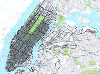
1       Introduction
It has been well documented that search frictions lead to less efficient outcomes.1 One particularly
salient reason for the existence of search frictions is that buyers and sellers are spatially distributed
across a city or region, so that meeting to trade requires costly transportation by one or both sides
of the market. When locations are fixed, say between households and potential employers, search
frictions arise from the added cost of travel associated with meeting. In some spatial settings,
however, every trade involves a future re-allocation of buyers or sellers. This is a prominent feature
of transportation markets, where every trade entails a vehicle moving from one place to another.
When transportation and search intersect, dynamic search externalities arise as each trip affects
the search frictions faced by future buyers and sellers at each destination. In this paper I study the
regulated taxicab industry in New York City, where a decentralized search process and a uniform
tariff leads to distortions in the intra-daily equilibrium spatial patterns of supply and demand. I
ask how much spatial misallocation is induced by search externalities in this setting and to what
extent simple changes to pricing regulations can enhance allocative efficiency over time.
    The taxicab industry is a critical component of the transportation infrastructure in large urban
areas, generating about $23 billion in annual revenues. New York City has long been the largest
taxicab market in the United States, accounting for about 25% of national industry revenues in
2013.2 In New York and many other cities, the taxi market is distinguished from other public
transit options by a lack of centralized control; taxi drivers do not service established routes or
coordinate search behavior. Instead, drivers search for passengers and, once matched, move them
to destinations. Since different types of trips are demanded in different areas of the city, how taxi
drivers search for passengers directly impacts the subsequent availability of service across the city.
These movements of capacity give rise to equilibrium patterns that can leave some areas with little
to no service while in other areas empty taxis will wait in long queues for passengers.
    In this paper, I model taxi drivers’ location choices in a dynamic spatial search framework in
which vacant drivers choose where to locate given both the time-of-day pattern of trip demand as
well as the distribution of rival taxi drivers throughout the day. While the spatial search process
under current regulations often generates mis-allocation across locations, I also model frictions
within each location to account for a block-by-block search process within small windows of time.

    1
      Models of search and equilibrium have been widely studied. Since the pioneering work of Diamond (1981,
1982a,b), Mortensen (1982a,b) and Pissarides (1984, 1985), the search and matching literature has focused on the
role of search frictions in impeding the efficient clearing of markets. The search and matching literature examines
many markets where central or standardized exchange is not possible, including labor markets (e.g., Rogerson, Shimer,
and Wright (2005)), marriage markets (e.g., Mortensen (1988)), monetary exchange (e.g., Kiyotaki and Wright (1989,
1993)), and financial markets (e.g., Duffie, Gârleanu, and Pedersen (2002, 2005)).
    2
      This value is based on my own calculation combining data from the NYC Taxi and Limousine Commission and
a national industry report Brennan (2014).

                                                         2
I show that spatial frictions are largely attributable to inefficient pricing, as tariff-based prices
fail to account for driver opportunity costs and the heterogeneity in consumer surplus that is not
internalized by drivers. To empirically analyze this model, I use data from the New York City
Taxi and Limousine Commission (TLC), which provides trip details including the time, location,
and fare paid for all 27 million taxi rides in New York between August and September of 2012.
Using TLC data together with a model of taxi search and matching, I estimate the spatial and
intra-daily distribution of supply and demand in equilibrium. Importantly, the data only reveal
matches made between taxis and customers as a consequence of search activity, but do not show
underlying supply or demand; I therefore cannot observe the locations of vacant taxis or the number
of customers who want a ride in different areas of the city. Because these objects are necessary
for measuring search frictions and welfare in the market, I develop an estimation strategy using
the dynamic spatial equilibrium model together with a local matching function. I show that the
observed distribution of taxi-passenger matches is sufficient to solve for drivers’ policy functions
and compute the equilibrium distribution of vacant taxis without direct knowledge of demand. I
then invert each local matching function to recover the implied distribution of customer demand
up to an efficiency parameter. Finally I estimate matching efficiency using moments related to the
variance of matches across days of the month.
    I use this model to evaluate welfare and search frictions in the New York taxi market. Baseline
estimates of welfare indicate that the New York taxi industry generates $2.2 million in consumer
surplus and $3.4 million in taxi driver variable profits during each 9-hour day-shift and across 216
thousand taxi-passenger matches, implying a combined surplus of about $25 per trip. Despite these
surpluses, however, there are on average 53 thousand failed customer searches per day and 5,756
vacant drivers at any point in the day. To what extent can a more sophisticated pricing policy
mitigate these costs by better allocating available supply to demand? By simulating market equi-
librium over nearly one million potential pricing rules, I am able to solve for a dynamically optimal
flexible fare structure and show that a flexible tariff that changes with time-of-day can provide up
to a 21% increase in consumer welfare and a 10% improvement in taxi utilization. These results
utilize an estimated demand system that incorporates an elasticity of waiting time calibrated from
recent work.3 Alternative policies offering flexible tariffs by location and distance yield slightly
smaller benefits to consumers in favor of driver profits and higher utilization rates, but all of the
counterfactual policies tested offer unambiguous benefits to both sides of the market even after
accounting for search and matching frictions. I contrast these results with a counterfactual sim-
ulation of ride-sharing technology that offers frictionless within-location matching, and show that
optimal pricing policies can produce nearly the same number of trips as the matching technology

   3
     c.f. Frechette, Lizzeri, and Salz (2019), Buchholz, Doval, Kastl, Matejka, and Salz (2019). Data limitations in
this setting prevent recovering waiting time elasticity directly.

                                                         3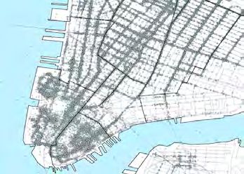
alone and deliver about 60% of the welfare gains.

Related Literature

This paper integrates ideas from the search and matching literature with empirical industry dy-
namics. The key component is a model of dynamic spatial choices that adapts elements from
Lagos (2000). Lagos (2000) studies endogenous search frictions using a stylized environment of taxi
search and competition. His model predicts how meeting probabilities adjust to clear the market
and how misallocation can occur as an equilibrium outcome. Lagos (2003) uses the Lagos (2000)
model to empirically analyze the effect of taxi fares and medallion counts on matching rates and
medallion prices in Manhattan. I draw elements from the Lagos search model, but make several
changes to reflect the real-world search and matching process. Specifically, I add non-stationary
dynamics, a more realistic and flexible spatial structure, stochastic and price-sensitive demand,
fuel costs, and heterogeneity in the matching process across different locations. Further, I build a
tractable framework for the empirical analysis of dynamic spatial equilibrium by providing tools for
estimating and identifying the model. I also model a static, localized market clearing process via
an aggregate matching function. Hall (1979) introduces the aggregate matching function concept,
using the urn-ball specification adapted in this paper.4 In recent work Brancaccio, Kalouptsidi,
and Papageorgiou (2019a,b) study the estimation and identification of matching functions in spatial
settings and apply a related search model to study endogenous trade costs in the bulk shipping
industry.5
    I also draw on literature for estimating dynamic models in the tradition of Hopenhayn (1992)
and Ericson and Pakes (1995), which characterize Markov-perfect equilibria in entry, exit, and
investment choices given some uncertainty in the evolution of the states of firms and their com-
petitors. Here, each taxi operates as a firm that is optimizing where to search in a city. The
state variable is the distribution of taxi locations. To facilitate computation, I make a large-market
assumption that both taxi drivers and customers are non-atomic. As in Hopenhayn (1992) this
allows me to compute deterministic state transitions without integrating over a high-dimensional
space of states and future periods. The mass of customers in each location varies from day to day
in each location and period. Drivers do not condition on these shocks, which I assume are not
observed by individual drivers, but rather the expectation of consumer demand. The equilibrium is
therefore similar to an Oblivious Equilibrium (Weintraub, Benkard, and Van Roy (2008b)) in which
drivers form their policies with respect to averages taken across many days in the market. This
    4
      Mortensen (1986), Mortensen and Pissarides (1999) and Rogerson, Shimer, and Wright (2005) survey the labor-
search literature and the implementation of aggregate matching functions.
    5
      There is also a literature in empirical industrial organization which studies the allocative distortions induced by
search frictions in different industries. This includes work on airline parts (Gavazza (2011) and mortgages (Allen,
Clark, and Houde (2014)).

                                                           4
notion is also similar to an Experience-Based Equilibrium (Fershtman and Pakes (2012)) in which
firms’ information set is restricted and agents condition their strategies on repeated experiences
with market outcomes.6
This is the first empirical analysis of pricing and welfare in a taxi market and the first to study
how price regulations impact the spatial allocation of service. A related study is Frechette, Lizzeri,
and Salz (2019), which models the dynamic entry game among taxi drivers to ask how customer
waiting times and welfare are impacted by medallion regulations and dispatch technology. Similar
to my paper, Frechette, Lizzeri, and Salz (2019) study the effect of regulations on search frictions
and welfare. The key difference is that they focus on the labor supply decision rather than the
spatial location decision.7 Though these research questions and approaches differ substantially,
they lead to similar predictions when comparing similar counterfactuals.
There is a recent literature on the benefits of dynamic pricing for ride-hail services (e.g., Hall,
Kendrick, and Nosko (2015), Castillo, Knoepfle, and Weyl (2017), Castillo (2019)). This paper also
highlights the impact of pricing on efficiency, but with two distinct differences. First, I focus on
posted tariffs instead of real-time price adjustment. Posted tariffs are a feature of both traditional
taxis and ride-hail services that affect the search behavior of taxi drivers. Second, I explicitly model
the influence of prices on the dynamic path of supply and demand. I use this model to show how
prices can be configured to induce efficient allocations of supply and demand while accounting for
the flow of reallocated of cabs due to passenger trips.
Finally, a diverse literature addresses whether taxi regulation is necessary at all. In this lit-
erature, both the theoretical and empirical findings offer mixed evidence. These studies point to
regulation’s ability to reduce transaction costs (Gallick and Sisk (1987)), prevent localized monop-
olies (Cairns and Liston-Heyes (1996)), correct for negative externalities (Schrieber (1975)), and
establish efficient quantities of vacant cabs (Flath (2006)). Other authors assert that regulations
restricted quantities and led to higher prices (Winston and Shirley (1998)) and that low sunk- and
fixed-costs in this industry are sufficient to support competition (Häckner and Nyberg (1995)). My
paper shows how existing regulatory levers are inefficient due to adverse static and dynamic con-
sequences of mis-pricing, and that a better implementation of posted tariffs leads to more efficient
spatial allocations and higher utilization.
6
This approach also relates to auction models with many bidders (e.g., Hong and Shum (2010)) and as an empirical
exercise in studying non-stationary firm dynamics (e.g., Weintraub, Benkard, Jeziorski, and Van Roy (2008a), Melitz
and James (2007)).
7
There is an additional body of literature on taxi drivers’ labor supply choices, including Camerer, Babcock,
Loewenstein, and Thaler (1997), Farber (2005, 2008), Crawford and Meng (2011), and Thakral and Tô (2017). These
studies investigate the labor-leisure tradeoff for drivers. They ask how taxi drivers’ labor supply is determined and
to what extent it is driven by daily wage targets and other factors. Buchholz, Shum, and Xu (2017) estimate a
dynamic labor supply model of taxi drivers to show that behavior consistent with dynamic optimization may appear
as a behavioral bias in a static setting.
5In section 2 I detail taxi industry characteristics relating to search, regulation, and spatial
sorting, as well as a description of the data. In section 3 I present a dynamic model of taxi search
and matching. Section 4 outlines my empirical strategy for computing equilibrium and estimating
model parameters. I present my results in section 5 and an analysis of counterfactual policies in
section 6. Section 7 concludes.
2 Market Overview and Data
2.1 Regulatory Environment
As with nearly all major urban taxi markets, the New York taxi industry is highly regulated. Two
regulations imposed by the New York Taxi and Limousine Commission (TLC) directly impact
market function and efficiency. The first is a fixed two-part tariff fare pricing structure, where
fares are based on a one-time flag-drop fee and a distance-based fee. Except for separate fares for
some airport trips, this fare structure does not depend on location. Except for an evening flat-rate
surcharge, fares do not depend on time of day. The second type of regulation is entry restrictions
imposed via a limit on the number of legal taxis that can operate. This is implemented by requiring
drivers to hold a “medallion” or permit, the supply of which is capped (Schaller (2007)).8 Medallion
cabs can only be hailed from the street and are not authorized to conduct pre-arranged pick-ups,
a service exclusively granted to separately licensed livery cars.
In recent years, several ride-hail firms including Uber and Lyft have entered the taxi industry
including the New York market. These firms operate a mobile platform to match customers with
cabs, greatly reducing frictions associated with taxi search and availability. The precipitous expan-
sion and popularity of ride-hail suggests there are large benefits associated with both the reduced
search costs and more flexible pricing compared with traditional taxi markets. Another potential
reason for this expansion is that taxi regulations are often at odds with this new wave of technology-
centered entrants. These firms tend to enjoy much less stringent entry restrictions than the more
regulated incumbents, leading to a variety of legal disputes as stakeholders in the traditional taxi
business absorb losses.9 These are high stakes disputes, and they highlight the need for analysis
surrounding the effects of these new entrants. My paper aims to understand how regulation and
matching technology impact the equilibrium spatial allocations of supply and demand as well as
the corresponding impact on market welfare and efficiency.10
8
These licenses are tradable, and the fact that they tend to have positive value, sometimes in excess of one million
dollars, implies that this quantity cap is binding and below the quantity that would be supplied in an unrestricted
equilibrium.
9
See, e.g.,
forbes.com/sites/ellenhuet/2015/06/19/could-a-legal-ruling-instantly-wipe-out-uber-not-so-fast/.
10
The spatial availability of taxis is of evident concern to municipal regulators around the country: a number of
62.2 Data
In 2009, the New York TLC initiated the Taxi Passenger Enhancement Project, which mandated
the use of upgraded metering and information technology in all New York medallion cabs. The
technology includes the automated data collection of taxi trip and fare information. I use TLC
trip data from all New York City medallion cab rides given from August 1, 2012 to September
30, 2012. An observation consists of information related to a single cab ride. Data include the
exact time, date and GPS coordinates of pickup and drop-off, trip distance, and trip time length
for approximately 27 million rides.12 New York cabs typically operate in two separate shifts of
9-12 hours each, with a mandatory shift change between 4–5pm. I focus on the weekday, day-shift
period of 7am until 4pm and I assume all drivers stop working at 4pm.
Due to New York rules governing pre-arranged trips, the TLC data only record rides originating
from street-hails. This provides an ideal setting for analyzing taxi search behavior since all observed
rides are obtained through search. Table 1 provides summary facts for this data set. I provide
additional monthly-level statistics in Appendix A.3.
Most of the time, New York taxis operate in Manhattan. When not providing rides within
Manhattan, the most common origins and destinations are New York’s two city airports, LaGuardia
(LGA) and John F. Kennedy (JFK). At the airports taxis form queues and wait in line for next
available passengers. Table 2 provides statistics related to the frequency and revenue share of trips
between Manhattan, the two city airports, and elsewhere.
Uber began operating in New York City in 2011, but service was minimal. In an October 2012
interview, the CEO reported that 160 drivers had provided trips in the city since the company’s
entry into New Yotk.13 This represents about 1% of licensed yellow cab drivers, and likely much
less in trip volume as these drivers were not necessarily operating consistently throughout the prior
year.
cities have introduced policies to control the spatial dimension of service. For example, in the wake of criticism over the
availability of taxis in certain areas, New York City issued licenses for 6,000 additional medallion taxis in 2013 with
special restrictions on the spatial areas they may service (See, e.g., cityroom.blogs.nytimes.com/2013/11/14/new-
york-today-cabs-of-a-different-color/). Specifically, these green-painted “Boro Taxis” are only permitted to pick up
passengers in the boroughs outside of Manhattan.11 Though the city’s traditional yellow taxis have always been
able to operate in these areas, it’s apparent that service was scarce enough relative to demand that city regulators
intervened by creating the Boro Taxi service. This intervention highlights the potential discord between regulated
prices and the location choices made by taxi drivers.
12
Using this information together with geocoded coordinates, we might learn for example that cab medallion 1602
(a sample cab medallion, as the TLC data are anonymized) picks up a passenger at the corner of Bowery and Canal
at 2:17pm of August 3rd, 2012, and then drives that passenger for 2.9 miles and drops her off at Park Ave and W.
42nd St. at 2:39pm, with a fare of $9.63, flat tax of $0.50, and no time-of-day surcharge or tolls, for a total cost of
$10.13. Cab 1602 does not show up again in the data until his next passenger is contacted.
13
Source: https://www.cnet.com/news/uber-quietly-puts-an-end-to-nyc-taxi-service/.
7Table 1: Taxi Trip and Fare Summary Statistics
Sample Rate Type Variable Obs. 10%ile Mean 90%ile S.D.
Total Fare ($) 27,475,614 4.50 9.51 16.00 5.57
Dist. Fare ($) 27,475,621 1.50 5.59 12.00 6.14
Standard
Flag Fare ($) 27,475,621 2.50 2.83 3.50 0.36
Fares
Distance (mi.) 27,475,621 0.82 2.70 6.00 2.74
All Data
Trip Time (min.) 27,475,621 4.00 12.04 22.52 8.23
Total Fare ($) 491,689 45 48.32 52 3.58
JFK Fares Distance (mi.) 491,689 3.02 16.25 20.58 5.95
Trip Time (min.) 491,689 22.75 39.49 60.00 17.33
Total Fare ($) 8,164,678 4.50 10.17 17.70 6.42
Dist. Fare ($) 8,122,794 1.20 4.66 9.60 5.33
Standard
Weekdays, Flag Fare ($) 8,122,794 2.50 2.5 2.5 0
Fares
Day-Shift, Distance (mi.) 8,122,794 0.71 2.28 4.67 2.37
Manhattan Trip Time (min.) 8,122,794 4.00 12.74 23.8 8.49
& Boro. Total Fare ($) 171,223 45.00 48.28 52.00 3.60
JFK Fares Distance (mi.) 171,223 2.00 16.14 20.91 6.09
Trip Time (min.) 171,223 26.18 45.65 67.00 19.16
Taxi trip and fare data come from the New York Taxi and Limousine Commission (TLC). This table provides statistics
related to individual taxi trips taken in New York City between August 1, 2012 and September 30, 2012 for two fare
types. The first is the standard metered fare (TLC rate code 1), in which standard fares apply, representing 98.1% of
the data. The second is a trip to or from JFK airport (TLC rate code 2). Total Fare and Distance data are reported
for each ride in the dataset. The two main fare components are a distance-based fare and a flag-drop fare. I predict
these constituent parts of total fare using the prevailing fare structure on the day of travel and the distance travelled,
though they are not separately reported either from each other or from waiting costs. Flag fare calculations include
time-of-day surcharges. Any remaining fare is due to a charge for idling time. The first set of statistics corresponds
to the full sample of all New York taxis rides across the two months, and the second set relates to the smaller sample
used in my analysis: weekdays, day-shift trips occurring within the space described in Figure 1.
2.3 Discretizing time and space
To analyze time and geography, I discretize time and space across the weekday, day-shift hours in
this market. Time is divided into five minutes periods. I divide space into 39 distinct areas that
are linked to observed GPS points of origin and destination for each taxi trip. These locations
represent 98% of all taxi ride originations, and I depict them in Figure 1. The average observed
travel time from one location to a neighboring location is 2 minutes, 45 seconds, or about one-half
of a five-minute period. This suggests that the 5-minute period is reasonably well-suited to this
geographic partitioning. For additional details on location selection and construction see Appendix
A.2.
I further denote five regions as disjoint subsets of all 39 locations. I depict regions as shaded
sections of Figure 1. Each region is characterized by a unique mix of geographical features and
8Table 2: Taxi Trips and Revenues by Area
Time Place Obs. Mean Fare Trip Share Rev. Share
Intra-Manhattan Trips 24,835,103 $9.28 89% 73%
All Times Airport Trips 1,568,699 $33.77 6% 17%
Other Trips 1,563,501 $19.83 6% 10%
Intra-Manhattan Trips 7,813,226 $9.33 91% 76%
Weekdays,
Airport Trips 503,711 $34.80 6% 18%
Day-shift
Other Trips 270,883 $19.62 3% 6%
Taxi trip and fare data come from New York Taxi and Limousine Commission (TLC). This table provides statistics
related to the locations of taxi trips taken in New York City between August 1, 2012 and September 30, 2012.
Intra-Manhattan denotes trips that begin and end within Manhattan, Airport Trips are trips with either an origin or
destination at either LaGuardia or JFK airport, and Other Trips captures all other origins and destinations within
New York City. Statistics are reported for all times as well as for the day-shift period of a weekday, from 6am until
4pm. I focus on weekday day-shifts in my analysis.
transit infrastructure. I will estimate the efficiency of search for each of these five regions. Region
I is lower Manhattan, an older part of the city where streets follow irregular patterns, and where
numerous bridges, tunnels and ferries connect to nearby boroughs and New Jersey. Region II is
midtown Manhattan, with fewer traffic connections away from the island, but denser centers of
activity including the major transit hubs Penn Station and Grand Central Station. Region III is
uptown Manhattan, where streets follow a regular grid pattern, but are longer and more spread
out. Few bridges, tunnels or stations offer direct connections to other boroughs. Region IV is the
large area encompassing Brooklyn and Queens. Region V consists of the two airports, John F.
Kennedy (JFK) and LaGuardia (LGA).
Table 3 summarizes how cabs move around space. Panel (a) aggregates all passenger trips into
Regions and all times of day to display the density of employed-taxi transitions between regions.
This matrix represents customer preferences for travel. At the end of a trip, taxis become vacant
in these new regions. Panel (b) displays the observed location of a matched taxi, at the start of a
ride, conditional on the last observed location of the same taxi, at the previous drop-off location.
Thus Panel (b) reveals the transition of vacant cabs, though not accounting for period-by-period
choices – only the eventual location of the next pickup. As I will show, an equilibrium estimate of
drivers’ period-by-period spatial choices closely mirrors the pattern of Panel (b), but with higher
frequency weights put on same-location transitions. The difference occurs because drivers search
on average for 2.5 periods before finding a passenger. The ride-to-ride transitions are therefore
more dispersed.
9Locations
and Regions
Region I
Region II
Region III
Region IV
Region V
Water/Rivers
Locations
LGA Airport
JFK Airport
Figure 1: 39-Location Map of New York City
Each of the outlined sections of Manhattan is one of the 39 locations indexed by i in my model. I create locations
by aggregating census-tract boundaries, which broadly follow major thoroughfare divisions. I compute the expected
travel time and distance between these locations separately for each origin and destination pair as the average of
all observations within each ij cell. Each shaded section depicts a region r, indicated with Roman numerals I–V.
Regions are characterized by similarities in transit infrastructure, road layouts, and zoning.
2.4 Evidence of Frictions
Search frictions occur when drivers cannot locate passengers even though supply and demand
coexist at the same point in time. Frictions in this market manifest as waiting time experienced by
drivers looking for a passenger.14 The TLC data provide evidence of search frictions for drivers that
vary across space and time of day. Using driver ID together with the time of pick-up and drop-off,
I compute the waiting time between trips. The mean waiting time for different trips is displayed
in Figure 2. Panel (a) shows the probability that a driver will find a passenger in each five-minute
period, as well as the expected waiting time to find a passenger in 10-minute units (i.e., a value of
0.5 equals 5 minutes). There is substantial intra-day variation in search times, with the best times
of day for finding passengers around 9am to 4pm, with average wait times around six minutes and
14
In a discrete-time sense, this means that after some interval of time some taxis will remain empty despite the
presence of demand somewhere else in the market.
10Table 3: Observed Pickup and Drop-off Activity by Region
Destination Destination
Region I Region II Region III Region IV Region V Region I Region II Region III Region IV Region V
Region I 0.3800 0.5005 0.0719 0.0215 0.0262 Region I 0.7625 0.1831 0.0286 0.0105 0.0154
Region II 0.1590 0.6287 0.1681 0.0094 0.0348 Region II 0.0613 0.7747 0.1409 0.0074 0.0157
Origin
Origin
Region III 0.0526 0.3770 0.5469 0.0061 0.0174 Region III 0.0143 0.1309 0.8340 0.0072 0.0136
Region IV 0.1905 0.2706 0.1067 0.3866 0.0456 Region IV 0.2213 0.1172 0.1488 0.3714 0.1414
Region V 0.1404 0.5417 0.1504 0.1095 0.0581 Region V 0.0621 0.1305 0.1861 0.0907 0.5306
(a) Passenger Trips (b) Vacant Transitions
This table summarizes transitions in the TLC data. Data in the table are aggregated to the regions from Figure 1.
Panel (a) depicts the transition density of taxi-passenger matches and Panel (b) depicts the transition of vacant taxis
between each drop-off and the same driver’s subsequent pickup.
five-minute finding rates around 50%. The worst times are in early morning and mid-day, when
average wait times are nearly 10 minutes and finding rates fall as low as 25%. Panel (b) shows
the same driver match probabilities and waiting times by the 37 non-airport locations, taken as an
average from 7am-4pm across all weekdays of the month. Again there is heterogeneity across space,
with relatively higher match probabilities and lower waiting times in lower Manhattan (1–8) and
Midtown (9–18), declining match probabilities in upper Manhattan (19–34), and even lower match
probabilities in Brooklyn (35–37).15 In aggregate, drivers spend about 47% of their time vacant
during the sample period of weekdays during the day-shift. This suggests that among 11,500 active
drivers, an average of 5,405 are vacant at any time.
Figure 2 provides a snapshot of the frictions faced by drivers by time-of-day and neighborhood.
The data do not reveal the frictions faced by customers; it is impossible to tell how long a customer
has been waiting before pick-up, and it is similarly not possible to tell if a customer arrived to
search for a taxi and gave up.
15
There is additional evidence that drivers often relocate to find passengers: 61.3% of trips begin in a different
neighborhood from the neighborhood where drivers last dropped off a passenger. This suggests that there are spatial
search frictions for drivers, as finding a customer requires relocation.
11Match Probability
5-min Match Probability
0.6
1
Mean Wait times (10-min units)
0.4
0.8
0.2
0 5 10 15 20 25 30 35
0.6
Mean Waiting Time (Min.)
0.4 10
0.2
5
0 5 10 15 20 25 30 35
7a 8a 9a 10a 11a 12p 1p 2p 3p 4p Locations 1 to 37
Figure 2: Taxi wait times and match probabilities by time-of-day and location
TLC Data from August 2012, Monday–Friday from 7am until 4pm, within regions indicated on Figure 1. Left Panel:
Each series shows taxi drivers’ five-minute probability of finding a customer and mean waiting times, averaged across
all drivers and all weekdays. Dotted lines depict 25th and 75th percentiles. Right Panel: Each bar shows driver
waiting times and matching probabilities by location of drivers’ last drop-off. Manhattan locations follow a roughly
South-to-North trajectory from index 1–34. Brooklyn locations are indexed 35–36. Queens is location 37.
3 Model
A city is a network of L nodes called “locations”, connected by a set of routes. A location can be
thought of as a spatial area within the city.16 Time within a day is divided into discrete intervals
with a finite horizon, where t ∈ {1, ..., T }. At time t = 1 the work day begins; at t = T it ends.
Model agents are vacant taxi drivers who search for customers within a location i ∈ {1, ..., L}. When
taxis find passengers, they drive them from origin location i to a destination location j ∈ {1, ..., L}.
Denote vit ∈ R as a measure of vacant taxis and denote uti ∈ R as a measure of customers looking for
a taxi in each location at each time. The total numbver of taxis in the city is given by i vit = v̄ for
P
all t. The distance between each location is given by δij and the travel time between each location
is given by τij .
My model has four basic ingredients. First, there is a demand system that describes, for every
neighborhood pair ij, how many customers will arrive to the market to search for a taxi as a
function of the price of service along that route. Second, there is a payoff vector associated with
every route that taxis service. Payoffs include the revenues from each ride minus a service cost
due to fuel expenses. Third, there is a model of period-by-period market clearing. Here I use an
aggregate matching function to map supply and demand into match probabilities, which adjust
16
e.g., a series of blocks bounded by busy thoroughfares, different neighborhoods, etc.
12payoffs depending on the relative quantities of taxis and customers.17 Finally, I combine these
components in a dynamic model of location choice. In this model vacant drivers make period-by-
period location choices accounting for the expected match probabilities and payoffs associated with
future locations. These four ingredients are presented in more detail below.
3.1 Demand
In each location i at time t, the measure of customers that wish to move to a new location, uti , is
drawn from a Poisson distribution with parameter λti . Moreover, λti is a sum of Poisson parameters
λti = j λtij (Pij ), where λtij (Pij ) represents the destination-j-specific Poisson arrival of customers
P
in location i at time t. The parameters λtij are functions of the price of a taxi ride between i and j,
Pij . Denote the probability that a customer in i wants to travel to location j ∈ {1, ..., L} at time t
by Mijt , so that λtij (Pij ) = Mijt · λti (P), where P is a vector of prices between all locations.
I assume that taxi drivers face a constant-elasticity demand curve. Demand depends on the
origin and destination of the trip, its price, and the time of day. Price elasticities depend on whether
the trip involves an airport (a binary index denoted by a) and the distance of the trip (indexed by
discrete categories s). Taxi demand takes the form:
ln(λtij (Pij )) = α0,i,t,s,a + α1,s,a ln(Pij ) + ηi,t,s,a . (1)
In addition, I assume that customers demand taxi services for one period. After this period,
consumers use a different method of transit.18
Waiting Time I do not observe customer waiting time, but it may be an important determinant
of demand for taxi rides. To identify the price elasticity of demand in this specific exercise, I
provide evidence that waiting time is negligible or of second-order importance. There are two
primary reasons for this. First, since the estimation of demand parameters λtij does not require
knowledge of waiting time or price elasticities, I compute a measure of waiting time via customer
match probabilities.19 The September price change, later used to identify price elasticities, leads
to an estimated average waiting time change of approximately 21 seconds. Further, the limited
empirical evidence for waiting time elasticities suggests that it should be relatively small. Frechette,
17
Note that in a setting of ride-hail, in which prices adjust to neighborhood market conditions, we might instead
recast this model as one of localized price formation instead of search frictions.
18
In the empirical analysis to follow, I define one period as five minutes. In the context of New York City, there
are plenty of alternative transport options, and this assumption suggests that customers will choose to travel via one
of these alternatives upon failing to find a taxi.
19
This estimate is premised on the assumption that consumer search takes at most five minutes, after which
consumers exit the market. Consumers find a match with probability qit = mti /λti where mtij is the observed matches
in each i, t cell. I then compute a measure of expected waiting time (in units of minutes) as 5 · (1 − qit ) assuming any
matches are made instantaneously.
13Lizzeri, and Salz (2019) estimate waiting time elasticity of demand to be about -1.2, while Buchholz,
Doval, Kastl, Matejka, and Salz (2019) estimate average waiting time elasticity in a large European
taxi market to be -0.66. In the European setting, authors estimate a convex relationship between
cost of waiting and length of waiting, which suggests that small waiting times have an even smaller
impact on demand than would be suggested by the average elasticity. In counterfactuals, however,
I study changes to pricing policies that may be large enough to meaningfully impact waiting times.
Therefore in all counterfactuals I implement a waiting time elasticity calibrated to -1.0 and allow
demand to adjust accordingly.
3.2 Revenue and Costs
Taxis earn revenue from giving rides. At the end of each ride, the taxi driver is paid according to
the fare structure. The fare structure is defined as follows: b is the one-time flag-drop fare and π
is the distance-based fare, with the distance δij between locations i and j. The total fare revenue
earned by providing a ride from i to j is b + πδij .
Drivers have two sources of costs. First, there is a fixed daily fee for leasing the taxi and
medallion license (or a financing cost for drivers who own their own medallion). Second there are
per-mile fuel costs, which I denote as cij . On any particular day a driver is working, medallion
leasing costs for that day are sunk and therefore independent of the driver’s search choices. Since
my analysis holds fixed the entry decisions of taxis, I ignore these costs in the model and focus on
drivers’ optimization while working.
The net revenue of any passenger ride is given by
Πij = b + πδij − cij . (2)
This profit function sums the total fare revenue earned net of fuel costs in providing a trip from
location i to j.
3.3 Searching and Matching
At the start of each period, taxis search for passengers. The number of taxis in each location at
the start of the period is given by the sum of previously vacant taxis who have chosen location i to
search, plus the previously employed taxis who have dropped off a passenger in location i. This sum
is denoted as vit . I make the following assumptions about matching: (1) matches can only occur
among cabs and customers within the same location, (2) matches are randomly assigned between
taxis and customers, and (3) once a driver finds a customer, a match is made and the driver cannot
refuse a ride.20 The expected number of matches made in location i and time t is given by an
20
In New York, the TLC prohibits refusals, c.f. www.nyc.gov/html/tlc/html/rules/rules.shtml.
14passengers arrive taxis w/ passengers
with Poisson param. λti
expected matches =
mi (λti , vit ) (remaining customers wait
5-minutes and disappear)
match probability =
mi (·,·)
pti = vit
vacant taxis + taxis vacant taxis
dropping off passengers = vit
Figure 3: Flow of demand, matches, and vacancies within a location
This illustration depicts the sources of taxi arrivals and departures in location i at time t. At the beginning of a
period, all taxis conducting search in location i have either dropped off passengers or were searching from previous
periods. In expectation (given randomness in the mass of customers arriving each day), matches are determined by
mi (λti , vit ). At the end of the period, any employed taxis leave for various destinations and vacant taxis continue
searching.
aggregate matching function mi (λti , vit ). The ex-ante probability that a driver will find a customer
mi (λti ,vit )
is then given by pti = vit
. Figure 3 illustrates the within-period search and matching process.
3.3.1 A Model of Neighborhood Search
There are two types of locations, neighborhoods and airports. Neighborhoods comprise most of a
city; they are locations in which cabs drive around to search for passengers. Below I detail how
matches are formed in neighborhoods. The next subsection discusses airports.
When model locations are specified as spatial areas such as a neighborhood, search within this
area will exhibit search frictions even when block-by-block search is nearly frictionless. This design
echoes the setup of Lagos (2000) that allows search frictions to arise endogenously from driver
behavior. To model the search frictions within each location, I use an aggregate matching function
given by equation 3.21
λti
!
−
αr v t
m(λti , vit , αr ) = vit · 1−e i (3)
Equation 3 is a reduced-form model of intra-location matching. It can flexibly reproduce fric-
tions (i.e. such that m(λti , vit , αr ) < min(λti , vit )), the extent of which are controlled by the search
21
This function is derived from an urn-ball matching problem first formulated in Butters (1977) and Hall (1979).
While the original model characterizes matches from discrete (i.e., integer) inputs, my specification characterizes
urn-ball matching with a large number (or continuum) of inputs. See, e.g., Petrongolo and Pissarides (2001) and the
derivation in Appendix A.8.
15efficiency parameter αr > 0. All else equal, larger values of alpha generate fewer matches. r denotes
a region, or a subset of locations as described in section 2.3. αr is region-specific as it reflects the
difficulty of search within a region, such as the complexity of the street grid. These are physical
characteristics of a region which are assumed to be fixed across the day. I illustrate the aggregate
matching function and the role of αr in Figure 4.
Moreover, this equation is specified in terms of expected demand λti and not the daily draws uti .
It represents the expected number of matches produced in a location-time with demand parameter
λti and vacant taxi supply vit . This is the relevant object from the perspective of taxi drivers’
location optimization problem. From now on I denote mi (λti , vit ) = m(λti , vit , αr ) to be the location-
specific matching function, with the only difference across locations coming from the efficiency of
the region r containing location i. The probability of a match from a taxi driver’s perspective is
therefore given by
λti
!
mi (λti , vit ) −
αr v t
pi (λti , vit ) = = 1−e i . (4)
vit
,=0.5 ,=1.0 ,=1.5
100 80 100 100
35
20
Customer Arrivals (6)
Customer Arrivals (6)
Customer Arrivals (6)
80 65 80 50 80
20
20
60 60 60 35
50
35
5
40 40 40
5
35
5
20 20 20
20 20 20
5 5 5
20 40 60 80 100 20 40 60 80 100 20 40 60 80 100
Taxis (v) Taxis (v) Taxis (v)
Figure 4: Matching Efficiency and α
This figure shows contour plots of the matching function over three values of α. Contour levels depict the expected
number of matches produced in a given location when the level of taxis is v and the expected arrivals of customers
is λ, for each level of α.
3.3.2 Airport Queueing
At airports, taxis pull into one of multiple queues and wait for passengers to match with cabs at the
front of the queue.22 I assume there is some measure of congestion in the taxi lane, so that no more
22
In the data, rides involving one of the two major New York airports comprise roughly 6% of all taxi trips, and
16% of revenues.
16than v̄it cabs can clear the queue in each period. This condition prevents instantaneous clearing of
the taxi queue. The total number of matches is thus given by min{uti , wit }, where wit = min(v̄it , vit )
and where the total measure of cabs at the airport in each period is vit . From a taxi driver’s
perspective, airports represent match probabilities of one, but at the expense of time spent waiting
for the match. The more taxis there are in line, the more periods it will take to for a new driver
entering the queue to find a match.
3.4 Dynamic Model of Taxi Drivers’ Locations, Actions and Payoffs
A taxi driver’s behavior depends on his own private state (`ta , eta ) and the market state, S t . Specif-
ically a driver a’s own location at time t is given by `ta ∈ {1, ..., L}, and his employment status
(vacant or employed) is eta ∈ {0, 1}. Let mkij denote the set of ij matches occurring at starting time
k. The market state S t at time t is a measure of vacant taxis vit in each location i and a measure
of employed taxis mki,j that are in-transit between locations.23 Thus the market state at time t is
summarized by
S t = {{vit }i∈{1,...,L} , {mkij }i,j∈{1,...,L}2 ,kt+τij
plus continuation values Vj of being in location j after τij periods have elapsed. Therefore the
expected value of a trip is simply the value of a trip to each location j weighted by the probability
that a passenger picked-up in i chooses j as the destination, which is given by Mijt .24
At the end of the period, any cabs that remain vacant can choose to relocate or stay put to
begin a search for passengers in the next period. The set A(i) reflects the set of locations available
to vacant taxis and is limited to all adjacent locations in the city, where adjacency is defined as
locations that can be reached in one period or less. In addition, all trips to and from airports are
included in each choice set.
Vacant drivers choose to search next period in the location that maximizes total expected
t+τij
payoff as the sum of continuation values Vj (S), fuel costs cij and a contemporaneous and an
idiosyncratic shock εtja . εtja is a driver a-specific i.i.d. shock to the perceived value of search in
each alternative location j, which I assume to be drawn from a Type-I extreme value distribution.
This shock accounts for unobservable reasons that individual drivers may assign a slightly greater
value to one location than another. For example, traffic conditions and a taxi’s direction of travel
within a location may make it inconvenient to search anywhere but further along the road in the
same direction.25
Vacant drivers in location i move to location j ∗ by solving the last term in equation 6:
t+τij
j ∗ = arg max{Vj (S t+τij ) − cij + εja }. (7)
j
To compute the drivers’ strategies, I define the ex-ante choice-specific value function as Wit (ja , S t ),
which represents the net present value of payoffs conditional on taking action ja while in location
i, before εja is observed:
h i
t+τ
Wit (ja , S t ) = ES t+τija Vja ija (S t+τija ) − cija . (8)
Defining Wit allows for an expression of taxi drivers’ conditional choice probabilities: the prob-
ability that a driver in i will choose j ∈ A(i) conditional on reaching state S t , but before observing
εja , is given by
exp(Wit (ja , S t )/σε )
Pit [ja |S t ] = P t t
. (9)
k∈A(i) exp(Wi (jk , S )/σε )
This expression defines aggregate policy functions σit = {Pit [j|S t ]}j∈{1,...,L} as the probability of
optimal transition from an origin i to all destinations j conditional on future-period continuation
24 t
Note that Mij has superscript t because passenger preferences change throughout the day.
25
The terms εja also ensure that vacant taxis leaving one location will mix among several alternative locations
rather than moving to the same location, a feature broadly corroborated by data.
18values.
Time ends at period T . Continuation values beyond t = T are set to zero: Vit = 0 ∀t > T, ∀i.
Employed taxi drivers with arrival times beyond period T are assumed to finish en-route trips
before quitting.
3.5 Intraday timing
There is an exogenous initial distribution of vacant taxis labeled S 1 which is known to all drivers
and constant across each weekday. This distribution accounts for the early morning position of
taxis, all of which are assumed vacant at this time, as they leave from garages and arrive to the
search regions of the city. Vacant taxis conduct search at the start of each period t. At the end
of a period any newly employed taxis disappear from the stock of vacant cabs and earn revenue.
Vacant taxis earn no revenues but face continuation values associated with each possible move. In
the next period t + 1, the locations of vacant taxis are updated based on movement from both
previously vacant taxis who have relocated as well as any taxis dropping off passengers.
As detailed in the equilibrium description, I assume drivers are unaware of the i.i.d. demand
shocks in each location and time, and instead condition policies on long-run market averages (which
might, for example, be learned through experience). Since the expectation of a Poisson random
variable with parameter λ is also equal to λ, λti is the expected demand faced by taxi drivers.
Drivers form policies based on forecasting the following sequence of events:
1. Taxis are exogenously distributed each day according to S 1 .
2. mi (λ1i , vi1 ) taxis become employed with matched customers in each location.
3. The remaining λti − mi (λ1i , vi1 |αi ) unmatched customers leave the market.
4. The remaining vit − mi (λ1i , vi1 |αi ) vacant taxis choose a location to search in next period
according to policy functions.
5. Previously vacant and some previously employed taxis arrive in new locations, forming dis-
tribution S 2 .26
6. The process repeats from S 2 , S 3 , etc. until reaching S T .
26
Many hired taxis are in-transit for more than one period. Suppose hired taxis providing service from location i
to j will take 3 periods to complete the trip. Then only the taxis who were 1 period away at time t − 1 will arrive in
j in period t.
193.6 Transitions
Policy functions σit form a matrix of transition probabilities from origin i to all destinations j ∈ L.
Note that only vacant taxis transition according to these policies. Employed taxis will transition
according to a different matrix of transition probabilities given by Mit denoting the probability
that a matched customer in i will demand transit to any destination j ∈ L. Together, these two
transition processes generate a law of motion for the state variable S.
The transition kernel of employed taxis is given by ν(vet+1 |vet , M t , mt ) where vet is the distri-
bution of employed taxis across locations in period t, M t = {Mijt } for i, j = {1, ..., L} is the set of
transition probabilities of each matched passenger at time t and mt = {mi (λti , vit )} for i = {1, ..., L}
is the distribution of matches. ν specifies the expected distribution of all employed taxis ve , it over
locations in period t + 1.
Likewise, the transition kernel of vacant taxis is given by µ(vvt+1 |vvt , σ t ). As with ν, µ specifies
the expected t + 1 spatial distribution of period t vacant taxis, given the transitions generated from
policies σ t = {σit } for i = {1, ..., L}. The combined set of transitions forms an aggregate transition
kernel that defines the law-of-motion, given by Q(S t+1 |S t ) = ν(vet+1 |vet , M t , mt ) + µ(vvt+1 |vvt , σ t ).
I provide explicit formulas for the state transitions in Appendix A.5.
3.7 Equilibrium
Taxi drivers policies in a given period depend on the beliefs about the distribution of their com-
petitors, policies of competitors when vacant, expected demand across different neighborhoods and
the destination preferences of customers across neighborhoods. Beliefs over competitors’ policies
given the distribution of all vacant cabs allow taxi drivers to infer how the distribution of vacant
cabs at time t will update in future periods. Likewise, driver forecasts about demand and customer
destination preferences across neighborhoods allow drivers to infer how the distribution of matched
cabs and their movement will affect the future distribution of vacant cabs. The net transition of
taxis’ vacant capacity is denoted as Q̃ti .
Although drivers have knowledge of the Poisson demand parameters λti , I assume they do not
see actual draws uti , which are spread across multiple blocks within a location.27 Any successful or
unsuccessful match is attributed to a long-run probability of matching in each location and period
and there is no intra-day updating of beliefs based on whether the driver is matched or not.
Taxis optimize over where to locate when vacant. Since beliefs about the state and transitions
at time t summarize all relevant information about distribution of competition, taxis condition only
on beliefs over the current-period so that an optimal location choice at time t can be made using
time t − 1 information. This Markovian structure permits the following definition of equilibrium:
27
See Assumption 2 in Section 4.
20Definition Equilibrium is a sequence of state vectors S t , transition beliefs {Q̃ti } and policy
functions σit over each location i = {1, ..., L}, and an initial state Si0 ∀i such that:
(a) In each location i ∈ {1, ..., L}, at the start of each period, matches are made according to
equation 3 and are routed to new locations according to transition matrix M t . The aggregate
movement generates the employed taxi transition kernel ν(vet+1 |vet , M t , mt ) where vet is the
distribution of employed taxis across locations in period t and mt is the distribution of matches
across locations.
(b) In each location i ∈ {1, ..., L}, at the end of each period, vacant taxi drivers (indexed by a)
t (S t , Q̃t ) that (a) solves equation 7 and (b) derives expectations
follow a policy function σi,a i
under the assumption that the state transition is determined by transition kernel Q̃ti . The
aggregate movement generates the vacant taxi transition kernel µ(vvt+1 |vvt , σ̃ t , S t ) where vvt is
the distribution of vacant taxis in period t.
(c) State transitions are defined by the combined movement of vacant taxis and employed taxis,
defined by Q(S t+1 |S̃ t ) = ν(v t+1 |v t , M t , mt ) ∪ µ(v t+1 |v t , S˜t ).
e e v v
(d) Agents’ expectations are rational, so that transition beliefs are self-fulfilling given optimizing
behavior: Q̃ti = Qti for all i and t.
Proposition 3.1. The equilibrium defined above exists and is unique.
Proof. See Appendix A.6
Equilibrium delivers a distribution of vacant taxi drivers such that no one driver can systemati-
cally profit from an alternative policy: there is no feasible spatial arbitrage opportunity that would
make search more valuable (ex-ante) in any location other than the optimum one. Vacant taxis
are therefore clustered in locations with more profitable customers, but the associated profits are
offset by higher search frictions. One implication of this sorting pattern is that equilibrium value
functions are nearly identical across space in each time period. Moreover, equilibrium value func-
tions would equate across locations in each period if not for transportation costs in time and fuel,
preventing an equilibrium with perfect spatial arbitrage. See additional discussion and illustration
in Appendix A.9.
4 Empirical Strategy
To estimate model parameters I use each month of the New York TLC data and aggregate trip-
specific information into daily quantities related to customer transit preferences, trip times and
21trip distances for each weekday day-shift period. To form moments related to drivers’ beliefs and
payoffs I further average these daily quantities into monthly averages. When taxi drivers engage
in equilibrium search behavior, they incorporate these monthly averages into forecasts that enter
their continuation values. I present an estimation strategy below that is configured to (1) solve for
equilibrium and (2) use this equilibrium to recover parameters, both at a monthly-average level of
resolution. Below I detail these two main components of estimation.
4.1 Computing Equilibrium
The equilibrium location choices of vacant taxi drivers and their resulting spatial allocations must
be computed in order to estimate model parameters. I make the following assumptions about the
total supply of taxis and their information set.
Assumption 1 The total supply of cabs v̄ for each weekday day-shift during the period studied
is equal to 11,500.
Assumption 1 satisfies a requirement for an exogenous labor supply necessary to compute the
equilibrium level of vacant taxis across time and locations.28
Assumption 2 Taxi drivers have knowledge of the initial state vector S 1 and all model pa-
rameters including demand parameters {λti }. Drivers do not observe the specific draws from the
distributions of demand across time and locations.
Assumption 2 not only provides computational tractability, but also provides a behavioral model
that is motivated by drivers’ inability to observe supply or demand beyond the particular streets
they drive on in one period.
To solve for equilibrium I use a two-step procedure where in the first step the set of equilibrium
matches {mti } are non-parametrically estimated using trip data. I estimate matches by computing
the mean matches in each i, t cell for each day of the month. These moments contain all relevant
information needed for the second step, which solves the taxi drivers’ spatial equilibrium up to
σε . Equation (4) makes this second step explicit: the moments from the first step are the only
inputs to the value functions that contain information on demand. This step is the most involved
as it entails solving for non-stationary equilibrium value functions and policy functions given an
exogenous initial condition (i.e. the distribution of locations where drivers start their shift) and an
exogenous labor supply.
28
The number is data-driven; see Section A.4 for details.
22You can also read