In Search of Information: Use of Google Trends' Data to Narrow Information Gaps for Low-income Developing Countries$ - American Economic Association
←
→
Page content transcription
If your browser does not render page correctly, please read the page content below
In Search of Information: Use of Google Trends’ Data to Narrow
                 Information Gaps for Low-income Developing CountriesI

                                                  Futoshi Naritaa,∗, Rujun Yina
                    a International   Monetary Fund, 700 19th Street, NW, Washington, DC 20431, United States

    Abstract
    Timely data availability is a long-standing challenge in policy-making and analysis for low-income developing
    countries. This paper explores the use of Google Trends’ data to narrow such information gaps and finds
    that online search frequencies about a country significantly correlate with macroeconomic variables (e.g.,
    real GDP, inflation, capital flows), conditional on other covariates. The correlation with real GDP is stronger
    than that of nighttime lights, whereas the opposite is found for emerging market economies. The search
    frequencies also improve out-of-sample nowcasting performance albeit slightly, demonstrating their potential
    to facilitate timely assessments of economic conditions in low-income developing countries.
    Keywords: Google search volume index, Low-income developing countries, Nighttime lights, Nowcasting,
    Economic growth, Capital flows
    JEL: O11, O47, O57, E37, F17, F37

    1. Introduction

        Timely data availability in low-income developing countries (LIDCs) is a long-standing challenge to
    researchers and policy makers. LIDCs have more missing data and longer time lags in data release than
    more developed economies. For example, as of July 2018, official FDI data for 2017 are available only for less
5   than half of LIDCs, compared to 90 percent for advanced economies.1 A survey of the IMF staff indicates
    severer deficiencies in data quality and availability for low-income countries (Independent Evaluation Office,
    2016, Figure 2). The lack of reliable and timely information hampers real-time assessment of economic
    conditions and restricts the ability to set sound policies.
        Nontraditional data sources—so-called big data—have proven to be useful in providing operationally

       I Acknowledgment: We deeply thank Mamoon Saeed, Kei Moriya, and the Google Trends support team for their excellent

    technical support and Karina Chavez for her diligent editorial assistance. We also thank Sebastian Acevedo, Emre Alper,
    Claudia Berg, Alessandro Cantelmo, Rupa Duttagupta, Stefania Fabrizio, Rahul Giri, Wei Guo, Daniel Gurara, Roland Kpodar,
    Sandra Lizarazo Ruiz, Ali Mansoor, Marco Marini, Giovanni Melina, Machiko Narita, Neree Noumon, Chris Njuguna, Chris
    Papageorgiou, Saad Quayyum, Mahvash Qureshi, Alessandro Rebucci, Sidra Rehman, Sakina Shibuya, and the participants
    in the presentation at the IAAE 2019 Annual Conference and the seminars at the IMF for their thoughtful comments and
    suggestions. We are responsible for any remaining errors. This paper is part of a research project on macroeconomic policy
    in low-income countries supported by the U.K.’s Department for International Development (DFID, project ID: 60925, IATI
    Identifier: GB-1-202960). The views expressed in this paper are those of the authors and do not necessarily represent the views
    of the Internatinoal Monetary Fund (IMF), its Executive Board, IMF management, or the DFID.
       ∗ Corresponding author

         Email addresses: fnarita@imf.org (Futoshi Narita), yinrujunjoy@gmail.com (Rujun Yin)
       1 The calculation is based on the International Financial Statistics database (IMF, 2018b). A fraction of missing values

    for FDI data since 2000 is 22 percent for LIDCs, compared to 12 percent for all the other non-LIDC economies. See Table
    B.1 for the country groupings. Note that the situation has been improving, because of country authorities’ own efforts and
    international initiatives to address data gaps, including G-20’s Data Gaps Initiative (https://www.imf.org/en/Publications/
    SPROLLs/g20-data-gaps-initiative).

    Preprint submitted to Elsevier                                                                             December 31, 2019
10   valuable information in LIDCs.2 Satellite imagery data, such as nighttime lights, are used to measure
     economic growth and poverty in countries and sub-regions where data are scarce (Henderson et al., 2012;
     Jean et al., 2016; Engstrom et al., 2017). In Kenya, researchers analyze mobile phone call records to help
     combat malaria more effectively (Wesolowski et al., 2012). A sensor technology generates usage statistics to
     improve performance of water pumps in Kenya and Ethiopia (Thomas et al., 2018, Table B.1).
15       This paper explores the potential of Google’s search volume index (SVI)—a frequency of online search
     query submissions—to help narrow information gaps in LIDCs. Google’s SVI would contain fruitful informa-
     tion about individuals’ interests and attentions, considering the growing access to the Internet—especially,
     through mobile devices in developing countries—and Google’s global user share of over 90 percent (Stat-
     Counter, 2018). People may search for information online to make economic decisions or to look for some
20   developments in the economy. The SVI may capture these human behaviors in search of information, and
     that is the information potentially useful for economic analyses (see Appendix A.4, for discussion to for-
     malize this idea). The information search could be more relevant for cross-border activities—travel, trade,
     foreign investment—that may face larger information barriers than local activities, and thus, it could be
     particularly useful for analyses on LIDCs, where such external economic activities play a key role (IMF,
25   2015a). Timely availability of Google’s SVI is key in tackling information gaps due to the time lag in
     releasing official statistics in LIDCs.
         To the best of our knowledge, this is the first study to apply Google’s SVIs to a macroeconomic analysis
     on a comprehensive set of developing countries. The existing literature focuses on the use of Google’s
     SVI for more developed countries than LIDCs (Table 1). Following (Choi and Varian, 2012, a working
30   paper version was released in 2009), many researchers started to use Google’s SVI to forecast or nowcast
     socioeconomic indicators.3 The official statistical authorities and central banks have also adopted Google’s
     SVIs and other big data for policy-making, data compilation, and economic research. But, the efforts are still
     largely concentrated in advanced or frontier emerging economies (IMF, 2018d, Box 3), likely reflecting the
     fact that online searches are more prevalent in these countries. We argue, however, that useful information
35   on LIDCs may be able to be extracted from the online searches made in higher-income countries if these
     searches are about LIDCs. Our main analysis covers about 50 LIDCs (less than the total of 59 due to lack
     of macroeconomic data, while SVIs are available for all countries), and we also extend the analysis to about
     90 other emerging and developing economies.
         We find that Google’s SVI can provide useful information to enhance real-time monitoring of economic
40   conditions in LIDCs. We construct a panel data set of the SVI for each country by setting the country name
     as a search topic. And to be more granular, we further collect SVIs by category. For example, for Uganda,
     the SVI under the finance category increases if someone submits a query such as Uganda exchange rate, other
     things being equal. We choose five categories (finance; business and industrial; law and government; health;
     travel) and find in-sample significance of some of these SVIs in simple regression models of contemporaneous
45   forecasting (i.e., nowcasting) that predict macroeconomic variables, conditional on lagged covariates. The
     use of these SVIs also improves out-of-sample performance, albeit slightly, measured by the mean of squared
     forecasting errors, computed by recursive forecasting regressions.
         Using SVIs under various categories altogether seems to help disentangle positive and negative effects
     from the changes in individuals’ attentions to a country. SVIs may signal confounded offsetting effects and
50   it has been an issue in the application of the SVI (e.g., see Vozlyublennaia, 2014; page 18). In normal time,
     people may pay attention to a country if they are involved in some activities in the country, such as, searching
     for accommodations. This way, SVIs help identify positive effects on the country’s economy. However, people
     may also pay attention because of natural disasters, conflicts, epidemics, scandals, etc. These events are

        2 In contrast to traditional data that are compiled for specific purposes, big data are collected as a byproduct of other

     activities (Hammer et al., 2017). The United Nations Economic Commission for Europe (UNECE) provides classification of
     big data (UNECE, 2013). The Week @ the Beach Index proposed by Laframboise et al. (2014) is an example of the use of
     nontraditional data sources in economic analysis.
        3 Active areas of research include finance (predicting stock price and volatility, following a seminal paper of an “attention

     index” by Da et al., 2011); health (including the famous Google Flu Trend by Ginsberg et al., 2009, and its refinement by
     Lampos et al., 2015); tourism (forecasting tourist arrivals); sociology (measuring issue salience); and political science (voting
     behaviors). IMF (2015c, Figure 2) uses SVIs to illustrate tourism demand to Samoa.

                                                                    2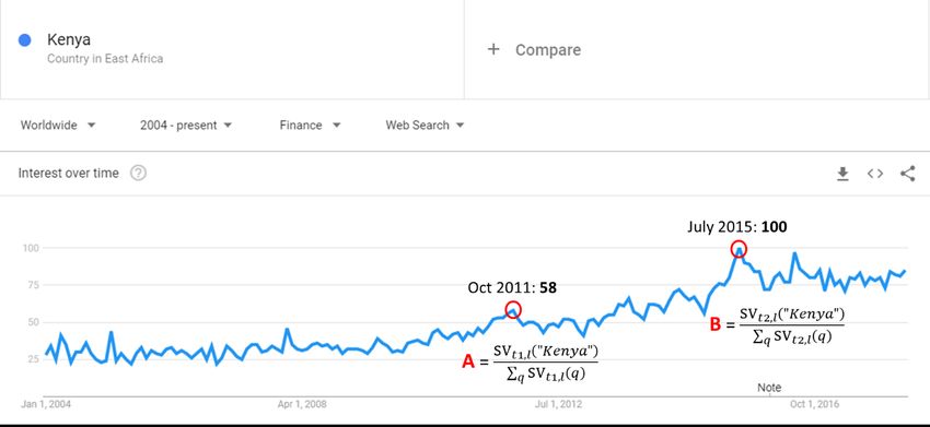
Table 1: Use of Google’s SVI in forecasting/nowcasting economic variables

Author (publication year)             Country under analysis            Variable to predict
Götz and Knetsch (2019)              Germany                           GDP
Ferrara and Simoni (2019)             Euro area                         GDP
Chamberlin (2010)                     United Kingdom                    Retail sales
Carrière-Swallow and Labbé (2013)   Chile                             Car sales
Barreira et al. (2013)                France, Italy, Portugal, Spain    Car sales
Askitas and Zimmermann (2009)         Germany                           Unemployment rate
Fondeur and Karamé (2013)            France                            Unemployment rate
Ross (2013)                           United Kingdom                    Unemployment rate
Reis et al. (2014)                    France, Italy                     Unemployment rate
Ferreira (2014)                       Portugal                          Unemployment rate
Chadwick and Sengül (2015)           Turkey                            Unemployment rate
Vicente et al. (2015)                 Spain                             Unemployment rate
Smith (2016)                          United Kingdom                    Unemployment rate
D’Amuri and Marcucci (2017)           United States                     Unemployment rate
Vosen and Schmidt (2011)              United States                     Consumption
Wu and Brynjolfsson (2015)            United States                     House price
Li et al. (2015b)                     China                             Consumer price index
Li et al. (2015a)                     United States                     Oil prices
Bangwayo-Skeete and Skeete (2015)     Caribbean countries               Tourist arrivals
Yang et al. (2015)                    China                             Tourist arrivals
Li et al. (2017)                      China                             Tourist arrivals
Artola et al. (2015)                  Spain                             Tourist arrivals
Siliverstovs and Wochner (2018)       Switzerland                       Tourist arrivals
Rivera (2016)                         Puerto Rico                       Hotel registrations
Da et al. (2011)                      United States                     Stock prices/returns
Joseph et al. (2011)                  United States                     Stock prices/returns
Preis et al. (2013)                   United States                     Stock prices/returns
Vozlyublennaia (2014)                 United States                     Stock prices/returns
Takeda and Wakao (2014)               Japan                             Stock prices/returns
Tantaopas et al. (2016)               Six AEs and four EMEs             Stock prices/returns
Adachi et al. (2017)                  Japan                             Stock prices/returns
Tang and Zhu (2017)                   United States                     Stock prices/returns
Welagedara et al. (2017)              United States                     Stock prices/returns
                                                                        Real estate investment
Yung and Nafar (2017)                 United States
                                                                        trusts’ (REITs) returns
Vlastakis and Markellos (2012)        United States                     Stock market volatility
Smith (2012)                          Eight AEs                         Stock market volatility
Aouadi et al. (2013)                  France                            Stock market volatility
Hamid and Heiden (2015)               United States                     Stock market volatility
Da et al. (2015)                      United States                     Stock market volatility
Dimpfl and Jank (2016)                United States                     Stock market volatility
Moussa et al. (2017)                  France                            Stock market volatility
Goddard et al. (2015)                 Five AEs                          Exchange rate volatility
Peltomäki et al. (2018)              25 EMEs                           Exchange rate volatility
Afkhami et al. (2017)                 United States                     Energy price volatility
Campos et al. (2017)                  United States                     Energy price volatility
                                                                        Nine macroeconomic
Koop and Onorante (2013)              United States
                                                                        indicators
 Source: Authors’ survey.

 Note: This list may not be exhaustive, and any omissions are purely incidental. See also Buono
 et al. (2017) for a broader survey on the use of nontraditional data in macroeconomic nowcasting.
 AEs: advanced economies; EMEs: emerging market economies.

                                               3
rather associated with negative effects on the economy. Combining SVIs under different categories may help
55 separate these offsetting effects, albeit not perfectly.4 We generally find that the business-and-industrial and
travel categories tend to be associated with positive effects, whereas the finance, law-and-government, and
health categories tend to indicate negative effects.
The SVIs show stronger correlation with real GDP than that of nighttime lights for LIDCs, while the
opposite is found for emerging market economies (EMEs). The significance of SVIs in the regressions for real
60 GDP shows a stark contrast with the results for nighttime lights extracted from satellite imagery (Henderson
et al., 2012), which lost significance once lagged covariates are included in the regressors. This is striking,
because nighttime lights are well accepted as a proxy to economic activity in the development literature.
For EMEs, however, nighttime lights significantly correlate with real GDP while SVIs are not as significant
as in the case of LIDCs. This contrasting finding may indicate some structural differences between LIDCs
65 and EMEs.
In addition to these new empirical findings, this paper also contributes to the literature by providing
a foundation for interpreting the SVI. The paper formalizes the underlying conditions where Google’s SVI
could be associated with people’s attention to the entities represented by a query (Appendix A.4). These
conditions clarify what can be captured by the SVI and what kind of biases the SVI is subject to, filling the
70 gap in the literature and providing a solid basis for the empirical research using SVIs in general.
The rest of the paper is structured as follows. Section 2 explains how we compile the data from the Google
Trends service, while leaving technical details to Appendix A. Section 3 presents the main empirical results,
including the comparison with nighttime lights in Section 3.3. Section 4 discusses several extensions, such
as the results for EMEs in Section 4.4. Section 5 concludes with policy implications. Appendix B presents
75 supplementary tables.
2. Search volume index for a country
The Google Trends service enables us to retrieve an SVI—a normalized measure of the search frequency—
of a keyword or a topic. The SVI represents the number of search query submissions to the Google search
engine on a keyword or a topic, relative to the total number of query submissions on all kinds of keywords.
80 The SVI is further re-scaled on a range of 0 to 100 so that the resulting time series of an SVI shows 100
at its maximum. A search topic, rather than just a word, can be specified to resolve ambiguity due to
homographs—e.g., word “Turkey” can mean a country or a bird (Stephens-Davidowitz and Varian, 2015)—
by using Google’s Knowledge Graph service. We can specify the locations where the queries were submitted
and the categories under which the searches were made. See Appendix A for more details.
85 We use a country name as a search topic to obtain an SVI that proxies individuals’ attention to a LIDC.
The SVI based on a country name will increase if more search queries about the country are submitted to
the Google servers than any other search queries. We argue that this SVI could reflect the number of people
all over the world who get interested in something about the country (see Appendix A.4, for the conditions
under which this claim would hold) and that we may be able to extract useful information about the country
90 from the SVI. We use Google’s Knowledge Graph service to resolve ambiguity of country names, including
language issues (e.g., “Côte d’Ivoire” and “Ivory Coast”) and adjust SVIs to make them comparable across
countries (Appendix A.3). The SVIs constructed as such exhibit some positive correlation with the country
income levels.
To separate positive and negative sentiments, we retrieve SVIs by category. A common issue with the
95 SVI is the difficulty in labeling search terms with positive or negative sentiment and identifying how they are
linked to economic indicators. Among the 25 major categories, we choose five categories—finance; business
and industrial; law and government; health; and travel—to capture searches related to economic activities
(finance; business and industrial; travel) and at the same time to control for searches related to negative
4 The use of many SVIs under different categories is a standard approach in the literature. The most common approach
is reducing the number of SVIs by extracting the principle components prior to regression analyses (Scott and Varian, 2015;
Acevedo, 2016). In our case, we only use five SVIs and thus do not have to reduce the number of variables. In addition, keeping
original SVIs helps us interpret the estimation results.
4(a) U-shaped relationship between the SVI and real GDP (b) Different degrees of the responsiveness of SVIs to
per capita postive or negative sentiment.
Figure 1: SVI and real GDP per capita in LIDCs: within-country variations
Sources: Google Trends, World Development Indicators (World Bank, 2018), and the authors’ calculations.
Note: The sample includes 53 LIDCs from 2004 to 2016, used in the main regression in Section 3.2. The SVI data are taken
from Google Trends’ private API. To preserve anonymity, demeaned real GDP per capita are winsorized at one percent and
slightly modified to prevent to be isolated in the graph, while the fitted lines are drawn based on original data. All variables
are transformed in natural logarithm and demeaned by country. Fitted lines are drawn using the locally weighted scatterplot
smoothing (LOWESS; Cleveland, 1979). API: Application Programming Interface; LIDCs: low-income developing countries.
incidents that may adversely affect the economy (law and government; health). Note that SVIs under more
100 granular subcategories (as shown in B.2) tend to return zeros due to lower search frequencies than Google’s
reporting threshold. It is an empirical question how successful this strategy is. In line with the concern about
mixing positive and negative sentiments, within-variations of the overall SVI shows a U-shaped relationship
with real GDP per capita (Figure 1a). Similar plots for the SVI under the business-and-industrial category
and the SVI under the law-and-government category indicate that the former is more responsive to positive
105 sentiment while the latter is more responsive to negative sentiment (Figure 1b).
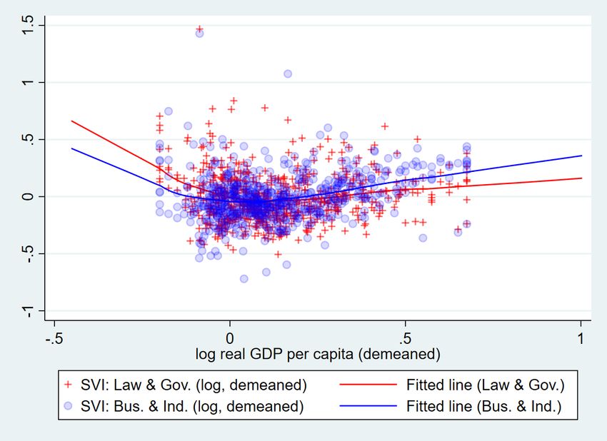
Some cases illustrate underlying relationships between SVIs and economic activities. For example, the
SVI for Myanmar under the travel category seems to capture the increasing trend of tourist arrivals to
Myanmar since 2011 (Figure 2). From the beginning of 2011, Myanmar underwent a series of political
reforms (IMF, 2015b). The following sections investigate whether this conjecture could be generalized,
110 based on regression analyses.
3. Can Google’s SVIs improve nowcasting performance for LIDCs?
3.1. Nowcasting model
To examine potential of Google’s SVIs, we consider a simple nowcasting model using SVIs. We construct
a panel data set of SVIs (the yearly averages of monthly data) from 2004 to 2017 for 59 LIDCs, combined
115 with macroeconomic data taken from several databases (see Table B.3 for variable definitions and data
sources; Table B.4 for summary statistics; and Table B.5 for pairwise correlation coefficients for selected
variables). We postulate a simple linear regression as follows:
Yit = ρYi,t−1 + βSV Iit + γXi,t−1 + αi + Dt + εit , (1)
where Yit denotes a variable to predict (real GDP growth, real exports, travel arrivals, inflation, exchange
rates, private capital inflows, FDI inflows); SV Iit denotes a vector of SVIs under the selected five categories;
120 Xit denotes a vector of other control variables; αi and Dt are country fixed effects and time dummies, re-
spectively; and εit denotes the residuals. See Table B.3 for how each variable is constructed and transformed
(e.g., in natural logarithm or in percent change).
5Figure 2: SVI under the travel category and tourist arrivals in Myanmar
Sources: Google Trends, World Development Indicators (World Bank, 2018), and the authors’ calculations.
Note: The SVI data are taken from the Google Trends website (https://trends.google.com/trends/explore?cat=67&date=
all&q=%2Fm%2F04xn_). SVI: search volume index.
This specification is motivated by real-time assessment of the economy when only lagged data are avail-
able. We put control variables Xit with a one-year lag, whereas the SVIs are contemporaneous, because our
125 purpose is to explore the benefits from timely observation of SVIs in real-time monitoring of the economy
where timely availability of macroeconomic statistics is an issue.5 For example, we consider a situation
to assess real GDP growth for the year 2016 as of January 2017 when actual real GDP and other related
macroeconomic data for 2016 were not yet available, although SVIs for 2016 were available. Control vari-
ables Xit are chosen based on the empirical literature on variables to nowcast (e.g., for economic growth
130 regression, Barro, 2015; for the determinants of capital flows, Araujo et al., 2017; Hashimoto and Wacker,
2016; Choi and Hashimoto, 2018), although many of the control variables that are used in the literature are
not included due to lack of observations for many LIDCs. For example, including the gross enrollment ratio
to secondary education reduces the sample size by one-third, while the results do not change significantly.
The purpose of the exercise is to find useful correlation between SVIs and economic variables, instead
135 of establishing causality. We aim to predict Yit by modeling the expected value of Yit conditional on all
the information available in a reduced form, instead of estimating structural causation between variables of
interest. See Kleinberg et al., 2015 for a useful distinction between prediction and causation.
High correlation across SVIs by category—ranging from 0.77 to 0.92 (Table A.5)—would not be a matter
of concern in predicting Yit .6 This is because the expected value of Yit conditional on highly collinear
140 variables should be similar to the one conditional on only one of the collinear variables, because highly
collinear variables should carry very similar amounts of information about Yit .7 Since the number of SVIs
that we use is five (or ten in extensions), there is little concern on a spurious perfect fit due to the large
number of regressors. However, such high correlation would pose a challenge in separating the category SVIs
into those that capture positive sentiments and those that capture negative sentiments.
145 Our model specification suffers from endogeneity issues. The issues stem from two-way causality between
Yit and SV Iit and from the inclusion of country fixed effects together with the lagged dependent variable
5 Our purpose is not backcasting, which aims to assess real-time measurement errors based on ex post information. Although
we use ex post data of SVIs, we consider this exercise as nowcasting, because the focus is still real-time economic monitoring.
6 Within correlation (i.e., correlation among SVIs demeaned by country) is somewhat lower (0.40-0.80, in most cases).
7 More generally, see Goldberger (1991, Chapter 23.3), echoed by (Hansen, 2019), for an argument that the issue of multi-
collinearity may be overemphasized.
6(the so-called Nickell bias problem; e.g., see Barro, 2015). In general, endogeneity issues do affect the
performance of prediction. For example, in the standard demand-supply estimation, an increase in quantity
by itself is only a mixed signal on the price. The price would increase or decrease, depending on whether
150 the quantity increase is driven by stronger demand or supply. The problem is, however, arguably much less
severe in the case where two-way causality shares the same direction, i.e., an increase in one variable always
implies an increase (or always implies a decrease) in the other variable, keeping other things constant. We
argue that the relationships between SVIs and economic variables of our interest fall in this case. After
all, how severe the endogeneity problem is can be assessed by the performance of prediction, although the
155 estimated coefficients would be anyway biased.
3.2. In-sample regression results
We find some of the SVIs show significance in the simple nowcasting model, contributing to a better fit
of the model. We confirm that these findings are robust to the issue of sampling, conducted in constructing
SVIs (see Appendix A for details), by repeating the same exercise for five separate vintages of the SVIs
160 constructed during April-June 2018. For ease of exposition, we refer to the SVI under a category in a
concise way; for example, the SVI under the business-and-industrial category is referred to the business-
industrial SVI, and so on. The findings are broadly similar when we do not include lagged covariates. While
interpreting the estimated coefficients needs some caution because of the estimation issues mentioned in the
previous section (i.e., endogeneity issues and the issue of multicollinearity among the SVIs), specific findings
165 are as follows:
• Economic activities (Table 2). The business-industrial SVI exhibits a significant positive correlation
with real GDP, indicating that a 10 percent increase in business-related attention would be associated
with a 0.7 percent increase in real GDP. The law -government SVI and the health SVI, on the other
hand, show significant negative correlations, implying that these SVIs may capture slowdowns in
170 economic activities due to public concerns on legal, political, or health issues. These SVIs show a
broadly similar pattern of correlation with real exports and tourist arrivals—with larger magnitudes—
, in line with a conjecture that people’s attention from outside of the country is the source of the
observed correlations. The travel SVI is positively correlated with tourist arrivals. We also try tourism
receipts, but the correlation is not as robust as for tourist arrivals, possibly because the SVI is more
175 associated with the number of people interested in visiting the country, rather than how much they
spend in the country.
• Prices (Table 3). There is strong positive correlation between inflation and the finance SVI—a 10
percent increase in finance-related attention would be associated with an increase in inflation by
0.3 percentage points. The results for the nominal exchange rate imply that the finance SVI may
180 reflect currency depreciation pressures and that its pass-through to inflation may explain the results
for inflation. Correlation between the finance SVI and the real effective exchange rate (REER) is
not significant, possibly due to relatively high pass-through in LIDCs. The law-government SVI
seems to be correlated with REER appreciation, which we admit is not so intuitive because the law-
government SVI is negatively associated with economic activities (as is shown in Table 2). The travel
185 SVI is significantly associated with lower prices, which would be due to people’s travel interests to a
destination with cheaper goods and services.
• Capital flows (Table 4). We find positive associations between gross capital inflows and the business-
industrial SVI. Motivated by Araujo et al. (2017), we separately examine FDI and non-FDI flows and
find somewhat stronger correlation for non-FDI flows. The finance SVI show no significant associ-
190 ation, possibly because the SVI may be more associated with individuals’ behaviors (e.g., checking
the exchange rate) and personal investment to these countries is not yet significant. The behaviors
of institutional investors may be better captured by the business-industrial SVI. The travel SVI is
negatively correlated with capital flows, which may reflect lower financing needs due to higher travel
service receipts.
7195 The findings are broadly robust to model uncertainty (Table 5). We employ the Bayesian model averaging
(BMA) methodology to examine robustness of our findings to specification uncertainty (Leamer, 1978). The
estimation is implemented using Stata command bma (De Luca and Magnus, 2011). The results show
that our findings are mostly robust to specification uncertainty, although the correlations with inflation and
capital flows are not so strong as they appear in Tables 3 and 4.
200 3.3. Comparison with nighttime lights
Nighttime lights (NLs) extracted from processed satellite imagery can also serve as a nontraditional source
of information for real-time economic monitoring, like SVIs. Since the seminal application by Henderson
et al. (2012), NLs have gained popularity as a proxy to the degree of economic activity (for a recent survey
on the economic applications of satellite data, see Donaldson and Storeygard, 2016). While Henderson et al.
205 (2012) compile annual data based on the Defense Meteorological Satellite Program Operational Linescan
System (DMSP OLS) data, a newer data set based on the Visible Infrared Imaging Radiometer Suite
(VIIRS) Day/Night Band (DNB) is available monthly since April 2012 (until October 2018 as of November
18, 2018), although its annual data set—with additional data cleaning—is available only for 2015 and 2016.8
We use the annual data compiled by the R package Rnightlights, developed by Njuguna (2018), while
210 cross-checking them with the data compiled by Henderson et al. (2012). The correlation between the two
NL data are almost one (Table B.5).
We benchmark SVIs with NLs and find that SVIs may contain stronger signals on economic activity
than NLs in LIDCs, while we find the opposite for EMEs. The significance of SVIs broadly remains while
NLs are not statistically significant for LIDCs (Table 6, columns 1-4). For EMEs, however, the opposite is
215 found—NLs are significant in the case of the OLS while SVIs are not (Table 6, columns 5-6). The weaker
performance of NLs for lower income countries is in line with the finding in the literature that the association
between NLs and output tends to be weaker for lower output areas (Chen and Nordhaus, 2011, Fig. 2, p.
8590). Further investigation indicates that the significance of NLs is lost for LIDCs when regressors include
the lag of covariates (Table B.6), whereas it is not lost for EMEs (Table B.7). The contrasting results imply
220 that there are some interesting structural differences between LIDCs and EMEs. For example, SVIs may
better capture external factors, which may be relatively more important in LIDCs, whereas NLs may better
reflect the level of domestic economic activity, which may play a larger role in EMEs than in LIDCs. The
comparison between LIDCs and EMEs is also discussed in Section 4.4.
The weak linkages between NLs and real GDP in LIDCs may need to be revisited to reflect methodological
225 refinements proposed in the literature. For example, Zhang et al. (2016) point out an issue of inconsistencies
in the temporal signal and propose a refined method to generate a globally consistent time series of NLs
from the DMSP OLS data. Their method leads to higher correlations between NLs and GDP than those
based on the standard method (Elvidge et al., 2009; Elvidge et al., 2014). Also, Hu and Yao (2019) uses
a nonparametric estimation framework to find important nonlinearity in the relationship between NLs and
230 real GDP. Debbich (2019) combines NLs and the data on radiant heat from gas flaring to strengthen the
estimated relationship between NLs and real GDP for oil-producing countries such as Yemen.
3.4. Out-of-sample nowcasting
We also examine out-of-sample performance of nowcasting. We conduct recursive nowcasting using 2012
as the starting year and calculate the mean squared error (MSE) of prediction for 2013-2016.9 Namely, we
235 predict the value of the variable of interest for 2013 by feeding observations available in 2013 (i.e., SVIs
for 2013 and other variables for 2012) using the model estimated by the observations up to 2012. We then
repeat this to predict values for 2014, 2015, and 2016, incrementally using more data to estimate the model.
8 See https://ngdc.noaa.gov/eog/viirs/download_dnb_composites.html. Both original NL data sources are compiled by
the initiatives under the National Oceanic and Atmospheric Administration (see the note under Table 6).
9 As our nowcasting models include country fixed effects and time dummies, we follow Calhoun (2014) to set the prediction
√
period to be close to the square root of the entire sample period (4 ' 13). The results may depend on the choice of the
starting year in general (Rossi and Inoue, 2012).
8Table 2: Economic activities and the search volume index (SVI) in LIDCs
(1) (2) (3) (4) (5) (6)
Dependent variables Real GDP Real exports Tourist arrivals
SVI: Finance 0.00 -0.00 0.01
(0.01) (0.04) (0.08)
SVI: Business and industrial 0.07*** 0.16* 0.25
(0.02) (0.09) (0.19)
SVI: Law and government -0.07*** -0.20*** -0.36***
(0.02) (0.07) (0.11)
SVI: Health -0.03** -0.02 -0.23**
(0.02) (0.03) (0.11)
SVI: Travel 0.00 0.02 0.23**
(0.01) (0.05) (0.09)
Lagged dependent variable 0.85*** 0.84*** 0.83*** 0.83*** 0.68*** 0.65***
(0.05) (0.05) (0.05) (0.05) (0.06) (0.06)
Population (lag) -0.03 -0.01 0.15 0.29 -1.12* -0.65
(0.13) (0.12) (0.41) (0.44) (0.56) (0.47)
Internet users (lag) -0.00 -0.00 0.02 0.02 0.02 0.04
(0.01) (0.00) (0.02) (0.02) (0.03) (0.03)
Real GDP (lag) -0.28* -0.31* -0.37 -0.48**
(0.15) (0.16) (0.25) (0.23)
Trade openness (lag) 0.02 0.01 -0.02 -0.05 -0.24** -0.29***
(0.01) (0.01) (0.09) (0.08) (0.11) (0.10)
Fiscal spending (lag) 0.04*** 0.03*** 0.06 0.04 0.24*** 0.22***
(0.01) (0.01) (0.05) (0.05) (0.07) (0.06)
REER, log level (lag) -0.03 -0.03 0.10 0.09 -0.36*** -0.36***
(0.03) (0.03) (0.09) (0.09) (0.13) (0.11)
Inflation (lag) -0.00* -0.00* -0.00 -0.00 -0.00 -0.00
(0.00) (0.00) (0.00) (0.00) (0.00) (0.00)
Trading partners’ growth (lag) 0.00 -0.00 -0.00 -0.00 0.03** 0.03**
(0.00) (0.00) (0.01) (0.01) (0.01) (0.01)
Export price growth (lag) 0.00 0.00 0.00 0.00 -0.00 -0.00
(0.00) (0.00) (0.00) (0.00) (0.00) (0.00)
Capital account openness (lag) 0.01 -0.01 0.14 0.09 0.30*** 0.18
(0.02) (0.02) (0.09) (0.09) (0.10) (0.12)
Age dependency ratio (lag) 0.00 -0.00 0.00 0.00 0.01 0.01
(0.00) (0.00) (0.01) (0.00) (0.01) (0.01)
Observations 644 644 633 633 575 575
Number of countries 53 53 53 53 52 52
Adjusted R-squared 0.961 0.964 0.797 0.802 0.743 0.763
Country fixed effects YES YES YES YES YES YES
Time dummies YES YES YES YES YES YES
Sources: Chinn and Ito (2006), Google Trends, International Financial Statistics (IMF, 2018b),
World Development Indicators (World Bank, 2018), World Economic Outlook (IMF, 2018e), and
the authors’ estimation.
Note. Sample period: 2004-2016. Cluster-robust standard errors are reported in parentheses.
Superscripts *, **, and *** indicate statistical significance at the 10 percent, 5 percent, and 1
percent level, respectively. See Table B.1 for country groupings and Table B.3 for variable definitions
(most of variables are in natural logarithm or percent change) and data sources. LIDCs: low-income
developing countries; REER: real effective exchange rate; SVI: search volume index.
9Table 3: Price developments and the search volume index (SVI) in LIDCs
(1) (2) (3) (4) (5) (6)
Nominal exchange rate
Inflation REER
Dependent variables (local currencies to one U.S.
(percent change) (percent change)
dollar, percent change)
SVI: Finance 3.36*** 7.83*** -2.49
(1.04) (2.32) (1.68)
SVI: Business and industrial -2.93* -0.57 -0.90
(1.47) (3.48) (2.73)
SVI: Law and government 0.48 -5.72** 4.68**
(1.20) (2.22) (2.21)
SVI: Health 1.53 0.05 0.19
(0.99) (1.58) (1.38)
SVI: Travel -2.90** -2.99 0.69
(1.25) (2.52) (1.89)
Lagged dependent variable 0.34*** 0.32*** 0.13*** 0.11*** 0.04 0.04
(0.05) (0.05) (0.03) (0.03) (0.03) (0.04)
Population (lag) 0.25 0.09 -6.19 1.65 14.24 10.67
(14.79) (15.96) (16.98) (18.78) (9.45) (11.28)
Internet users (lag) 0.96** 0.82* 0.82 0.52 -0.36 -0.39
(0.42) (0.43) (0.81) (0.79) (0.69) (0.67)
Real GDP (lag) 0.75 1.49 2.59 3.40 -1.43 -1.43
(3.15) (3.16) (4.77) (5.00) (5.81) (5.45)
Trade openness (lag) -0.10 0.45 -6.89*** -6.37** 7.23*** 7.55***
(1.08) (1.08) (2.27) (2.45) (2.03) (2.22)
Fiscal spending (lag) -1.58 -1.83 -3.62* -5.04** 2.22 2.90
(1.12) (1.14) (1.90) (1.95) (2.19) (2.16)
REER, percent change (lag) -0.20*** -0.20***
(0.03) (0.03)
Inflation (lag) -0.09** -0.10** 0.24** 0.25**
(0.04) (0.04) (0.11) (0.12)
Trading partners’ growth (lag) -0.07 -0.06 -0.36 -0.35 -0.51 -0.52
(0.21) (0.20) (0.32) (0.31) (0.33) (0.34)
Import price growth (lag) 0.06 0.08 -0.11 -0.12 0.17 0.20*
(0.06) (0.06) (0.09) (0.10) (0.11) (0.11)
Capital account openness (lag) -2.98 -1.84 -4.69 -4.57 0.45 1.06
(3.10) (2.70) (4.15) (3.52) (3.15) (3.06)
Age dependency ratio (lag) -0.02 -0.02 0.31* 0.30* -0.29*** -0.27**
(0.13) (0.13) (0.17) (0.17) (0.10) (0.10)
Observations 642 642 671 671 641 641
Number of countries 54 54 55 55 54 54
Adjusted R-squared 0.306 0.319 0.304 0.326 0.153 0.158
Country fixed effects YES YES YES YES YES YES
Time dummies YES YES YES YES YES YES
Sources: Chinn and Ito (2006), Google Trends, International Financial Statistics (IMF, 2018b), World Devel-
opment Indicators (World Bank, 2018), World Economic Outlook (IMF, 2018e), and the authors’ estimation.
Note. Sample period: 2004-2016. Cluster-robust standard errors are reported in parentheses. Superscripts
*, **, and *** indicate statistical significance at the 10 percent, 5 percent, and 1 percent level, respectively.
See Table B.1 for country groupings and Table B.3 for variable definitions (most of variables are in natural
logarithm or percent change) and data sources. LIDCs: low-income developing countries; REER: real
effective exchange rate; SVI: search volume index.
10Table 4: Capital flows and the search volume index (SVI) in LIDCs
(1) (2) (3) (4) (5) (6) (7) (8)
Total capital Private capital
Dependent variables FDI inflows Non-FDI inflows
inflows inflows
SVI: Finance -0.23 -0.17 -0.12 -0.32
(0.23) (0.20) (0.27) (0.29)
SVI: Business and industrial 1.19*** 0.94*** 1.24** 1.49***
(0.30) (0.35) (0.53) (0.50)
SVI: Law and government -0.22 0.06 -0.32 -0.05
(0.32) (0.26) (0.32) (0.29)
SVI: Health -0.47** -0.36 -0.39* -0.19
(0.21) (0.25) (0.22) (0.21)
SVI: Travel -0.28 -0.58*** -0.21 -0.64**
(0.18) (0.19) (0.24) (0.28)
Lagged dependent variable 0.16** 0.14* 0.08 0.06 0.23*** 0.21*** 0.07 0.02
(0.08) (0.08) (0.10) (0.09) (0.06) (0.06) (0.08) (0.08)
Population (lag) 0.01 -1.00 -0.62 -2.22* 0.22 -0.01 0.78 -0.45
(1.34) (1.39) (1.30) (1.19) (1.23) (1.30) (1.52) (1.62)
Internet users (lag) 0.15* 0.10 0.19* 0.15 0.13 0.09 0.15 0.06
(0.08) (0.09) (0.10) (0.10) (0.13) (0.13) (0.14) (0.13)
Real GDP (lag) 0.47 0.56 1.04* 1.14* 0.96 0.94 -0.06 0.18
(0.63) (0.62) (0.61) (0.59) (0.90) (0.86) (0.93) (0.97)
Trade openness (lag) 0.55* 0.51* 0.68** 0.67** 0.55* 0.53* 1.27*** 1.33***
(0.29) (0.26) (0.29) (0.26) (0.29) (0.30) (0.40) (0.36)
Fiscal spending (lag) 0.26 0.26 0.30 0.33 0.11 0.07 -0.25 -0.31
(0.24) (0.26) (0.23) (0.22) (0.26) (0.27) (0.35) (0.37)
REER, log level (lag) -0.15 -0.14 -0.13 -0.12 -0.05 0.06 0.04 0.16
(0.40) (0.36) (0.41) (0.38) (0.39) (0.36) (0.69) (0.68)
Inflation (lag) -0.01 -0.01 -0.01 -0.01 -0.01 -0.01 -0.01 -0.01
(0.01) (0.01) (0.01) (0.01) (0.01) (0.01) (0.01) (0.01)
Trading partners’ growth (lag) 0.05 0.05 0.05 0.05 0.04 0.04 -0.00 0.00
(0.04) (0.04) (0.04) (0.04) (0.03) (0.03) (0.04) (0.04)
Export price growth (lag) 0.01 0.01 -0.01 -0.00 0.01 0.01 -0.03** -0.02
(0.02) (0.02) (0.02) (0.01) (0.01) (0.01) (0.02) (0.02)
Capital account openness (lag) 0.11 0.02 0.45 0.55 -0.39 -0.54 1.73*** 1.93***
(0.52) (0.59) (0.42) (0.44) (0.45) (0.44) (0.48) (0.45)
Age dependency ratio (lag) 0.00 0.01 0.00 0.00 -0.02 -0.02 -0.03 -0.03
(0.02) (0.02) (0.02) (0.02) (0.02) (0.02) (0.03) (0.03)
Observations 461 461 454 454 535 535 377 377
Number of countries 49 49 49 49 49 49 48 48
Adjusted R-squared 0.424 0.437 0.419 0.433 0.339 0.348 0.390 0.414
Country fixed effects YES YES YES YES YES YES YES YES
Time dummies YES YES YES YES YES YES YES YES
Sources: Chinn and Ito (2006), Financial Flows Analytics (IMF, 2018a), Google Trends, International Financial
Statistics (IMF, 2018b), World Development Indicators (World Bank, 2018), World Economic Outlook (IMF,
2018e), and the authors’ estimation.
Note. Sample period: 2004-2016. Cluster-robust standard errors are reported in parentheses. Superscripts *, **,
and *** indicate statistical significance at the 10 percent, 5 percent, and 1 percent level, respectively. See Table B.1
for country groupings and Table B.3 for variable definitions (most of variables are in natural logarithm or percent
change) and data sources. LIDCs: low-income developing countries; REER: real effective exchange rate; SVI: search
volume index.
11Table 5: Bayesian model averaging results for LIDCs
(1) (2) (3) (4) (5) (6) (7)
Nominal Private
Real Real Tourist FDI
Dependent variables Inflation exchange capital
GDP exports arrivals inflows
rate inflows
SVI: Finance 0.00 0.00 0.01 1.72 6.20 0.00 0.01
[0.04] [0.06] [0.09] [0.67] [0.96] [0.06] [0.07]
SVI: Business and industrial 0.07 0.11 0.19 -0.12 -0.39 0.40 0.36
[1.00] [0.76] [0.65] [0.08] [0.10] [0.56] [0.52]
SVI: Law and government -0.07 -0.17 -0.34 0.04 -3.89 -0.00 -0.05
[1.00] [0.97] [1.00] [0.05] [0.68] [0.06] [0.12]
SVI: Health -0.03 0.00 -0.19 0.05 -0.14 -0.16 -0.08
[0.94] [0.05] [0.81] [0.06] [0.07] [0.33] [0.20]
SVI: Travel -0.00 0.00 0.24 -1.49 -1.63 -0.14 -0.01
[0.04] [0.06] [0.97] [0.53] [0.38] [0.32] [0.06]
Lagged dependent variable 0.83 0.81 0.65 0.34 0.10 0.03 0.26
[1.00] [1.00] [1.00] [1.00] [0.83] [0.27] [1.00]
Population (lag) 0.00 0.01 -0.05 -0.03 0.31 -0.04 0.01
[0.04] [0.06] [0.10] [0.04] [0.05] [0.06] [0.04]
Internet users (lag) -0.00 0.00 0.00 0.24 0.03 0.11 0.05
[0.04] [0.08] [0.08] [0.30] [0.05] [0.55] [0.30]
Real GDP (lag) -0.07 -0.21 -0.01 0.07 1.38 0.56
[0.38] [0.53] [0.04] [0.05] [0.80] [0.41]
Trade openness (lag) 0.00 -0.00 -0.23 -0.00 -7.12 0.76 0.21
[0.10] [0.05] [0.90] [0.04] [0.98] [0.95] [0.37]
Fiscal spending (lag) 0.03 0.00 0.16 -0.17 -2.66 0.13 0.03
[0.98] [0.05] [0.82] [0.13] [0.70] [0.33] [0.11]
REER, log level (lag) -0.00 0.02 -0.30 -0.00 0.00
[0.11] [0.15] [0.88] [0.05] [0.04]
REER, percent change (lag) -0.19
[1.00]
Inflation (lag) -0.00 -0.00 -0.00 -0.05 -0.00 -0.00
[0.09] [0.06] [0.04] [0.53] [0.08] [0.05]
Trading partners’ growth (lag) 0.00 -0.00 0.01 -0.00 -0.02 0.01 0.00
[0.05] [0.06] [0.24] [0.04] [0.07] [0.11] [0.09]
Export price growth (lag) -0.00 0.00 -0.00 -0.00 0.00
[0.36] [0.07] [0.04] [0.05] [0.07]
Import price growth (lag) 0.01 -0.02
[0.08] [0.11]
Capital account openness (lag) -0.00 0.01 0.01 -0.18 -0.44 0.04 -0.02
[0.04] [0.09] [0.06] [0.07] [0.09] [0.09] [0.05]
Age dependency ratio (lag) -0.00 0.00 0.00 - 0.00 0.25 -0.00 -0.00
[0.04] [0.05] [0.08] [0.04] [0.70] [0.05] [0.07]
Observations 644 633 575 642 671 454 535
Number of countries 54 54 53 54 55 49 49
Country fixed effects YES YES YES YES YES YES YES
Time dummies YES YES YES YES YES YES YES
Sources: Chinn and Ito (2006), Financial Flows Analytics (IMF, 2018a), Google Trends, International
Financial Statistics (IMF, 2018b), World Development Indicators (World Bank, 2018), World Economic
Outlook (IMF, 2018e), and the authors’ estimation.
Note. Sample period: 2004-2016. Posterior inclusion probability (PIP) are reported in brackets. The
coefficients are bolded if PIP exceeds 0.5, corresponding to what is known as the median probability
model (Barbieri and Berger, 2004). The estimation is implemented using Stata command bma (De Luca
and Magnus, 2011). See Table B.1 for country groupings and Table B.3 for variable definitions (most of
variables are in natural logarithm or percent change) and data sources. LIDCs: low-income developing
countries; REER: real effective exchange rate; SVI: search volume index.
12Table 6: Search volume index (SVI) and nighttime lights (NLs)
(1) (2) (3) (4) (5) (6)
Dependent variables Real GDP
LIDCs EMEs
OLS BMA OLS BMA OLS BMA
SVI: Finance 0.01 0.01 0.01 0.00 0.00 0.00
(0.02) [0.25] (0.01) [0.06] (0.01) [0.04]
SVI: Business and industrial 0.02 0.00 0.06*** 0.05 -0.01 -0.00
(0.03) [0.14] (0.02) [1.00] (0.01) [0.10]
SVI: Law and government -0.06*** -0.07 -0.08*** -0.08 -0.00 -0.00
(0.02) [0.99] (0.02) [1.00] (0.01) [0.06]
SVI: Health -0.01 0.00 -0.01 -0.00 -0.02 -0.01
(0.01) [0.06] (0.02) [0.07] (0.01) [0.19]
SVI: Travel 0.02 0.00 0.00 -0.00 0.01 0.00
(0.02) [0.19] (0.02) [0.05] (0.01) [0.05]
NLs from HSW (2012) 0.01 0.00
(0.02) [0.06]
NLs from HSW (2012) (lag) -0.01 -0.00
(0.01) [0.06]
NLs from Rnightlights 0.01 0.00 0.02** 0.00
(0.01) [0.08] (0.01) [0.11]
NLs from Rnightlights (lag) -0.01 -0.00 -0.02** -0.00
(0.01) [0.04] (0.01) [0.06]
Control variables included YES YES YES YES YES YES
Observations 241 241 545 545 711 711
2004-2013, 2004-2013, 2004-2013, 2004-2013,
Sample period 2004-2008 2004-2008
2015-2016 2015-2016 2015-2016 2015-2016
Number of countries 53 53 53 53 70 70
Adjusted R-squared 0.937 - 0.969 - 0.961 -
Country fixed effects YES YES YES YES YES YES
Time dummies YES YES YES YES YES YES
Excluding periods of jumps NO NO NO NO NO NO
Sources: Chinn and Ito (2006); Earth Observation Group; Financial Flows Analytics (IMF, 2018a); GADM
(2018); Google Trends; Henderson et al. (2012); International Financial Statistics (IMF, 2018b); National
Geophysical Data Center (with U.S. Air Force Weather Agency); World Development Indicators (World Bank,
2018); World Economic Outlook (IMF, 2018e); and the authors’ estimation.
Note. For ordinary least squares (OLS), cluster-robust standard errors are reported in parentheses. Superscripts
*, **, and *** indicate statistical significance at the 10 percent, 5 percent, and 1 percent level, respectively.
For Bayesian model averaging (BMA), posterior inclusion probability (PIP) are reported in brackets. The
coefficients are bolded if PIP exceeds 0.5, corresponding to what is known as the median probability model
(Barbieri and Berger, 2004). The estimation is implemented using Stata command bma (De Luca and Magnus,
2011). The NLs from HSW (2012) line shows the coefficients on NL data (variable lndn) compiled by Henderson
et al. (2012), available for 1992-2008. The NLs from Rnightlights line shows the coefficients on NL data
compiled by R package Rnightlights developed by Njuguna (2018), available for 1992-2013 based on DMSP
OLS data (also used by Henderson et al., 2012) and for 2015-2016 based on the Visible Infrared Imaging
Radiometer Suite (VIIRS) Day/Night Band (DNB) data. The DMSP OLS data are based on the processed
images provided by National Geophysical Data Center, while images are collected by U.S. Air Force Weather
Agency. The VIIRS DNB data are produced by the Earth Observation Group, NOAA/NCEI. See Table B.1
for country groupings and Table B.3 for variable definitions (most of variables are in natural logarithm or
percent change) and data sources. Among EMEs, the NL data exclude countries identified as outliers by
Henderson et al. (2012, footnote 16, p. 1011; Bahrain, Equatorial Guinea, Serbia, Montenegro). For the data
compiled by Rnightlights, several large economies are also excluded due to their heavy computational burden
(Brazil, Chile, China, Indonesia, India, Mexico, Peru, Russia). DMSP OLS: Defense Meteorological Satellite
Program Operational Linescan System; EMEs: emerging market economies; LIDCs: low-income developing
countries; NCEI: National Centers for Environmental Information; NOAA: National Oceanic and Atmospheric
Administration; REER: real effective exchange rate; SVI: search volume index.
13We compare the best predicting models selected from the pool of variables with and without SVIs. As
including irrelevant variables to a model may increase the MSE, we conduct an exhaustive search from the
240 pool of SVIs and control variables to identify the set of variables with which the linear regression model
minimizes the MSE, combined with country fixed effects and time dummies. We then do this again only for
control variables, without SVIs, and compare the MSEs between the two best predicting models.10
This way, we find that adding SVIs to the pool of variables improves performance in nowcasting economic
indicators. We find that for all economic indicators to predict, the MSE of the best model is lower when
245 including SVIs in the pool of selection, in the case of LIDCs (Table 7, Panel A). The differences in MSEs
between the best models with and without SVIs are not very large in general nor statistically significant.
Note, however, that most of our comparisons are between nested models and the standard statistical inference
based on the Diebold-Mariano test (Diebold and Mariano, 1995) across nested models may not be valid,
especially in the presence of autocorrelation or cross-panel dependency (e.g., see Diebold, 2015, for the review
250 of the literature). The SVIs included in the best model are generally in line with the in-sample analysis, but
not always the same. For example, for real GDP, while the law-government SVI is always selected in the top
10 models in terms of the MSE, as is significant in the in-sample results, the business-industrial SVI is not
selected, but instead, the finance SVI is selected (Table B.8). Further investigation would be interesting to
reconcile in-sample and out-of-sample results, as is discussed in the literature (e.g., Inoue and Kilian, 2005;
255 Diebold, 2015, and associated comment papers).
4. Extensions
4.1. Jumps in SVIs
We observe jumps (or positive outliers) in SVIs occasionally. These acute increases in the SVIs are
associated with critical events, including natural disasters, major policy changes, and key developments in
260 the business environment. We identify 178 jumps in the SVI for the “all” category (i.e., with no category
specified) out of 804 observations in our sample for LIDCs, using a methodology in the finance literature
(Lee and Mykland, 2008). The difference between the squared percent change and the consecutive absolute
percent change (called bi-power variations) indicates a huge change in the SVI within a period (see Appendix
A.5 for details). The reason for not using each SVI by category for the jump detection is to focus on very
265 acute increases in individuals’ attention that are significant enough to stand out in the SVI with no category
specified, even though their causes would be category-specific.
Excluding the periods when a jump occurred seems to sharpen estimation results. As each jump would
have a very different implication from one another, we exclude those periods with jumps from the sample
and re-estimate our models. The results show more statistical significance in many cases, while there is no
270 significant change for inflation and the significance rather weakens for real exports and FDI inflows (Table
B.10). This implies that jumps in SVIs could indicate the periods when their relationships with economic
variables become unstable or strongly nonlinear, and that excluding such periods either strengthens the true
linear relationships or weakens the spurious significance.
4.2. Lagged effects
275 There could be time lags for people’s attentions to materialize as actual economic actions. Search of
background information would happen before travel or investment take place. In this regard, SVIs could
rather serve as a leading indicator.
In our specifications, lagged SVIs do not show significant correlation as clearly as contemporaneous SVIs
do (Table B.11). This is probably because our models are at the annual frequency and the one-year lag
280 could be too long. An exception is the case of private capital flows where lagged SVIs work better. For
real GDP, lagged SVIs seem to complement contemporaneous SVIs. More meaningful leading signals could
possibly be found in the SVIs at a higher frequency such as monthly, although limited availability of other
indicators at a higher frequency would pose a challenge for such an analysis.
10 We also compare the averages of the lowest 10 MSEs, instead of only the lowest MSE, and find very similar results.
14Table 7: Out-of-sample performance of nowcasting
Nominal Private
Real Real Tourist FDI
Inflation exchange capital
GDP exports arrivals inflows
rate inflows
Panel A. MSE of the best model with fixed and time effects — LIDCs
Controls only 0.37 1.60 7.58 0.12 0.83 60.84 122.40
Controls + SVIs 0.36 1.59 6.89 0.11 0.73 55.96 117.68
Difference (in percent) -2.6 -1.0 -10.0 -7.4 -14.4*** -8.7*** -4.0
Panel B. MSE of the best model with fixed and time effects — EMEs
Controls only 0.09 0.77 1.92 0.45 1.00 75.45 47.90
Controls + SVIs 0.08 0.76 1.92 0.44 0.95 75.22 47.90
Difference (in percent) -3.1 -1.4 0.0 -2.0 -5.5*** -0.3 0.0
Sources: Chinn and Ito (2006), Financial Flows Analytics (IMF, 2018a), Google Trends, International
Financial Statistics (IMF, 2018b), World Development Indicators (World Bank, 2018), World Economic
Outlook (IMF, 2018e), and the authors’ estimation.
Note. We conduct recursive nowcasting using a panel data set from 2004 to 2016. We set 2012 as the starting
year and calculate the mean squared error (MSE) of prediction for 2013-2016. We predict the value of the
variable of interest for 2013, by feeding observations available in 2013 (i.e., SVIs for 2013 and other controls
for 2012) using the model estimated by the observations up to 2012. We then repeat this to predict values for
2014, 2015, and 2016, incrementally using more data to estimate the model. We include country fixed effects
and time dummies, from which we back out the averaged constant term so that country fixed effects and time
effects are redefined as deviations from the constant term, and thus, ex ante time effects for prediction years
can be assumed to be zero. Panel A shows the results for LIDCs and Panel B shows the results for EMEs.
The Control variables + SVIs lines show the minimum MSEs identified by an exhaustive search from the
pool of all variables to be included in the model. The Controls only lines show the minimum MSEs identified
by an exhaustive search from the pool of control variables, excluding the SVIs. See Tables B.8 and B.9 for
the best model specifications chosen in this procedure. To overcome a computational challenge stemming
from the exhaustive search across variables to include, we follow the algorithm proposed by Somaini and
Wolak (2016) to speed up the calculation to estimate regressions with two-way fixed effects. The Difference
(in percent) lines show the differences of the above two lines in percent of the second line. Superscripts *, **,
and *** indicate statistical significance at the 10 percent, 5 percent, and 1 percent level, respectively, based
on a Diebold-Mariano test (Diebold and Mariano, 1995) using cluster-robust standard errors, although it
should be noted that most of these model comparisons are between nested models and conducting statistical
inference across nested models is not trivial, especially when forecasting errors could exhibit autocorrelation
or cross-panel dependency (e.g., see Diebold, 2015, for a review of the literature). The nominal exchange
rate is the local currency per U.S. dollar, transformed to annual percent changes, period average. See Table
B.1 for country groupings and Table B.3 for variable definitions (most of variables are in natural logarithm
or percent change) and data sources. For inflation and nominal exchange rate, we divide them by 100 to be
comparable to other logged variables for this table. EMEs: emerging market economies; LIDCs: low-income
developing countries; SVI: search volume index.
154.3. Searches made domestically
285 We further examine SVIs on the searches made domestically. We construct an additional data set of
SVIs by changing the location from “worldwide” to each country of interest—e.g., searches about Bangladesh
made in Bangladesh. We refer to these SVIs as domestic SVIs. The domestic SVIs would capture individuals’
attention to a country in that country. The domestic SVIs are more likely to be subject to the issue of low
responses and the reporting cut-off, but they would potentially capture certain activities (especially those
290 that happened locally) better than the worldwide SVIs.
Including domestic SVIs do not generally change the regression results, implying that the major source
of information from worldwide SVIs is attention from foreign locations. Results do not change for most
of the cases, except capital flows, which now show weaker correlation (Appendix Table 12). The domestic
business-industrial SVI is negatively associated with inflation, which may reflect the importance of inflation
295 for local businesses.
4.4. Does it work for EMEs too?
We also investigate whether Google’s SVIs would be useful for macroeconomic analyses in EMEs. Our
work can naturally extend to EMEs, many of which share common characteristics with LIDCs (see Table
B.1 for the list of the EMEs and Table B.13 for summary statistics for EMEs).
300 For EMEs, the correlations between SVIs and macroeconomic variables are not as robust as those for
LIDCs (Table B.14). As discussed in Section 3.3, the weaker correlations might imply relatively weaker
influences of the external factors to EMEs than LIDCs—due to larger domestic markets in EMEs—because
SVIs may better capture external factors related to online searches from abroad. Another reason could
be that investors’ behaviors to gain information about EMEs through the Internet may not be significant
305 signals among other key factors in more matured and complicated financial markets in EMEs than those in
LIDCs. Similarly, adding SVIs does not improve the nowcasting accuracy for EMEs as much as it does for
LIDCs (Table 7, Panel B; Table B.9).
4.5. Machine learning algorithms
We apply some of machine learning algorithms, which are increasingly becoming popular in economic
310 analyses (Varian, 2014; Mullainathan and Spiess, 2017). As these algorithms are mainly used to produce out-
of-sample projections, we compare out-of-sample performances with our best linear models in Section 3.4.
We examine LASSO-type regressions (implemented using lassopack by Ahrens et al., 2018) and Random
Forest (implemented using the scikit-learn package in Python by Pedregosa et al., 2011).
The results are broadly similar to our findings in Section 3.4. LASSO-type regressions select a sim-
315 ilar set of SVIs in the final projection models. For these methods, out-of-sample MSEs are larger than
our best linear models, because their final projection models are still linear and our best linear models
achieve the minimum MSEs by construction. As for Random Forest (implemented using the module en-
semble.ExtraTreesRegressor of the scikit-learn package), we find slight improvements in MSEs compared
to our best linear models and the MSEs are slightly smaller for the models that include SVIs than those do
320 not. A more comprehensive analysis would potentially find further refinements of our results so far.
5. Conclusion
This paper presents an effort to use advanced technology to address the recurrent issue of lack of infor-
mation in policy-making and analysis for developing economies. While progress has been made in timely
provision of official data, nontraditional data obtained through recent technology have enormous potential
325 to fill information gaps in developing economies. We investigate how much information we could obtain from
Internet search frequencies to strengthen the capacity to monitor and assess current economic developments.
Our findings provide important steps forward in utilizing Google Trends’ data in economic analyses. The
in-sample and out-of-sample performances of a simple nowcasting model demonstrates the usefulness of the
information contained in Google’s SVI. The contrasting results between LIDCs and EMEs regarding the
330 comparison of SVIs and another new source of information—nighttime lights—not only demonstrate the
16You can also read